We discuss the phenomenology of $(1,1)$-mode adjoint scalars in the framework of two Universal Extra Dimensions. The Kaluza-Klein (KK) towers of these adjoint scalars arise in the 4-dimensional effective theory from the 6th component of the gauge fields after compactification. Adjoint scalars can have KK-number conserving as well as KK-number violating interactions. We calculate the KK-number violating operators involving these scalars and two Standard Model fields. Decay widths of these scalars into different channels have been estimated. We have also briefly discussed pair-production and single production of such scalars at the Large Hadron Collider.

1 Introduction

The primary aim for the next generation particle physics experiments will be to find out whether a new dynamics beyond the Standard Model (SM) really exists around the TeV scale of energy. A great effort have been put in also to pin down the exact nature of this new dynamics at the TeV Scale. In this endeavour, lots of attention have been paid to the theories with one or more extra space like dimensions. These extra dimensional theories can be classified into two main classes. In one of these, the standard model fields are confined to a (3 + 1) dimensional subspace of the full manifold. Models of ADD [1] or RS [2] fall in this category. On the other hand, there are class of models where some or all of the SM fields can access the full space-time manifold. One such example is Universal Extra Dimension (UED), where all the fields can propagate in the full manifold [3]. Apart from the rich phenomenology, UED models in general offer possible unification of the gauge couplings at a relatively low scale of energy, not far beyond the reach of the next generation colliders [4]. Moreover, particle spectra of UED models contain a weakly interacting stable massive particle, which can be a good candidate for cold dark matter [5, 6].

Phenomenology of one UED (1UED, space time is $4+1$ dimensional), have been extensively studied in the context of low energy experiments [7] as well as high energy collider experiments [8]. In this article, we will study some aspects of a particular variant of the UED model where all the SM fields can access 5 space like and 1 time like dimensions. This is called two Universal Extra Dimension (2UED) Model which has few additional attractive features. 2UED model can naturally explain the long life time for the proton decay [9] and more interestingly predicts that the number of fermion generations should be an integral multiple of three [10].

Recently, signals of 2UED model in future colliders like LHC [11, 12] and ILC [13] have been studied in some details. In this article, we will concentrate on the phenomenology of some of the scalars in this theory and their possible production at the LHC.

In $(1+5)$ dimensional (6D) space time, gauge fields have 6 components. However, after compactification, $(1+3)$ dimensional (4D) effective theory comprises of usual SM gauge fileds along with their Kaluza-Klein (KK) excitations. The 6th component of the gauge fields emerge as KK towers of scalar fields transforming as the adjoints of the respective gauge groups. Each KK-mode fields in 2UED model is specified by a pair of positive integers (called the KK-numbers). Phenomenology of the $(1,1)$-mode adjoint scalars will be discussed in this article.

The plan of the article is the following. We will give a brief description of the model in the next section. Interactions of the adjoint scalars will be discussed in section 3. Section 4 will be devoted to the decays of the $(1,1)$-mode adjoint scalars. We will briefly discuss the possible production mechanism of these scalars in section 5. We summarise in the last section.

2 Two Universal Extra Dimensions

As the name suggests, in 2UED all the SM fields can propagate universally in the six-dimensional space-time. Four space time coordinates $x^{\mu}$ ($\mu=0,1,2,3$) form the usual Minkowski space. Two transverse spacial dimensions of coordinates $x^{4}$ and $x^{5}$ are flat and are compactified with $0\leq~{}x^{4},~{}x^{5}~{}\leq L$. This implies that the extra dimensional space (before compactification) is a square with sides $L$. Identifying the opposite sides of the square will make the compactified manifold a torus. However, toroidal compactification, leads to 4D fermions that are vector-like with respect to any gauge symmetry. The alternative is to identify two pairs of adjacent sides of the square:

$$(y,0)~{}\equiv~{}(0,y),~{}~{}~{}(y,L)~{}\equiv~{}(L,y),~{}~{}~{}\forall~{}y\in~{}[0,L]$$ (1)

This is equivalent to folding the square along a diagonal and gluing the boundaries. Above compactification mechanism automatically leaves at most a single 4D fermion of definite chirality as the zero mode of any chiral 6D fermion [14].

The field values should be equal at the identified points, modulo possible other symmetries of the theory. The physics at identified points is identical if the Lagrangian takes the same value for any field configuration:

$${\cal L}|_{x^{\mu},y,0}\;=\;{\cal L}|_{x^{\mu},0,y};~{}~{}{\cal L}|_{x^{\mu},y,L}\,=\,{\cal L}|_{x^{\mu},L,y}$$

This requirement fixes the boundary conditions for 6D scalar fields $\Phi(x^{\alpha})$ and 6D Weyl fermions $\Psi_{\pm}(x^{\alpha})$. The requirement that the boundary conditions for 6D scalar or fermionic fields are compatible with the gauge symmetry, also fixes the boundary conditions for 6D gauge fields. The folding boundary conditions do not depend on continuous parameters, rather there are only eight self-consistent choices out of which one particular choice leads to zero mode fermions after compactification. Any 6D field (fermion/gauge or scalar) $\Phi(x^{\mu},x^{4},x^{5})$ can be decomposed as:

$$\Phi(x^{\mu},x^{4},x^{5})~{}=~{}\frac{1}{L}\sum_{j,k}f^{(j,k)}_{n}(x^{4},x^{5})\Phi^{(j,k)}(x^{\mu})$$ (2)

Where,

$$f^{(j,k)}_{n}(x^{4},x^{5})~{}=~{}\frac{1}{1~{}+~{}\delta_{j,0}\delta_{k,0}}\left[e^{-in\pi/2}cos\left(\frac{jx^{4}+kx^{5}}{R}~{}+~{}\frac{n\pi}{2}\right)~{}+~{}cos\left(\frac{kx^{4}-jx^{5}}{R}~{}+~{}\frac{n\pi}{2}\right)\right]$$ (3)

The compactification radius $R$ is related to the size, $L$, of the compactified space as : $L=\pi R$. Where 4D fields $\Phi^{(j,k)}(x^{\mu})$ are the $(j,k)$-th KK modes of the 6D field $\Phi(x^{\alpha})$ and $n$ is a integer whose value is restricted to $0,1,2$ or $3$ by the boundary conditions. It is obvious from the form of $f^{(j,k)}_{n}(x^{4},x^{5})$ that only $n=0$ allows zero mode ($j=k=0$) fields in the 4D effective theory. The zero mode fields and the interactions among zero modes can be identified with the SM.

The requirements of anomaly cancellation and fermion mass generation force the weak-doublet fermions to have opposite 6D chiralities with respect to the weak-singlet fermions. So the quarks of one generation are given by $Q_{+}~{}\equiv~{}(U_{+},D_{+}),~{}U_{-},~{}D_{-}$. The 6D doublet quarks and leptons decompose into a tower of heavy vector-like 4D fermion doublets with left-handed zero mode doublets. Similarly each 6D singlet quark and lepton decompose into the towers of heavy 4D vector-like singlet fermions along with zero mode right-handed singlets. These zero mode fields are identified with the SM fermions. As for example, SM doublet and singlets of 1st generation quarks are given by $(u_{L},d_{L})~{}\equiv~{}Q_{+L}^{(0,0)}(x^{\mu})$, $u_{R}~{}\equiv~{}U_{-R}^{(0,0)}(x^{\mu})$ and $d_{R}~{}\equiv~{}D_{-R}^{(0,0)}(x^{\mu})$.

In 6D, each of the gauge fields, has six components. Upon compactification, they decompose into towers of 4D spin-1 fields, a tower of spin-0 fields which are eaten by heavy spin-1 fields. Another tower of 4D spin-0 fields, all belonging to the adjoint representation of the corresponding gauge group, remain in the physical spectrum. These are the physical spinless adjoints in which we are interested.

The tree-level masses for $(j,k)$-th KK-mode particles are given by $\sqrt{M_{j,k}^{2}~{}+~{}m_{0}^{2}}$, where $M_{j,k}=\sqrt{j^{2}+k^{2}}/R$. $m_{0}$ is the mass of the corresponding zero mode particle. As a result, the tree-level masses are approximately degenerate. This degeneracy is lifted by radiative effects. The fermions receive mass corrections from the gauge interactions (with gauge bosons and adjoint scalars) and Yukawa interactions. All of these give positive mass shift. The gauge fields and spinless adjoints receive mass corrections from the self-interactions and gauge interactions. Gauge interactions with fermions give a negative mass shift. While the self-interactions give positive mass shift with different strength with respect to the former. However, masses of the hypercharge gauge boson $B_{\mu}^{(j,k)}$ and the corresponding scalar $B_{H}^{(j,k)}$ receive only negative corrections from fermionic loops. Numerical computation shows that the lightest KK particle is the spinless adjoint $B_{H}^{(1,0)}$, associated with the hypercharge gauge boson. As a result, 2UED model gives rise to a scalar dark matter candidate. As an illustrative example, we have plotted (in Fig.1) the variation of $(1,1)$-mode adjoint scalar masses (after including the radiative corrections) with $R^{-1}$. For comparison, we have also plotted $\frac{\sqrt{2}}{R}$, which is the tree-level mass of the $(1,1)$-th KK-mode particles.

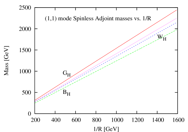
Figure 1: Variation of $G^{(1,1)}_{H}({\rm solid}),W^{3(1,1)}_{H}$ (small dash) and $B^{(1,1)}_{H}$ (large dash) masses (after incorporating the one loop radiative corrections) with $R^{-1}$. For comparison, $\frac{\sqrt{2}}{R}$ (dotted) has also been presented.

Conservation of momentum (along the extra dimensions) in the full theory, implies KK number conservation in the effective 4D theory. Beginning with the SM-like interactions in the 6D, (called the bulk interactions) one can obtain the KK-number as well as KK-parity conserving interactions, in 4D effective theory after compactification. However, one can generate KK number violating operators at one loop level, starting from the bulk interactions. Structure of the theory demands that these operators can only be on $(0,0,),~{}(0,L)$ and $(L,L)$ points of the chiral square. Bulk interactions being symmetric under KK-parity, operators generated by loops also conserve the KK-parity. These KK number violating operators are phenomenologically very important. A single non zero mode KK particle can be produced only via the KK number violating interactions. Thus the complete 4D effective Lagrangian can be written as:

$${\cal L}_{4D} = \int_{0}^{L}dx^{4}\int_{0}^{L}dx^{5}\{{\cal{L}}_{bulk}+\delta(x_{4})\delta(L-x_{5}){\cal{L}}_{2}+[\delta(x_{4})\delta(x_{5})+$$ (4)

$$+ \delta(L-x_{4})\delta(L-x_{5})]{\cal{L}}_{1}\}$$

${\cal{L}}_{bulk}$ includes 6D kinetic term for the quarks, leptons, $SU(3)_{C}\times SU(2)_{L}\times U(1)_{Y}$ gauge fields, a Higgs doublet, 6D Yukawa interactions of the quarks and leptons to the Higgs doublet, and a 6D Higgs potential. ${\cal{L}}_{1}$ and ${\cal{L}}_{2}$ contain KK number violating interactions. As for example, the lowest dimensional localized operator that involve $-ve$ chirality 6D quark field ($F_{-}$) appear in ${\cal{L}}_{p}$ (p = 1,2) as

$$\frac{C_{pF}}{2^{2}M_{s}^{2}}i\bar{F}_{-R}\Gamma^{\mu}D_{\mu}F_{-R}+(\frac{C_{pF}^{\prime}}{2^{2}M_{s}^{2}}i\bar{F}_{-R}\Gamma^{l}D_{l}F_{-L}+h.c)$$ (5)

where $\Gamma^{\mu}$ with $\mu=0,1,2,3$ and $\Gamma^{l}$ with $l=4,5$ are six anti-commuting $8\times 8$ matrices, $D^{\mu},D^{l}$ are 6D covarient derivative, $C_{pF},C_{pF}^{\prime}$ are dimensionless parameters, and $M_{s}$ is the cut-off scale. ${\cal{L}}_{1}$ and ${\cal{L}}_{2}$ also include 4D like kinetic terms for all 6D scalar and gauge fields and some part of 6D kinetic term. Contributions to those localized operators might be induced by physics above the cut-off scale. We assume that those UV generated localized operators are also symmetric under KK parity, so that the stability of the lightest KK particle which can be a promising dark matter candidate, is ensured. Loop contributions by the physics below cut-off scale $M_{s}$ are used to renormalize the localized operators. These contributions are calculated in [15] at one loop order. Assuming bare contributions at the cutoff scale $M_{s}$ can be neglected, RG evolution fixes the values of the $C$ parameters.

3 Interactions of adjoint scalars

In this section, we will discuss the possible interaction of a $(j,k)$-mode adjoint scalar. The interactions of spinless adjoints can be classified as KK number conserving and KK number violating interactions. KK number conserving interactions arise from the compactification of the bulk Lagrangian, where as, KK number violating interactions arise mainly due to the loops involving KK number conserving interactions.

3.1 KK-number conserving interactions

Tree-level interactions of adjoint scalars with zero and non-zero mode fermions arise from the 6D kinetic terms for the fermions. After compactification and integrating over the compactified co-ordinates one can obtain the 4D effective interactions:

$${\cal L}~{}\supset~{} - ig\delta_{0,1,3}^{(j_{1},k_{1})(j_{2},k_{2})(j_{3},k_{3})}r_{j_{2},k_{2}}^{*}r_{j_{3},k_{3}}\bar{\psi}_{+L}^{(j_{1},k_{1})}A_{H}^{(j_{2},k_{2})}\psi_{+R}^{(j_{3},k_{3})}$$ (6)

$$- ig\delta_{0,1,3}^{(j_{1},k_{1})(j_{2},k_{2})(j_{3},k_{3})}r_{j_{2},k_{2}}^{*}r_{j_{3},k_{3}}\bar{\psi}_{-R}^{(j_{1},k_{1})}A_{H}^{(j_{2},k_{2})}\psi_{-L}^{(j_{3},k_{3})}$$

$$+ h.c$$

$g$ is the gauge coupling for the gauge group in consideration and $r_{j,k}=(j+ik)/\sqrt{j^{2}+k^{2}}$. The above form of the interactions are valid both for $A_{H}^{(j,k)}$ being an abelian spinless adjoint field and non-abelian spinless adjoint with the replacement of $A_{H}^{(j,k)}~{}\rightarrow~{}T^{a}A_{H}^{a(j,k)}$. $T^{a}$’s are the gauge group generators corresponding to the representation of $\Psi_{\pm}$. Appearance of the the $\delta$-functions in the above expression ensure the conservation of KK-number. We list the relevant Feynman Rules arising from the above interactions in Fig.7 of Appendix A.

3.2 KK-number violating interactions

Starting with the KK number conserving bulk interactions of 2UED one can generate KK number violating operators via loop effects. As for example, a dimension 5 operator involving two zero mode fermions and a even KK parity (with $j+k$ even) $(j,k)$- mode spinless adjoint can be constructed in such a way.

We have listed the KK-number violating 2-point and 3-point functions in Fig.8 of Appendix A. The amplitude for $A_{H}^{(j,k)}\to\psi_{-R}^{(0,0)}\psi_{-R}^{(0,0)}$ is also calculated in Appendix B and is given by,

$${\cal M}=-i\frac{g}{M_{j,k}}\;(K_{C_{1\psi_{R}}C_{2\psi_{R}}}^{(j,k)}-K_{C_{1\psi_{R}}^{\prime}C_{2\psi_{R}}^{\prime}}^{(j,k)})\;\left[\bar{u}(p_{1})p\!\!/P_{R}u(p_{2})\right]$$ (7)

Defining $\tilde{C}^{f}_{j,k}~{}=~{}K_{C_{1\psi_{R}}C_{2\psi_{R}}}^{(j,k)}-K_{C_{1\psi_{R}}^{\prime}C_{2\psi_{R}}^{\prime}}^{(j,k)}$, one can parametrise $\tilde{C}^{f}_{j,k}=\tilde{\xi}_{f}\frac{1}{16\pi^{2}}Log(M_{s}^{2}/M_{j,k}^{2})$. $\tilde{\xi}_{f_{L,R}}$ are dimensionless parameters which fix the couplings of adjoint scalars with two zero mode fermions.

$$\tilde{\xi}_{q_{L}} = 4g_{s}^{2}+\frac{9}{4}g^{2}+\frac{3}{4}g^{\prime 2}Y_{q_{L}}^{2}$$

$$\tilde{\xi}_{q_{R}} = 4g_{s}^{2}+\frac{3}{4}g^{\prime 2}Y_{q_{R}}^{2}$$

$$\tilde{\xi}_{e_{L}} = \frac{9}{4}g^{2}+\frac{3}{4}g^{\prime 2}Y_{e_{L}}^{2}$$

$$\tilde{\xi}_{e_{R}} = \frac{3}{4}g^{\prime 2}Y_{e_{R}}^{2}$$ (8)

where $Y_{f}$ is the hypercharge of the corresponding fermion $f$. Spinless adjoints can also couple with two SM gauge bosons. These couplings are generated from finite 1-loop diagrams (Appendix B). The dimension-5 operators, involving a $(1,1)$ mode colour spinless adjoint and two SM gauge boson, are given by:

$$\textit{C}_{\gamma g}^{G}\;\epsilon^{\mu\nu\alpha\beta}\;Tr\left[G_{\mu\nu}\;A_{\alpha\beta}\;G^{(1,1)}_{H}\right]+\textit{C}_{Zg}^{G}\epsilon^{\mu\nu\alpha\beta}Tr[G_{\mu\nu}Z_{\alpha\beta}G^{(1,1)}_{H}]$$ (9)

The dimension-5 operators, involving a $(1,1)$ mode $U(1)$ or $SU(2)$ spinless adjoint $(V^{(1,1)}_{H})$ ($B_{H}^{(1,1)}~{}or~{}W_{H}^{3(1,1)}$) and two SM gauge bosons, are given by,

$$\textit{C}_{gg}^{V}\epsilon^{\mu\nu\alpha\beta}\;Tr\left[G_{\mu\nu}G_{\alpha\beta}V^{(1,1)}_{H}\right]+\textit{C}_{\gamma\gamma}^{V}\epsilon^{\mu\nu\alpha\beta}A_{\mu\nu}A_{\alpha\beta}V^{(1,1)}_{H}$$ (10)

$$+ \textit{C}_{\gamma Z}^{V}\epsilon^{\mu\nu\alpha\beta}A_{\mu\nu}Z_{\alpha\beta}V^{(1,1)}_{H}+\textit{C}_{ZZ}^{V}\epsilon^{\mu\nu\alpha\beta}Z_{\mu\nu}Z_{\alpha\beta}V^{(1,1)}_{H}$$

$$+ \textit{C}_{W^{+}W^{-}}^{V}\epsilon^{\mu\nu\alpha\beta}W^{+}_{\mu\nu}W^{-}_{\alpha\beta}V^{(1,1)}_{H}$$

where $G_{\mu\nu},~{}A_{\mu\nu},~{}Z_{\mu\nu}$ and $W^{\pm}_{\mu\nu}$ are the field strengths of gluon, photon, $Z$-boson and $W^{\pm}$-boson respectively. The values of the $C$ coefficients can be found in Appendix B. We have used $\alpha=1/128$ and $sin^{2}\theta_{W}=0.23$. The SM running of strong coupling constant (with $\alpha_{s}=0.1$ at a scale of 1 TeV) has been used. Yukawa couplings for all light quarks ($u,~{}d,~{}c,~{}s$) have been neglected. Top and bottom quark Yukawa couplings are taken to be 1 and 0.02 respectively. For quarks the resulting values of $\tilde{\xi}$ parameters at a scale about $0.5~{}\rm TeV$ are $\tilde{\xi}_{q_{L}}=6.82$, $\tilde{\xi}_{u_{R}}=6.02$ and $\tilde{\xi}_{d_{R}}=5.89$.

Following the same algorithm in Appendix-B, one can obtain dimension-6 operators involving two spinless adjoints and a gauge boson of the form:

$$A_{\mu\nu}\partial^{\mu}B_{H}^{(1,1)}\partial^{\nu}W_{H}^{3(1,1)}+Tr\left[G_{\mu\nu}\partial^{\mu}B_{H}^{(1,1)}\partial^{\nu}G_{H}^{(1,1)}\right]$$ (11)

$$+ Tr\left[G_{\mu\nu}\partial^{\mu}G_{H}^{(1,1)}\partial^{\nu}W_{H}^{3(1,1)}\right]+Z_{\mu\nu}\partial^{\mu}B_{H}^{(1,1)}\partial^{\nu}W_{H}^{3(1,1)}$$

However, first, second and the third operator vanish identically if we use equation of motion for photon and gluon respectively. Moreover the decay of $W_{H}^{3(1,1)}$ to a $B_{H}^{(1,1)}$ (can take place via the last one) and a massive SM gauge boson is kinematically forbidden for $R^{-1}$ values upto 1.5 TeV.

4 Decays of $(1,1)$-mode spinless adjoints

Until now the discussions about the couplings of the adoint scalars were more or less general about any $(j,k)$ mode adjoint. However, from this section we will focus specifically on the phenomenology of the $(1,1)$ mode adjoints.

$(1,1)$-mode spinless adjoint can decay into a lighter $(1,1)$-mode particle (kinematically possible only for $SU(3)$ and $SU(2)$ spinless adjoints) and one or two SM particles via the KK-number conserving couplings. This can also decay to a pair of SM fermions/gauge bosons via the KK-number violating interactions. In this section we compute the all such decay branching fractions of $(1,1)$- mode spinless adjoints using the interactions derived in the previous section.

4.1 Decays of $G_{H}^{(1,1)}$

As discussed, $G_{H}^{(1,1)}$ can decay to the SM quarks via loop induced operators. The amplitude for $G_{H}^{(1,1)}~{}\to~{}\bar{q}q$ is given by

$${\cal{M}}~{}=~{}-i\frac{g_{s}}{M_{j,k}}\bar{u}(p_{1})p\!\!/\left(\tilde{C}^{q_{R}}_{j,k}P_{R}+C^{q_{L}}_{j,k}P_{L}\right)u(p_{2})$$ (12)

Applying Dirac equation it is easy to see that the amplitude is proportional to quark mass. So $G_{H}^{(1,1)}$ predominantly decays into $t\bar{t}$ for $M_{G_{H}^{(1,1)}}>2m_{t}$. However, there are other dimension-5 operators which couple $G_{H}^{(1,1)}$ with a SM gluon and an electro weak gauge bosons. Since these couplings arise from finite 1-loop diagrams (Fig.10), they are suppressed by a logarithm compared to the $G_{H}^{(1,1)}q\bar{q}$ couplings. $G_{H}^{(1,1)}$ being heavier than the $U(1)$ gauge boson $B_{\mu}^{(1,1)}$, can decay into $B_{\mu}^{(1,1)}$ and a SM gluon. This coupling is also generated by finite 1-loop diagram and is thus suppressed.

We first consider the decay into $t\bar{t}$ and $b\bar{b}$. The widths can be computed in terms of the parameters $\tilde{\xi}_{q_{L}}$ and $\tilde{\xi}_{q_{R}}$ given in Eq.8. The decay width into $q\bar{q}$ is given by

$$\Gamma(G_{H}^{(1,1)}\to q\bar{q}) = \Gamma_{0}^{G_{H}}(\tilde{\xi}^{2}_{q_{L}}+\tilde{\xi}^{2}_{q_{R}})(\frac{m_{q}}{m_{G_{H}^{(1,1)}}})^{2}(1-\frac{4m_{q}^{2}}{m^{2}_{G_{H}^{(1,1)}}})^{\frac{1}{2}}$$ (13)

Where, $q$ can be $t$ or $b$ and $\Gamma_{0}^{G_{H}}~{}=~{}\frac{\alpha_{s}}{4}m_{G_{H}^{(1,1)}}\tilde{C}_{1,1}^{2}$

The decay width to $gB_{\mu}^{(1,1)},~{}gZ$ and $g\gamma$, induced by finite 1-loop effect, are as the following :

$$\Gamma(G_{H}^{(1,1)}\to B_{\mu}^{(1,1)}g) = \frac{\alpha_{s}^{2}\alpha}{32\pi^{2}cos^{2}\theta_{w}}(\sum_{\psi_{\pm}}\frac{Y_{\psi}}{2}\sigma_{\psi}A_{\psi}^{GB_{\nu}^{(1,1)}g})^{2}f_{G}(m_{B_{\nu}^{(1,1)}})$$

$$\Gamma(G_{H}^{(1,1)}\to gZ) = \frac{\alpha_{s}^{2}\alpha}{32\pi^{2}cos^{2}\theta_{w}sin^{2}\theta_{w}}f_{G}(m_{z})$$

$$\times (\sum_{\psi_{\pm}}[I^{3}_{\psi}-Q_{\psi}sin^{2}\theta_{w}]\sigma_{\psi}A_{\psi}^{GgZ})^{2}$$

$$\Gamma(G_{H}^{(1,1)}\to g\gamma) = \frac{\alpha_{s}^{2}\alpha}{32\pi^{2}}(\sum_{\psi_{\pm}}Q_{\psi}\sigma_{\psi}A_{\psi}^{Gg\gamma})^{2}f_{G}(0)$$ (14)

Where $f_{G}(m)~{}=~{}[(m^{2}_{G_{H}^{(1,1)}}-m^{2})/m_{G_{H}^{(1,1)}}]^{3}$ and $A_{\psi}$’s (in Eqs.14, 16 and 18) are defined in Eqs.B.3. It important to notice that for $M_{G_{H}^{(1,1)}}<350~{}GeV$ the dominant decay mode is $gZ$ rather than $b\bar{b}$. Although the $G_{H}^{(1,1)}b\bar{b}$ couplings is logarithmically enhanced but it is suppressed by $b$-quark mass.

Beside those two body decays, $G_{H}^{(1,1)}$ undergoes tree-level 3-body decays to $B_{H}^{(1,1)},~{}B_{\mu}^{(1,1)}$ or $W_{H}^{3(1,1)}$ and SM fermion anti-fermion pairs. Branching fractions of those decays are also presented in the Fig.2

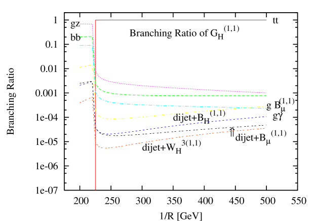
Figure 2: Branching Ratios of $G_{H}^{(1,1)}$. $M_{s}R=10$ has been assumed in the calculation

4.2 Decays of $B_{H}^{(1,1)}$

$B_{H}^{(1,1)}$ is the lightest $(1,1)$ mode KK particle. So, the decay $B_{H}^{(1,1)}$ via KK number conserving interactions are not kinematically allowed. It can decay to $f\bar{f}$ via dimension-5 operator in Eq.7. Since the coupling is proportional to the fermion mass, $B_{H}^{(1,1)}$ decay predominantly to $t\bar{t}$ for $m_{B_{H}^{(1,1)}}>2m_{t}$. The decay modes $b\bar{b}$ and $\tau\bar{\tau}$ are suppressed due to fermion mass. $B_{H}^{(1,1)}$ can also decay to two SM gauge bosons through dimension-5 operators Eq.10, generated from finite 1-loop contribution. However, these vertices are suppressed by a logarithm compared to $B_{H}^{(1,1)}f\bar{f}$ vertex.
The decay width to $t\bar{t},~{}b\bar{b}$ and $\tau\bar{\tau}$ are given by

$$\Gamma(B_{H}^{(1,1)}\to t\bar{t}) = 3\Gamma_{0}^{B_{H}}(\frac{1}{4}\tilde{\xi}^{2}_{t_{L}}+4\tilde{\xi}^{2}_{t_{R}})(\frac{m_{t}}{m_{B_{H}^{(1,1)}}})^{2}(1-\frac{4m_{t}^{2}}{m^{2}_{B_{H}^{(1,1)}}})^{\frac{1}{2}}$$

$$\Gamma(B_{H}^{(1,1)}\to b\bar{b}) = 3\Gamma_{0}^{B_{H}}(\frac{1}{4}\tilde{\xi}^{2}_{b_{L}}+\tilde{\xi}^{2}_{b_{R}})(\frac{m_{b}}{m_{B_{H}^{(1,1)}}})^{2}(1-\frac{4m_{b}^{2}}{m^{2}_{B_{H}^{(1,1)}}})^{\frac{1}{2}}$$

$$\Gamma(B_{H}^{(1,1)}\to\tau\bar{\tau}) = \Gamma_{0}^{B_{H}}(\frac{9}{4}\tilde{\xi}^{2}_{\tau_{L}}+9\tilde{\xi}^{2}_{\tau_{R}})(\frac{m_{\tau}}{m_{B_{H}^{(1,1)}}})^{2}(1-\frac{4m_{\tau}^{2}}{m^{2}_{B_{H}^{(1,1)}}})^{\frac{1}{2}}$$ (15)

Where, $\Gamma_{0}^{B_{H}}=\frac{\alpha}{18cos^{2}\theta_{w}}m_{B_{H}^{(1,1)}}\tilde{C}_{1,1}^{2}$. The decay widths of $B_{H}^{(1,1)}$ into two SM gauge bosons are as follows:

$$\Gamma(B_{H}^{(1,1)}\to gg) = \frac{\alpha_{s}^{2}\alpha}{8\pi^{2}cos^{2}\theta_{w}}(\sum_{\psi_{\pm}}\frac{Y_{\psi}}{2}\sigma_{\psi}A_{\psi}^{Bgg})^{2}f_{B}(0)$$

$$\Gamma(B_{H}^{(1,1)}\to\gamma\gamma) = \frac{\alpha^{3}}{16\pi^{2}cos^{2}\theta_{w}}(\sum_{\psi_{\pm}}\frac{Y_{\psi}}{2}Q_{\psi}^{2}\sigma_{\psi}A_{\psi}^{B\gamma\gamma})^{2}f_{B}(0)$$

$$\Gamma(B_{H}^{(1,1)}\to\gamma Z) = \frac{\alpha^{3}}{8\pi^{2}cos^{4}\theta_{w}sin^{2}\theta_{w}}f_{B}(m_{Z})$$

$$( \sum_{\psi_{\pm}}\frac{Y_{\psi}}{2}[I^{3}_{\psi}-Q_{\psi}sin^{2}\theta_{w}]Q_{\psi}\sigma_{\psi}A_{\psi}^{B\gamma Z})^{2}$$

$$\Gamma(B_{H}^{(1,1)}\to ZZ) = \frac{\alpha^{3}}{16\pi^{2}cos^{6}\theta_{w}sin^{4}\theta_{w}}f_{B}^{\prime}(m_{Z})$$

$$( \sum_{\psi_{\pm}}\frac{Y_{\psi}}{2}[I^{3}_{\psi}-Q_{\psi}sin^{2}\theta_{w}]^{2}\sigma_{\psi}A_{\psi})^{2}$$

$$\Gamma(B_{H}^{(1,1)}\to W^{+}W^{-}) = \frac{\alpha^{3}}{32\pi^{2}cos^{2}\theta_{w}sin^{4}\theta_{w}}f_{B}^{\prime}(m_{W})$$ (16)

$$( \sum_{\psi_{\pm}}\frac{Y_{\psi}}{2}\sigma_{\psi}A_{\psi})^{2}$$

Where, $f_{B}^{\prime}(m)~{}=~{}m_{B_{H}^{(1,1)}}^{3}[1-4m^{2}/m_{B_{H}^{(1,1)}}^{2}]^{3/2}$, and $f_{B}(m)=[(m^{2}_{B_{H}^{(1,1)}}-m^{2})/m_{B_{H}^{(1,1)}}]^{3}$. For $M_{B_{H}^{(1,1)}}<2m_{t}$, $B_{H}$ dominantly decays to a pair of gluons. For $M_{B_{H}^{(1,1)}}>2m_{t}$, beside $t\bar{t}$, the next dominant decay mode is $W^{+}W^{-}$. This is a consequence of large mass splitting of $(1,0)$ mode quarks and leptons as discussed in Appendix B. The different branching ratios of $B_{H}$ are presented in Fig.3.

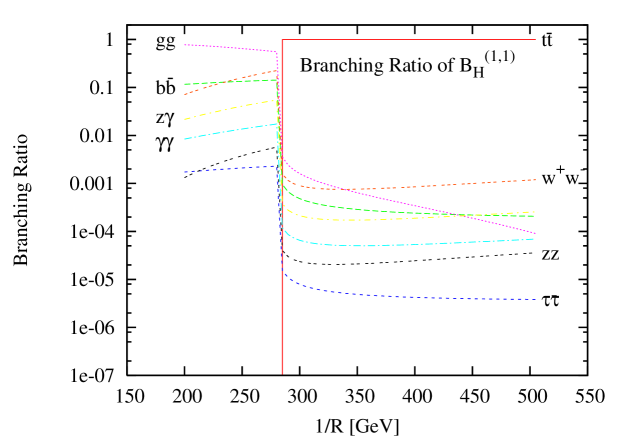
Figure 3: Branching Ratios of $B_{H}^{(1,1)}$ to pair of SM particles. $M_{s}R=10$ has been assumed in the calculation

4.3 Decays of $W_{H}^{3(1,1)}$

$W^{3(1,1)}_{H}$ is the next to the lightest $(1,1)$ mode particle. $W^{3(1,1)}_{H}$ can decay only into a pair of SM particles via KK number violating interactions mentioned before. The dominant decay mode is again into $t\bar{t}$ for $m_{W_{H}^{3(1,1)}}>2m_{t}$. $W^{3(1,1)}_{H}$ can decay to other SM fermion anti-fermion pairs but such decays are suppressed by the respective fermion masses. The decay width of $W^{3(1,1)}_{H}$ into $f\bar{f}$ is given by

$$\Gamma(W_{H}^{3(1,1)}\to f\bar{f})~{}=~{}C_{F}\Gamma_{0}^{W^{3}_{H}}\tilde{\xi}^{2}_{f_{L}}(\frac{m_{f}}{m_{W_{H}^{3(1,1)}}})^{2}(1-\frac{4m_{f}^{2}}{m^{2}_{W_{H}^{3(1,1)}}})^{\frac{1}{2}}$$ (17)

Where, $\Gamma_{0}^{W^{3}_{H}}=\frac{\alpha I_{3}^{2}}{2Sin^{2}\theta_{w}}m_{W_{H}^{3(1,1)}}\tilde{C}_{1,1}^{2}$ and $C_{F}$ is the quadratic casimir.

Apart from this decay, electrically neutral $(1,1)$ mode $SU(2)$ spinless adjoint can decay into two SM gauge bosons but these decays are again suppressed by a logarithm. The decay widths are given by

$$\Gamma(W_{H}^{3(1,1)}\to gg) = \frac{\alpha_{s}^{2}\alpha}{8\pi^{2}sin^{2}\theta_{w}}(\sum_{\psi_{+}}I_{\psi}^{3}\sigma_{\psi}A_{\psi}^{Wgg})^{2}f_{W}(0)$$

$$\Gamma(W_{H}^{3(1,1)}\to\gamma\gamma) = \frac{\alpha^{3}}{16\pi^{2}sin^{2}\theta_{w}}(\sum_{\psi_{+}}I_{\psi}^{3}Q_{\psi}^{2}\sigma_{\psi}A_{\psi}^{W\gamma\gamma})^{2}f_{W}(0)$$

$$\Gamma(W_{H}^{3(1,1)}\to\gamma Z) = \frac{\alpha^{3}}{8\pi^{2}cos^{2}\theta_{w}sin^{4}\theta_{w}}f_{W}(m_{Z})$$

$$( \sum_{\psi_{+}}I_{\psi}^{3}[I^{3}_{\psi}-Q_{\psi}sin^{2}\theta_{w}]Q_{\psi}\sigma_{\psi}A_{\psi}^{W\gamma Z})^{2}$$

$$\Gamma(W_{H}^{3(1,1)}\to ZZ) = \frac{\alpha^{3}}{16\pi^{2}cos^{4}\theta_{w}sin^{6}\theta_{w}}f_{W}^{\prime}(m_{Z})$$

$$( \sum_{\psi_{+}}I_{\psi}^{3}[I^{3}_{\psi}-Q_{\psi}sin^{2}\theta_{w}]^{2}\sigma_{\psi}A_{\psi}^{WZZ})^{2}$$

$$\Gamma(W_{H}^{3(1,1)}\to W^{+}W^{-}) = \frac{\alpha^{3}}{32\pi^{2}sin^{6}\theta_{w}}(\sum_{\psi_{+}}I_{\psi}^{3}\sigma_{\psi}A_{\psi}^{WW^{+}W^{-}})^{2}f_{W}^{\prime}(m_{W})$$ (18)

The previous definition of $f$ and $f^{\prime}$ functions holds here with proper change in spinless adjoint mass. The branching ratios are presented in Fig.4.

There are also tree-level 3-body decay of $W_{H}^{3(1,1)}$ into left-handed SM fermion anti-fermion pairs and $B_{H}^{(1,1)}$. As can be seen from Fig.4, those decay modes are very suppressed compared to others.

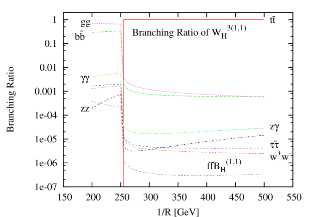
Figure 4: Branching ratios of $W^{3(1,1)}_{H}$. $M_{s}R=10$ has been assumed in the calculation

5 Production of $(1,1)$-mode Spinless Adjoints

We will first discuss the pair production of $(1,1)$-mode adjoint scalars. Production of $(1,0)$-mode scalars (in particular the $G_{H}^{(1,0)}$) was discussed in ref.[14]. We will also discuss the production of electroweak ($W^{3}_{H}$ and $B_{H}$) $(1,1)$-mode scalars along with $G_{H}$. Coupling of a pair of $G_{H}^{(1,1)}$ with a zero mode gluon, and coupling of a (1,1) mode quark with a zero mode quark and a $G_{H}^{(1,1)}$ arise from bulk interaction. We have estimated the following cross-sections : $\sigma(G_{H}G_{H})$, $\sigma(G_{H}B_{H})$, $\sigma(G_{H}W^{3}_{H})$, $\sigma(B_{H}B_{H})$, $\sigma(W^{3}_{H}W^{3}_{H})$, $\sigma(W^{3}_{H}B_{H})$ in proton proton collision at the LHC energies. CTEQ4L parton distribution functions [16] are used to numerically evaluate the above cross-sections. We have fixed the factorisation scale (for parton distribution functions) and scale of $\alpha_{s}$ (where relevant) at ${(1,1)}$ mode mass.

All the above cross-sections are presented in Fig.5. $G_{H}^{(1,1)}$ pair-production being a pure QCD process has a large cross-section at the LHC. Single $B_{H}^{(1,1)}$ or $W_{H}^{(1,1)}$ production along with a $G_{H}^{(1,1)}$ also have large cross-sections. On the other hand, pair productions of electroweak adjoint scalars are miniscule even for lower values of $R^{-1}$. Dominance of $G_{H}^{(1,1)}G_{H}^{(1,1)}$ pair production can be primarily attributed to contributions from the the gluon gluon initiated contributions. Gluonic contributions are absent in all other cases we have presented in above two figures. Apart from the $G_{H}^{(1,1)}G_{H}^{(1,1)}$ pair production, all other processes are only initiated by quarks and an anti-quarks. LHC, being a proton proton collider, anti-quarks can only arise from sea-excitation. Their densities also fall sharply with adjoint scalar masses.

$G_{H}^{(1,1)}$ pair production varies from a few pb to few fb, as we change $R^{-1}$ over a range from 200 to 1200 GeV. Once produced $G_{H}^{(1,1)}$ will decay dominantly to $t\bar{t}$, thus copiously producing 4 $t$-quarks. Distinguishing this signal from the SM background will be a challenging task. However, for $G_{H}^{(1,1)}$ masses below $2m_{t}$, it can decay to $gZ$, thus producing a spectacular 2-jet + 4 lepton signal.

Production cross-sections of $W_{H}^{(1,1)}$ and $B_{H}^{(1,1)}$ in association with $G_{H}^{(1,1)}$ are also presented in Fig.5a. $W_{H}^{(1,1)}$ ($B_{H}^{(1,1)}$) cross-sections varies from 100 (10) fb to 0.01 fb as we vary $R^{-1}$ from 200 to 1200 (1000) GeV.

Fig.5b, shows the pair production of electroweak adjoint scalars, namely $(1,1)$ mode of $W_{H}$ and $B_{H}$. These cross-sections are small and are comparable with the single productions of these scalars (discussed in the following).

Pair production of all these adjoint scalars via KK-number conserving interactions, result in $4t$ signal, once the scalar masses are greater than twice the top mass.

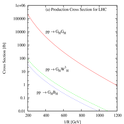
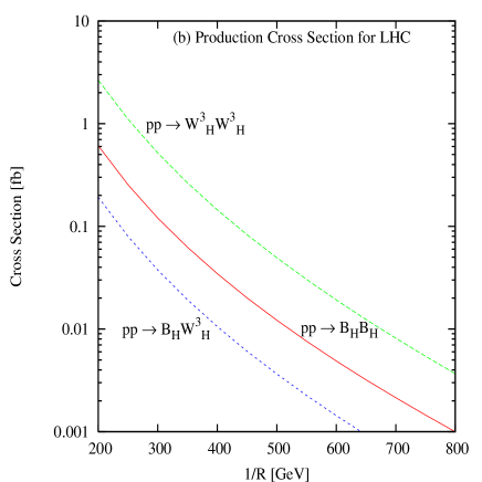
Figure 5: Pair production cross-sections for various $(1,1)$ mode adjoint scalars. CTEQ4L parton distributions are used to evaluate the cross-sections.

We will now briefly discuss the single production of adjoint scalars, $W^{(1,1)}_{3H}$ and $B^{(1,1)}_{H}$, the adjoints of the electro-weak gauge group. These can be produced at the LHC via gluon gluon fusion as well as in association with top-quark. However, $G^{(1,1)}_{H}$ cannot be produced via gluon gluon fusion due to $SU(3)$ symmetry. The only single production mode for this strongly interacting adjoint scalar is in association with a pair of $t$-quarks. This associated production rate is proportional to the fifth power of gauge couplings. As a result, the cross-sections, even for relatively lower values of $R^{-1}$, are not so promising. They also fall sharply with $R^{-1}$. This is primarily due to the direct $R^{-1}$ dependence of $G^{(1,1)}_{H}t\bar{t}$ couplings.

Resonance production cross-section of $W^{(1,1)}_{3H}$ and $B^{(1,1)}_{H}$ from $pp$ collision is given by

$$\sigma(pp\rightarrow V^{(1,1)}_{H}+X)=\frac{\pi^{2}}{36sm_{V_{H}}}\;\Gamma(V^{(1,1)}_{H}\rightarrow gg)\int_{\tau}^{1}\frac{dx}{x}\;g(x,m^{2}_{V})g(\frac{\tau}{x},m_{V}^{2})$$ (19)

s is the $pp$ center-of-mass energy square, $\tau$ is a dimensionless parameter : $\frac{m_{V_{H}}^{2}}{s}$. $g$’s are the gluon densities inside a proton.

In the previous section, we obtained the expressions for the various decay widths of the spinless adjoints. It is now straightforward to calculate the cross-sections using the above expression. We have presented the $W^{(1,1)}_{3H}$ and $B^{(1,1)}_{H}$ production cross-sections in Fig.6. CTEQ4L parton distributions have been used to numerically evaluate the cross-sections. Smallness of the cross-sections can be attributed to the narrow decay widths of these scalars into a gluon pair. The narrow decay widths of these electroweak adjoint scalars are evident in view of incomplete anomaly cancellation as explained in the Appendix B.

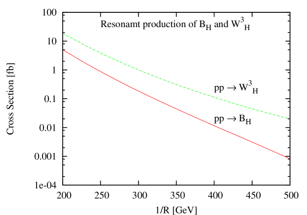
Figure 6: Resonant production cross-sections of $W^{3(1,1)}_{H}$ and $B^{(1,1)}_{H}$ at the LHC with $R^{-1}$.

6 Conclusion

To summarise, we have investigated the phenomenology of the adjoint scalars in an effective 4D theory, resulting from the compactification of Standard Model in 6 space time dimensions. These scalars arise from the 6th component of the gauge fields of the gauge groups $SU(3)$, $SU(2)$ and $U(1)$ respectively after compactification. Apart from KK-number conserving interactions which arise from the bulk, adjoint scalars have interactions with a pair of SM particles via KK-number violating but KK-parity conserving terms in the interaction Lagrangian. The later couplings arise via one-loop effects due to bulk interactions. Structure of the theory, in particular the chiral nature of compactifiation forces these effective couplings to be on the fixed points of the manifold. We have calculated these effective couplings involving the $(j,k)$ mode of the adjoint scalars ($G_{H}$, $W_{H}$ and $B_{H}$) with a pair of SM fields. The possible decays of $(1,1)$ mode scalars have been calculated. It is found that if kinematically allowed, they will dominantly decay to a pair of the heaviest fermions, namely the top-quark. We have calculated the pair production cross-section of the adjoint scalars in the context of Large Hadron Collider. Pair production of adjoint scalars involves only the KK-number conserving interactions. $G^{(1,1)}_{H}G^{(1,1)}_{H}$,$G^{(1,1)}_{H}W^{3(1,1)}_{H}$, $G^{(1,1)}_{H}B^{(1,1)}_{H}$ cross-sections are large. On the other hand $B^{(1,1)}_{H}W^{3(1,1)}_{H}$,$W^{3(1,1)}_{H}W^{3(1,1)}_{H}$, $B^{(1,1)}_{H}B^{(1,1)}_{H}$ pair productions at LHC are small. We have also computed the single production rates of $W_{H}^{3(1,1)}$ and $B_{H}^{(1,1)}$ via gluon gluon fusion which take place via KK-number violating interactions, at the LHC. $G^{(1,1)}_{H}$ cannot be produced singly via gluon gluon fusion. However, the single production cross-sections via KK-number violating interaction are in general small.

Acknowledgements KG acknowledges the support from Council of Scientific and Industrial Research, Govt. of India. AD is partially supported by Council of Scientific and Industrial Research, Govt. of India, via a research grant 03(1085)/07/EMR-II.

Appendix A : Relevant Feynman Rules

In this Appendix, we list the Feynman rules those are relevant for loop calculations. KK number conserving vertices involving a gauge boson or a spinless adjoint and two fermions are listed in Fig.7.

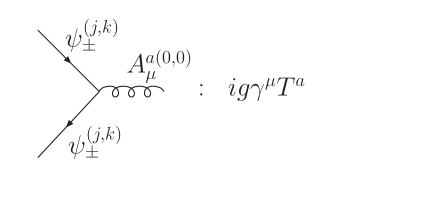
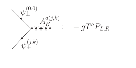
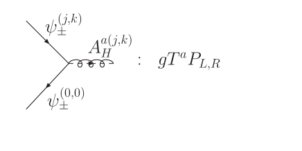
Figure 7: Feynman rules of KK-number conserving interactions arising from Eq.6. $g$ is the gauge coupling constant and $T^{a}$ is the generator of the relevant gauge group. For $U(1)$, $T^{a}$s should be replaced by $\frac{Y}{2}$.

Operators localized at the singular points, after compactification, give rise to the KK number violating 2-point and 3-point functions. These are listed in Fig.8. KK number violating 2-point functions induce kinetic and mass mixing between different $(j,k)$ modes. Corresponding 2-point and 3-point functions involving electro-weak gauge bosons can be easily inferred from those given in Fig.8. $K^{(j,k)}_{C_{1}C_{2}}$ in Fig.8 is defined as:

$$K^{(j,k)}_{C_{1}C_{2}}~{}=~{}\frac{2}{(\pi RM_{s})^{2}}(2C_{1}~{}+~{}(-1)^{j}C_{2})$$ (A.1)

$C_{1},~{}C_{2}$ are the dimensionless parameters, already introduced in Eq.5. In Appendix B, we will use these KK-number violating 2-point functions to compute the coupling of an even KK-parity spinless adjoint with two SM fermions.

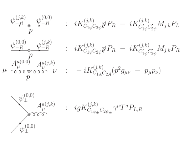
Figure 8: Feynman rules of KK-number violating interactions arising from compactification of fixed point operators.

Appendix B : KK-number violating Loop Induced Couplings

In this Appendix, we first compute $A_{H}^{(j,k)}\to\psi_{-R}^{(0,0)}\psi_{-R}^{(0,0)}$ amplitude. This kind of interactions are generated only by loop effects. One can construct dimension-5 operators which couples two zero mode fermions and a $(j,k)$-mode (with $j+k$ even) spinless adjoint, using the Feynman rules in Fig.7 and Fig.8. As for example, the amplitude for $B_{H}^{(j,k)}\to\psi_{-R}^{(0,0)}\psi_{-R}^{(0,0)}$ is given by

$${\cal M}=-ig^{\prime}\frac{Y_{\psi}}{2}\frac{1}{M_{j,k}}(K_{C_{1\psi_{R}}C_{2\psi_{R}}}^{(j,k)}-K_{C_{1\psi_{R}}^{\prime}C_{2\psi_{R}}^{\prime}}^{(j,k)})\;\left[\bar{u}(p_{1})p\!\!/P_{R}u(p_{2})\right]$$ (B.1)

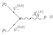
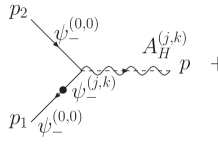
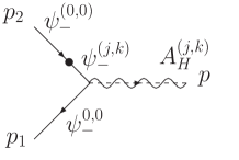
Figure 9: Vertices involving two zero mode fermions and a even KK parity $(j,k)$ mode spinless adjoint

Modulo the KK parity conservation, spinless adjoints can interact with two vector modes via finite 1-loop diagram. The coupling of a $(J_{1},K_{1})$ mode spinless adjoint with a $(J_{2},K_{2})$ mode gauge boson and a zero mode gauge boson is induced by the 1-loop diagram in Fig.10.

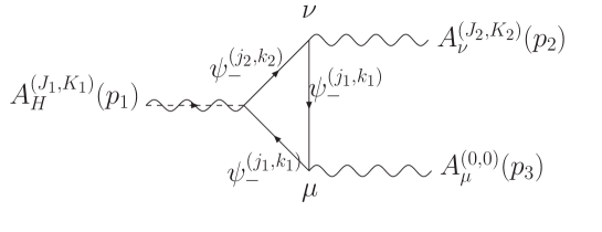
Figure 10: Effective vertex involving one SM and an even KK parity $(J_{2},K_{2})$ mode gauge boson with a even KK parity $(J_{1},K_{1})$ mode spinless adjoint.

The amplitude for $A_{H}^{(J_{1},K_{1})}\to A_{\nu}^{(J_{2},K_{2})}A_{\mu}^{(0,0)}$ is given by:

$${\cal M}=\frac{1}{4\pi^{2}}\times(Gauge~{}Couplings)\times A_{\psi}\epsilon^{\mu\nu\alpha\beta}\epsilon^{*}_{\nu}(p_{2})\epsilon^{*}_{\mu}(p_{3})p_{1\alpha}p_{2\beta}$$ (B.2)

where we have defined $A_{\psi}$ in the following way

$$A_{\psi} = \sum_{j_{1},k_{1}}\sum_{j_{2},k_{2}}A_{\psi}^{j_{1},k_{1};j_{2},k_{2}}$$

$$A_{\psi}^{j_{1},k_{1};j_{2},k_{2}} = m_{\psi}^{j_{1},k_{1};j_{2},k_{2}}(C_{12}-C_{11}-C_{0})-m_{\psi}^{j_{2},k_{2};j_{1},k_{1}}(C_{12}-C_{11})$$

$$m_{\psi}^{j_{1},k_{1};j_{2},k_{2}} = m_{j_{1},k_{1}}Re[r^{*}_{J_{1};K_{1}}r_{j_{1},k_{1}}(\delta_{013}^{j_{1},k_{1};J_{1},K_{1};j_{2},k_{2}}\delta_{103}^{j_{2},k_{2};J_{2},K_{2};j_{3},k_{3}}$$ (B.3)

$$- \delta_{013}^{j_{2},k_{2};J_{1},K_{1};j_{1},k_{1}}\delta_{000}^{j_{1},k_{1};J_{2},K_{2};j_{2},k_{2}})]$$

$C_{0},~{}C_{11},~{}C_{12}$ are the scalar and vector three point functions of ‘t Hooft, Passarino and Veltman [17] and “Gauge Couplings” in Eq.B.2 corresponds to the product of three gauge couplings (arising in Fig.10) times respective group theory factors. $C$ functions depend only on the three external masses and the three internal (fermionic) masses. The coefficient $m_{\psi}^{j_{1},k_{1};j_{2},k_{2}}$ survives for a finite set of $(j_{1},k_{1};j_{2},k_{2})$. As for example, only $(1,0)$-mode fermion contributes to the loop in the coupling of a $(1,1)$ mode spinless adjoint with two zero-mode gauge bosons. The possible combinations of $(j_{1},k_{1};j_{2},k_{2})$ in the coupling of a $(1,1)$ spinless adjoint to a $(1,1)$ vector mode and a zero-mode gauge boson, are: $(1,0;1,0)$, $(2,0;1,1)$, $(1,1;0,0)$ and $(1,1;2,0)$. After summing over such contributions, we find,

$${\cal M}=\frac{1}{4\pi^{2}}\epsilon^{\mu\nu\alpha\beta}\epsilon^{*}_{\nu}(p_{2})\epsilon^{*}_{\mu}(p_{3})p_{1\alpha}p_{2\beta}\times\sum_{\psi}(GaugeCouplings)\;\sigma_{\psi}A_{\psi}$$ (B.4)

The resulting dimension-5 operators, involving a $(1,1)$ mode spinless adjoint and two zero-mode gauge bosons, are given in Eqs.[9,10]. The $C$ coefficients arise in Eqs.[9,10] are given by,

(B.6)

Where $\sigma_{\psi_{\pm}}=\pm 1$, $Q_{\psi}$, $I^{3}_{\psi}$ and $Y_{\psi}$ are the electric charge, $3^{rd}$ component of isospin and hypercharge of the corresponding fermion $\psi$ respectively.

It is important to notice that the effective $A_{H}^{(J_{1},K_{1})}A_{\nu}^{(J_{2},K_{2})}A_{\mu}^{(0,0)}$ vertex is proportional to the gauge anomaly. So in the limit that all the fermions at each KK level are degenerate in mass, $A_{\psi}$ becomes independent of $\psi$ and all $C$ coefficients vanish identically due to exact anomaly cancellation. The mass splittings of KK fermions due to the radiative corrections thus play a very crucial role for the non-zero values of the $C$ coefficients. As for example, $\textit{C}_{W^{+}W^{-}}^{B}$ is stronger than all other $\textit{C}^{B}$’s. In case of $\textit{C}_{W^{+}W^{-}}^{B}$, anomaly cancellation takes place exactly between $(1,0)$ mode of 6D $+ve$ chirality quarks and lepton generations. Where as, for others cases, cancellation take place partially between the $(1,0)$ mode of 6D $+ve$ and $-ve$ chirality quarks and leptons. The mass splitting between the $(1,0)$ mode $+ve$ 6D chirality quarks and lepton generations is higher than the mass splitting between $(1,0)$ mode of 6D $+ve$ and $-ve$ chirality fermions [12]. Similar kind of argument can be given in favour of the small value of $\textit{C}_{W^{+}W^{-}}^{W^{3}}$ compared to all others.

References

- [1] I. Antoniadis, Phys. Lett. B 246, 377 (1990); N. Arkani-Hamed, S. Dimopoulous and G. Dvali, Phys. Lett. B 429, 263 (1998); I. Antoniadis, N. Arkani-Hamed, S. Dimopoulos and G. R. Dvali, Phys. Lett. B 436, 257 (1998).
- [2] L. Randall and R. Sundrum, Phys. Rev. Lett. 83, 3370 (1999); ibid 83, 4690 (1999).
- [3] T. Appelquist, H. C. Cheng and B. A. Dobrescu, Phys. Rev. D 64, 035002 (2001); H. C. Cheng, K. T. Matchev and M. Schmaltz, Phys. Rev. D 66, 056006 (2002).
- [4] K. Dienes, E. Dudas, T. Gherghetta, Nucl. Phys. B537, 47 (1999); K. Dienes, E. Dudas, T. Gherghetta, Phys. Lett. B 436, 55 (1998); G. Bhattacharyya, A. Datta, S. K. Majee and A. Raychaudhuri, Nucl. Phys. B760, 117 (2007).
- [5] G. Servant, T. Tait, Nucl. Phys. B650, 391 (2003); K. Kong. K. Matchev, J. High Energy Phys. 038, 0601, (2006).
- [6] B. Dobrescu, D. Hooper, K. Kong, R. Mahbubani; Jour. Cosmo. Astro. Phys. 0710, 012 (2007).
- [7] K. Agashe, N. G. Deshpande and G. H. Wu, Phys. Lett. B 514, 309 (2001); D. Chakraverty, K. Huitu and A. Kundu, Phys. Lett. B 558, 173 (2003); A. J. Buras, M. Spranger and A. Weiler, Nucl. Phys. B660, 225 (2003); A. J. Buras, A. Poschenrieder, M. Spranger and A. Weiler, Nucl. Phys. B678, 455 (2004); J. F. Oliver, J. Papavassiliou and A. Santamaria, Phys. Rev. D 67, 056002 (2003); T. Appelquist and B. A. Dobrescu, Phys. Lett. B 516, 85 (2001); K. Agashe, N. G. Deshpande and G. H. Wu, Phys. Lett. B 511, 85 (2001).
- [8] T. G. Rizzo and J. D. Wells, Phys. Rev. D 61, 016007 (2000); A. Strumia, Phys. Lett. B 466, 107 (1999); C. D. Carone, Phys. Rev. D 61, 015008 (2000); C. Macesanu, C. D. McMullen and S. Nandi, Phys. Rev. D 66, 015009 (2002); C. Macesanu, C. D. McMullen and S. Nandi, Phys. Lett. B 546, 253 (2002); H. C. Cheng, Int. J. Mod. Phys. A 18, 2779 (2003); A. Muck, A. Pilaftsis and R. Ruckl, Nucl. Phys. B687, 55 (2004); G. Bhattacharyya, P. Dey, A. Kundu and A. Raychaudhuri, Phys. Lett. B 628, 141 (2005); M. Battaglia, A. Datta, A. De Roeck, K. Kong and K. T. Matchev, J. High Energy Phys. 033, 0507, (2005); B. Bhattacherjee and A. Kundu, Phys. Lett. B 627, 137 (2005); J. M. Smillie and B. R. Webber, J. High Energy Phys. 069, 0510, (2005).
- [9] T. Appelquist, B. Dobrescu, E.Ponton, H. Yee, Phys. Rev. Lett. 87, 181802 (2001).
- [10] B. Dobrescu, E. Poppitz, Phys. Rev. Lett. 87, 031801 (2001).
- [11] B. Dobrescu, K. Kong, R. Mahbubani, J. High Energy Phys. 006, 0707, (2007).
- [12] G. Burdman, B. Dobrescu, E. Ponton, Phys. Rev. D 74, 075008 (2006).
- [13] A. Freitas, K. Kong, arXiv:0711.4124 (hep-ph).
- [14] B. Dobrescu, E. Ponton, J. High Energy Phys. 071, 0403, (2004).
- [15] E. Ponton, L. Wang, J. High Energy Phys. 018, 0611, (2006).
- [16] H. Lai et al., Phys. Rev. D 55, 1280 (1997).
- [17] G.’t Hooft, M. Veltman, Nucl. Phys. B153, 365 (1979); G. Passarino, M. Veltman, Nucl. Phys. B160, 151 (1979).