Batch kernel SOM and related Laplacian methods for social network analysis

Abstract

Large graphs are natural mathematical models for describing the structure of the data in a wide variety of fields, such as web mining, social networks, information retrieval, biological networks, etc. For all these applications, automatic tools are required to get a synthetic view of the graph and to reach a good understanding of the underlying problem. In particular, discovering groups of tightly connected vertices and understanding the relations between those groups is very important in practice. This paper shows how a kernel version of the batch Self Organizing Map can be used to achieve these goals via kernels derived from the Laplacian matrix of the graph, especially when it is used in conjunction with more classical methods based on the spectral analysis of the graph. The proposed method is used to explore the structure of a medieval social network modeled through a weighted graph that has been directly built from a large corpus of agrarian contracts.

, , , and

1 Introduction

Complex networks are large graphs with a non trivial organization. They arise naturally in numerous context [7], such as, to name a few, the World Wide Web (which gives a perfect example of how large and complex such a network may grow), metabolic pathways, citation networks between scientific articles or more general social networks that model interaction between individuals and/or organizations, etc.

Complex networks share common properties that have allowed the emergence of mathematical descriptions such as small world graphs or power law graphs. The structure of these graphs often gives some keys to understand the complex network underlined. To study such a structure, one often begins with a metrology process applied to the graph that describes the degree distribution, the number of components, the density, etc. The second step consists in the search of subgraphs that have particular adjacency, in particular highly connected parts of the graph which are at the same time lightly connected between them. Such parts are called communities [41, 13]. More recently, several directions have been explored to go further in modelling large real networks, taking into account their dynamics [47], the attributes of the data [35], a more formal definition of the communities [42, 38, 37], or the relations between communities [40]. However, it should be noted that dealing with very large graphs (millions of vertices) is still an open question (see [9] for an example of an efficient algorithm to explore that kind of data sets).

Several ways have been explored to cluster the vertices of the graph into communities [43] and some of them have in common the use of the Laplacian matrix. Indeed, there are important relationships between the spectrum of the Laplacian and the graph invariants that characterize its structure (see, e.g. [32, 33]). These properties can be used for building, from the eigen-decomposition of the Laplacian, a similarity measure or a metric space such that the induced dissimilarities between vertices of the graph are related to its community structure (see [13], among others). The Laplacian matrix also appears when the vertices of the graph are clustered by the optimization of a graph cut quality measure: optimizing such a measure is generally a NP-complete problem but using the properties of spectrum of the Laplacian provides a relaxation based heuristic solution with a reasonable complexity [1].

In the present paper, the properties of the Laplacian are also used to identify and map communities, both in a rather classical way and with a recently proposed batch version of the kernel Self Organizing Map (SOM). The combination of those tools gives complementary views of a social network. The spectral based approach extracts a specific type of communities for which interpretation biases are limited, but which cover only part of the graph (e.g., one third of the vertices in the studied graph). The SOM solution gives a global map of the vertices clustered into more informal communities, for which a link analysis must be done with care. Combining the analysis of these classifications helps in getting some global results while limiting the risk of false interpretation.

In both cases, the communities’ organization is associated to a two dimensional representation that eases interpretation of their relations. It should be noted that these representations are not intended to compete with those coming from the large field of graph drawing [12, 23]: the goal in this paper is not to draw the whole graph but to extract a community structure and to provide a sketch of the organization of these small homogeneous social groups.

The rest of this paper is organized as follows. Section 2 defines perfect communities and uses spectral analysis of the Laplacian to identify them. An alternative and complementary approach is described in Section 3, where a kernel is derived from the Laplacian via a form of regularization. This kernel is used in Section 4 to implement a batch kernel SOM which builds less perfect communities and maps them on a two dimensional structure that respects their relationships. Section 5 is dedicated to an application of the proposed methods to a social network that models interactions between peasants in the French medieval society. The historical sources (agrarian contracts) are first presented together with the corresponding social network model. Methods proposed in Sections 2 and 4 are then applied to this graph. Results are compared and confronted to prior historical knowledge.

2 Clustering through the search of perfect communities

Understanding the structure of a large network is a major challenge. Fortunately, many real world graphs have a non uniform link density: some groups of vertices are densely connected between them but sparsely connected to outside vertices. Identifying those communities is very useful in practice [38] as they can provide a sort of summary which can in turn be analyzed more easily than the original graph, especially when human expertise is requested. However, there is no consensus on a formal definition of a community (see e.g., [41, 43]). In the context of visualization, a particular (and somehow restrictive) type of communities, the so called perfect communities, leads to interesting results. In addition, this precise form of communities, easy to define and understand, may be viewed as the elementary block of the communities, in their general meaning.

A perfect community of a non-weighted graph is a complete subgraph (in such a subgraph all vertices are pairwise linked by an edge), with at least $2$ vertices, and such that all its vertices have exactly the same neighbors outside the community. The perfect communities of a weighted graph are obtained as the perfect communities of its induced non-weighted graph (i.e., of the graph having same vertices and edges but no weights on the edges). In [49], Van den Heuvel and Pejic proposed that particular form of community for non-weighted graphs in the case of frequency assignment problems. They give a different definition for weighted graphs; this last one was not followed because it appears as too restrictive for more general graphs such as those coming from social networks.

A nice advantage of perfect communities over looser ones is that they have simple non ambiguous visual representations. Indeed perfect communities can be represented by simple glyphs (circles for instance) together with their connections to other perfect communities without loosing information: the nodes in a perfect community are fully connected (hence each simple glyph symbolizes a complete subgraph) and share the same connections with the outside of the community (hence the unique representation of these connections by a simple link between two glyphs).

However, perfect communities don’t provide a complete summary of a graph. One of their main weaknesses is that, on real applications, the set of perfect communities can contain only a part (and sometimes a little part) of the whole graph. Moreover, some of the vertices that don’t belong to a perfect community can play a central role in the structure of the social network. Two parameters are usually used in social network analysis to characterize these important vertices: high degree and high betweenness measure (the definition is given below).

The vertices with the highest degrees are likely to have a main role in the graph as they are linked to a large number of other vertices. These vertices may appear in a rich-club [56] if it exists. The rich-club occurs when the vertices with highest degree form a dense subgraph with a small diameter. The diameter of a graph is the longest of the shortest path between any two given vertices of a graph and the density of a graph is the ratio beetwen the number of its edges and the number of the total possible edges. The construction of a rich-club starts from the highest degree vertices which are totally connected and follows by adding the next vertices in the decreasing order of their degrees. The process stops when the diameter reaches the fixed limit or when the density sharply decreases. In practice, the chosen limit for the diameter of the rich club is very small: for a graph having several hundred of vertices, as the one studied in Section 5, a diameter of 2 gives satisfactory results. As the rich club is a subgraph with a small diameter and a high density and as it shares many connections with the other vertices of the graph, it can be seen as a set of people having a main social role by knowing almost everybody in the community.

All the vertices of the graph don’t belong to a perfect community or to the rich club and some of them can still be important to obtain a good summary of the graph. Another interesting feature to localize relevant vertices is to look at the betweenness measure of the vertices. The betweenness measure of a vertex is the frequency of the shortest paths of any two vertices of the graph in which this vertex occurs. These vertices also have a main role as they are essential to connect the whole graph. In social networks, they can be seen as mediating persons that link together subgroups that would be otherwise unrelated.

The number of high betweenness vertices is chosen according to the following heuristic. Vertices are sorted in decreasing order of betweenness and the number of connected components of each subgraph $\mathcal{S}_{k}$ induced by the perfect communities, the rich-club and the first $k$ vertices with highest betweenness measure is computed. In general, the decrease of this number with $k$ is non uniform: sharp drops are separated by constant (flat) regions (see Figure 3 for an example). As important vertices are those that significantly reduce the number of connected components, it seems logical to consider a value of $k$ that lies just after a significant drop. The actual selection of $k$ remains however a matter of compromise as there are generally several significant decreases in the number of components: adding too much nodes will clutter the visualization while leaving out too many will miss some important individuals. Section 5.3 provides an example of such compromise. The final set of selected vertices are called central vertices.

Adding the rich-club and the central vertices to perfect communities enhances the coverage of the original graph while maintaining an easy visual representation. The first step consists in using adding glyphs for central vertices. As already explained above, links from a perfect community to any vertex is unambiguous and therefore the edges between perfect communities and central vertices (as well as between those vertices) can be added without difficulty. The only compromise concerns the rich-club. It is also represented by a specific glyph which does not show therefore its substructure. Another simplification is used for links: an edge between the rich-club and any other element (a central vertex or a community) summarizes a possibly complex link structure.

Perfect communities are not only easy to visualize; their computation is also straightforward, as described below. Let us first introduce some notations. $\mathcal{G}$ denotes a connected graph with vertices $V=\{x_{1},\ldots,x_{n}\}$ and a set of undirected edges $E$, with positive weights, $w_{i,j}=w_{j,i}$ ($w_{i,j}=0$ is equivalent to $\{x_{i},x_{j}\}\notin E$). The degree of a vertex $x_{i}$ is denoted $d_{i}=\sum_{j=1}^{n}w_{i,j}$.

The structure of $\mathcal{G}$ can be summarized through a symmetric $n\times n$ matrix called the Laplacian of ${\mathcal{G}}$. This matrix has been intensively studied the past years because many important structural and topological properties can be deduced from it. The Laplacian of ${\mathcal{G}}$ is defined as the positive and semi-definite matrix $L=(L_{i,j})_{i,j=1,\ldots,n}$ such that

$$L_{i,j}=\left\{\begin{array}[]{ll}-w_{i,j}&\textrm{ if }i\neq j,\\ d_{i}&\textrm{ if }i=j.\end{array}\right.$$

We will also consider the Laplacian, denoted by $\widetilde{L}$, of the non-weighted graph induced by $\mathcal{G}$, $\widetilde{\mathcal{G}}$.

Spectral properties of the Laplacian can be used to cluster the vertices of a graph. First of all, it is well known that the eigenvalue 0 is related to the minimum number of connected subgraphs in ${\mathcal{G}}$ [32]. In the same way, a spectral analysis of the Laplacian allows one to find perfect communities, using the following property (a set of vertices is called non-stable if it contains at least two adjacent vertices):

Theorem 1 ([49])

A non-stable set $\mathcal{S}$ of vertices is a perfect community if and only if there is a non-zero eigenvalue, $\lambda$, of $\widetilde{L}$ whose multiplicity is at least $k-1$ and such that the $k-1$ associated eigenvectors vanish for the same $n-k$ coordinates.

Then, the cardinal of $\mathcal{S}$ is $k$, the coordinates for which the $k-1$ eigenvectors are not 0 represent the vertices belonging to $\mathcal{S}$ and $\lambda=d+1$ where $d$ is the degree of a vertex of $\mathcal{S}$.

As a consequence, looking at null coordinates of the eigenvectors of $\widetilde{L}$ is a simple and efficient way to extract perfect communities. Moreover, we also have the following property, that will help to understand the link between this approach and the well-known spectral clustering method:

Corollary 2

If a set of vertices, $\mathcal{S}$, is a perfect community then the $n-k+1$ eigenvectors that do not define $\mathcal{S}$ have constant coordinates for the indices of the vertices of $\mathcal{S}$.

Proof   Without loss of generality, ${\mathcal{S}}$ is renumbered as ${\mathcal{S}}=\{1,\ldots,k\}$. An eigenvector $u$ defining $\mathcal{S}$ can be written as $u=(u_{1},...,u_{k},0,0,...,0)$. Let $z=(z_{1},...,z_{k},z_{k+1},...,z_{n})$ be an eigenvector that does not define $\mathcal{S}$ and note $\tilde{u}=(u_{1},...,u_{k})$, $\tilde{z}=(z_{1},...,z_{k})$. As $\widetilde{L}$ is symmetric, $z$ is orthogonal to the $k-1$ eigenvectors that define $\mathcal{S}$ so $\tilde{z}$ is orthogonal to the $k-1$ vectors $\tilde{u}$ for $u$ defining $\mathcal{S}$. But $u$ is an eigenvector of $\widetilde{L}$, so it is orthogonal to the vector $\mathbf{1}_{n}=(1,1,\ldots,1)$ (related to the eigenvalue 0) and so, $\tilde{u}$ is orthogonal to the vector $\mathbf{1}_{k}$ in $\mathbb{R}^{k}$. The orthogonal complement, in $\mathbb{R}^{k}$, of the vector space spanned by the $k-1$ vectors $\tilde{u}$ has dimension one and is spanned by $\mathbf{1}_{k}$; it follows that $\tilde{z}$ is co-linear to $\mathbf{1}_{k}$ which concludes the proof.

3 Similarity measures built from the Laplacian

Some weaknesses of a representation by perfect communities are the absence of a lot of vertices (for instance, only 35 % of the whole graph belongs to a perfect community in the social network studied in Section 5) and the presence of a lot of very small communities. Moreover, some relevant groupings of perfect communities might be missed and a bias of the interpretation can occur from these lacks. In this sense, the definition of perfect communities gives a too restrictive clustering of the vertices. It is therefore reasonable to complement it with the help of another clustering algorithm chosen in the numerous methods proposed for this task [43]. A broad class of those methods consists in building a (dis)similarity measure between vertices that capture the notion of community and then on applying an adapted clustering algorithm to the dissimilarity matrix.

To pursue this goal, this section introduces existing similarity measures based on the Laplacian. Section 3.1 explains how to build a similarity measure that is able to separate communities from each others and Section 3.2 follows a similar idea to define a kernel that maps the vertices in a high dimensional space. The purpose of the those sections is to emphasize the links and also the differences between the eigenvalue approach described in the previous section, the usual “spectral clustering” approach and the well-known diffusion kernel which can be considered as a smooth spectral clustering.

3.1 From almost perfect communities to graph cuts

One way to obtain an optimal clustering of the vertices of a graph is to minimize the following graph cut quality measure

$$\text{cut}({\mathcal{S}}_{1},\ldots,{\mathcal{S}}_{p})=\sum_{i=1}^{p}W({\mathcal{S}}_{i},{\mathcal{G}}\setminus{\mathcal{S}}_{i}),$$

where ${\mathcal{S}}_{1},\ldots,{\mathcal{S}}_{p}$ is a partition of $V$ (for a chosen $p$ in $\mathbb{N}^{*}$), and where $W(S,S^{\prime})=\sum_{i\in S,j\in S^{\prime}}w_{i,j}$ for two given sets of vertices $S$ and $S^{\prime}$ included in $V$. This optimization problem is NP complete for $p>2$ but it can be relaxed into a simpler problem (see, e.g., [53]):

$$\min_{H\in\mathbb{R}^{n\times p}}\text{Tr}(H^{T}LH)\text{ subject to }H^{T}H=\mathbb{I}_{p}.$$ (1)

The key point in the relaxation approach is to extend the search space from a discrete set in which the coefficients of $H$ define a partition of $\{1,\ldots,n\}$, to $\mathbb{R}^{n\times p}$.

For a connected graph, the solution of the relaxed problem is the matrix $H$ which contains the $p$ eigenvectors associated to the $p$ smallest positive eigenvalues of $L$ as columns. Of course, the real-valued solution provided by the matrix $H$ has to be converted into a discrete partition of $p$ clusters. A usual way to do do is to consider the solution matrix $H$ as a way to map vertices of the graph in $\mathbb{R}^{p}$ as follows:

$$F_{L}:x_{i}\in V\rightarrow(h^{(1)}_{i},\ldots,h^{(p)}_{i})\in\mathbb{R}^{p},$$ (2)

where $(h^{(j)})_{j}$ is an orthonormal set of eigenvectors associated to the $p$ smallest positive eigenvalues $(\lambda_{j})_{j=1,\ldots,p}$ ($h^{(j)}_{i}$ denotes the $i^{\text{th}}$ coordinate of the $j^{\textrm{th}}$ smallest positive eigenvalue). Then a standard clustering algorithm in $\mathbb{R}^{p}$ (e.g., the $k$-means algorithm) is applied to the mapped nodes (this can been seen as a clustering of the rows of $H$), leading to one variant of spectral clustering.

This method is strongly related to perfect communities calculation. Corollary 2 shows that vertices that belong to the same perfect communities have the same coordinates for many eigenvectors. As a consequence, any clustering algorithm applied on nodes mapped via $F_{L}$ will tend to gather vertices from a perfect communitiy in the same cluster. In this sense, spectral clustering can be seen as a relaxed version of the search of perfect communities.

It should be noted that the spectral clustering method summarized above gives equal weights to the first $p$ eigenvectors of the Laplacian, whereas the smaller the eigenvalue is, the more important the corresponding eigenvector is. Moreover, only the first $p$ eigenvalues are used and, hence, this approach doesn’t use the entire information provided by the Laplacian. To avoid these problems, a regularized version of the Laplacian can be used, as shown in the following section.

3.2 Diffusion kernel

In [46], the authors investigate a family of kernels on graphs based on the notion of regularization operators: a regularization function is applied to the Laplacian and gives a family of matrices that are also kernels on $V\times V$. In the present paper, we focus on the diffusion kernel:

Definition 3

The diffusion matrix of the graph ${\mathcal{G}}$ for the parameter $\beta>0$ is $D^{\beta}=e^{-\beta L}$.

The diffusion kernel of the graph $\mathcal{G}$ is the function

$$K^{\beta}:(x_{i},x_{j})\in V\times V\rightarrow D^{\beta}_{i,j}\in\mathbb{R}$$

The diffusion matrix is easy to compute for graphs having less than a few hundred of vertices by the way of an eigen-decomposition of the Laplacian: if $(h^{(i)})_{i=0,\ldots,n-1}$ are orthonormal eigenvectors associated to the eigenvalues $0=\lambda_{0}<\lambda_{1}\leq\lambda_{2}\leq\ldots\leq\lambda_{n-1}$ of $L$, then

$$D^{\beta}=\sum_{k=0}^{n-1}e^{-\beta\lambda_{k}}h^{(k)}{h^{(k)}}^{T}.$$ (3)

This diffusion kernel has been intensively studied through the past years. In particular, [29] shows that this kernel is the continuous limit of a diffusion process on the graph: $K^{\beta}(x_{i},x_{j})$ can be viewed as the value of the energy obtained in vertex $x_{j}$ after a time tending to infinity if energy has been injected in vertex $x_{j}$ at time 0 and if diffusion is continuously done among the edges of the graph. In this case, $\beta$ is related to the intensity of the diffusion (see also [8] for a complete description of the properties of this operator).

It is easy to prove that the kernel $K^{\beta}$ is symmetric and definite positive. Then, from Aronszajn’s Theorem [4, 6], there is a Reproducing Kernel Hilbert Space (RKHS), $({\mathcal{H}}_{\beta},\langle.,.\rangle_{\beta})$, called the feature space, and a mapping function, $\phi_{\beta}:V\rightarrow{\mathcal{H}}_{\beta}$ such that:

$$\textrm{for all }i,j,\ \langle\phi_{\beta}(x_{i}),\phi_{\beta}(x_{j})\rangle_{\beta}=K^{\beta}(x_{i},x_{j}).$$

As in the previous section, this mapping provides a way to apply standard clustering algorithms to the vertices of a graph, simply by working on their mapped values. In addition, a kernel trick can be used in many cases to avoid calculating explicitly the mapping (see Section 4.3 for details).

Equation (3) shows that the mapping induced by the kernel is equivalent to the following one:

$$F_{K}^{\beta}:x_{i}\in V\rightarrow(h^{(1)}_{i},\ldots,h^{(n)}_{i})\in(\mathbb{R}^{n},\langle.,.\rangle_{n}^{\beta}),$$ (4)

where $\mathbb{R}^{n}$ is considered with a specific inner product given by $\langle z,z^{\prime}\rangle_{n}^{\beta}=\sum_{k=0}^{n-1}e^{-\beta\lambda_{k}}z_{k}z^{\prime}_{k}$ for all $z$ and $z^{\prime}$ in $\mathbb{R}^{n}$.

Once again, as stated by Corollary 2, the vertices that belong to the same perfect community have very close images by $F_{K}^{\beta}$. However the embedding provided by $F_{L}$ (see equation (2)) uses only a part of the spectrum and will therefore loose some neighborhood informations. For example, vertices that belong to two different perfect communities can be indistinguishable. On the contrary, $F_{K}^{\beta}$ uses the whole eigen-decomposition but with a modified metric that contains non local information.

This approach is very flexible because the parameter $\beta$ permits to control the degree of smoothing: a small value of $\beta$ regularizes heavily and totally forbid to cluster together two vertices that are not directly linked to each others whereas a large $\beta$ allows to cluster vertices that are not directly connected but share a large number of common neighbors. This makes this kernel an attractive tool which is quite popular in the computational biology area where it has been used with success to extract pathway activity from gene expression data through a graph of genes [50, 45].

4 Kernel SOM for clustering the vertices of a graph

4.1 Motivations for the use of the SOM algorithm

Our purpose is to provide a description of the graph by clustering its vertices into relevant communities. However, clustering alone doesn’t always provide a clear picture of the global structure of a graph. As already mentioned, on the one hand, perfect communities are easy to understand but generally don’t cover the whole graph, while, on the other hand, clusters that are not perfect communities have complex relations one to another: a link between two clusters hides a potentially complex link structure between individuals in those clusters. A solution to circumvent those problems is to cluster the vertices of the graph in a way that both leads to imperfect communities but also takes into account relations between clusters.

To achieve these goals, one can leverage the topology preservation properties of the Self Organizing Map (SOM). This algorithm, first introduced by Kohonen [27], is an unsupervised method that performs at the same time a clustering and a non linear projection of a dataset. The SOM is based on a set of models (also called neurons or units) arranged according to a low dimensional structure (generally a regular grid in one or two dimensions). The original data are partitioned into as many homogeneous clusters as there are models, in such a way that close clusters (according to the prior structure) contain close data points in the original space.

The analysis of the vertices of a graph with a SOM will therefore provide a type of relaxed communities (the clusters) arranged in a way that is consistent with the link structure of the members of those communities, as long as the graph structure can be turned into a topology that the SOM will preserve.

4.2 SOM for non vector data

The standard SOM algorithm uses the euclidean structure of the data space and therefore cannot be applied directly to vertices of a graph. As non vector data arise naturally in many real world problems, adapted variants of the SOM have received a lot of attention in the past ten years. It should first be noted that the general structured data framework proposed in [21] cannot be applied to vertices of a graph: the framework is adapted to the case where each observation is a whole graph, not to the one that focuses on the nodes of a single graph.

A possible solution in this situation (explored in [51]) would be to use one of the variants of the Median SOM (also called the dissimilarity SOM, see [2, 26, 25, 28, 14]). Members of this class of algorithms can be applied to any dataset on which a dissimilarity measure can be defined: numerous dissimilarity measures for graph nodes have been proposed for graph clustering (see [43]) and could therefore be used with a dissimilarity SOM. Those SOM algorithms are based on a generalization of the notion of center of mass called a generalized median (fast implementations are available [10]). Another variant of the SOM for dissimilarity data, based on mean field annealing, could also be used [17, 18], as well as the recently introduced relational topographic mappings [19, 20].

The solution proposed in this paper is to rely on a kernelized version of the SOM: this is a natural choice in the sense that graphs are well described by their Laplacian and the corresponding heat kernels. As shown in [52], if the dissimilarity between objects is defined via a kernel, the median SOM is a type of constrained kernel SOM. Moreover, the constraints of the median SOM generally induce maps of lesser quality than those obtained by the kernel version. Further links between both approaches are outlined in [19, 20].

In the proposed kernel approach, detailed in the next paragraph, the vertices are first implicitly mapped into a feature space whose geometry reflects the graph structure. This implicit mapping is performed via the so called “kernel trick”, by using the diffusion kernel. Then, a batch SOM is applied in this space to perform a nonlinear projection of the vertices and, at the same time, a clustering, that will both respect the topology of the feature space and therefore of the graph.

An alternative (and in fact quite similar) solution would be to rely on an embedding, i.e., on an explicit mapping of the nodes of the graph to $\mathbb{R}^{p}$, exactly as this is done in the spectral clustering approach (see [11, 16, 53]). Rather than applying a $k$-means algorithm to the vector representation of the vertices obtained via the mapping $F_{L}$ (see equation (2)), one can simply use a standard SOM. For the application studied in this paper (the social network presented in Section 5), this solution performed poorly. While the overall organization of the obtained map was good, the clusters were much more unbalanced: a large cluster contained two third of the vertices, while other clusters were quite small (one or two vertices). This is not very surprising as the heat kernel helps to distinguish between vertices that could seem similar if they are represented by the information restricted to the smallest eigenvectors of the Laplacian (as explained in Sections 3.1 and 3.2).

Nevertheless, it should be noted that the important aspect of the proposed method is to rely on an adapted variant of the Self-Organizing Map to perform at the same time graph clustering and graph visualization. In the particular application studied in Section 5, the heat kernel (and therefore the batch kernel SOM) gives interesting results. In other applications, better results might be obtained with other kernels, with dissimilarities (via a dissimilarity SOM) or with embedding (via a standard SOM). The numerous SOM variants provide a general framework for graph mining: the present article explores only one of its possible concrete implementation.

4.3 Batch kernel SOM

Several kernelized version of the SOM have been proposed [30, 3, 52]. The present paper uses a batch version of the kernel SOM proposed in [52, 20]. An advantage of the batch kernel SOM, with respect to the stochastic versions proposed before, is that the former generally converges much faster than the latter.

As stated above, the kernel batch SOM first maps the original data into a high-dimensional Hilbert space $\mathcal{H}$ via a feature map $\phi$. Then, the standard batch SOM is applied to the mapped data. As with most kernelized algorithms, the mapping has not to be explicitly carried out. The batch SOM can be rewritten in such a way to use only the inner product of the Hilbert space: rather than defining $\mathcal{H}$ and $\phi$, one has only to specify a kernel $K$ on the original data set, as this generates an associated Reproducing Kernel Hilbert Space.

Let us first describe the batch SOM on the mapped data. The prior structure consists in $M$ neurons. The distance between neurons $i$ and $j$ in the prior structure is denoted $h(i,j)$. It is transformed into a neighborhood function via a decreasing function $R$, from $\mathbb{R}^{+}$ to $\mathbb{R}^{+}$, with $R(0)=1$ and $\lim_{s\rightarrow+\infty}R(s)=0$. The influence of the grid is annealed through time: at iteration $l$, the algorithm uses a function $R^{l}$, based on $R$, that is more and more concentrated in $0$.

At iteration $l$, neuron $j$ is associated to a prototype (also called a code book vector) $p^{l}_{j}$, chosen in $\mathcal{H}$, but constrained to be a linear combination of the mapped data (as suggested in [30]), i.e.

$$p^{l}_{j}=\sum_{i=1}^{n}\gamma^{l}_{ij}\phi(x_{i}).$$

The batch kernel SOM is then given by Algorithm 1.

Algorithm 1 The Batch Kernel SOM in feature space

1:  choose initial values for $\gamma_{ji}^{0}$ in $\mathbb{R}$

2:  $p_{j}^{0}\leftarrow\sum_{i=1}^{n}\gamma_{ji}^{0}\phi(x_{i})$

3:  for $l=1$ to $L$ do

4:     for $i=1$ to $n$ do {representation step}

5:        assign the observation $x_{i}$ to its closest neuron:

$$f^{l}(x_{i})=\arg\min_{j=1,\ldots,M}\|\phi(x_{i})-p_{j}^{l-1}\|$$

6:     end for

7:     for $j=1$ to $M$ do {assignment step}

8:        update prototype $p_{j}$ according to

$$p_{j}^{l}=\arg\min_{p=\sum_{i=1}^{n}\gamma_{i}\phi(x_{i}),\ \gamma\in\mathbb{R}^{n}}\sum_{i=1}^{n}R^{l}(h(f^{l}(x_{i}),j))\|\phi(x_{i})-p\|^{2}$$

9:     end for

10:  end for

It can be simplified by using the so called “kernel trick”, which simply consists in expressing operations in $\mathcal{H}$ solely via $K$. In Algorithm 1, the value of $\|\phi(x_{i})-\sum_{j=1}^{n}\gamma_{j}\phi(x_{j})\|$ has to be computed for any linear combination $\sum_{j}\gamma_{j}\phi(x_{j})$. This can be done via the following formulation

$$\left\|\phi(x_{i})-\sum_{j=1}^{n}\gamma_{j}\phi(x_{j})\right\|^{2}=\|\phi(x_{i})\|^{2}+\left\|\sum_{j=1}^{n}\gamma_{j}\phi(x_{j})\right\|^{2}-2\sum_{j=1}^{n}\gamma_{j}\langle\phi(x_{i}),\phi(x_{j})\rangle.$$

By definition, $\|\phi(x_{i})\|^{2}=K(x_{i},x_{i})$ and $\langle\phi(x_{i}),\phi(x_{j})\rangle=K(x_{i},x_{j})$. Moreover

$$\left\|\sum_{j=1}^{n}\gamma_{j}\phi(x_{j})\right\|^{2}=\sum_{j=1}^{n}\sum_{j^{\prime}=1}^{n}\gamma_{j}\gamma_{j^{\prime}}\langle\phi(x_{j}),\phi(x_{j^{\prime}})\rangle=\sum_{j=1}^{n}\sum_{j^{\prime}=1}^{n}\gamma_{j}\gamma_{j^{\prime}}K(x_{j},x_{j^{\prime}}).$$

Therefore, the assignment step of Algorithm 1 simply reduces to

$$f^{l}(x_{i})=\arg\min_{j=1,\ldots,M}\sum_{u,v=1}^{n}\gamma_{ju}^{l-1}\gamma_{jv}^{l-1}K(x_{u},x_{v})-2\sum_{u=1}^{n}\gamma_{ju}^{l-1}K(x_{u},x_{i}),$$

as $K(x_{i},x_{i})$ is fixed. Moreover, the solution of the minimization problem of the representation step is given by $p_{j}^{l}=\frac{\sum_{i=1}^{n}R^{l}(h(f^{l}(x_{i}),j))\phi(x_{i})}{\sum_{i=1}^{n}R^{l}(h(f^{l}(x_{i}),j))}$ and therefore the representation step can be simplified into

$$\gamma_{ji}^{l}=\frac{R^{l}(h(f^{l}(x_{i}),j))}{\sum_{u=1}^{n}R^{l}(h(f^{l}(x_{u}),j)}.$$

In practice, the $p^{l}_{j}$ don’t have to be explicitly calculated, as $f^{l}$ is computed directly from the $\gamma_{ji}^{l}$. It appears also clearly that $\phi$ has not to be used and therefore that Algorithm 1 can be rewritten into the simpler Algorithm 2.

Algorithm 2 The Batch Kernel SOM (simplified version)

1:  choose initial values for $\gamma_{ji}^{0}$ in $\mathbb{R}$

2:  for $l=1$ to $L$ do

3:     for $i=1$ to $n$ do {assignment step}

4:        assign the observation $x_{i}$ to its closest neuron:

$$f^{l}(x_{i})=\arg\min_{j=1,\ldots,M}\sum_{u,v=1}^{n}\gamma_{ju}^{l-1}\gamma_{jv}^{l-1}K(x_{u},x_{v})-2\sum_{u=1}^{n}\gamma_{ju}^{l-1}K(x_{u},x_{i})$$

5:     end for

6:     for $j=1$ to $M$ do {representation step}

7:        update prototype coordinates $\gamma_{ji}$ according to

$$\gamma_{ji}^{l}=\frac{R^{l}(h(f^{l}(x_{i}),j))}{\sum_{u=1}^{n}R^{l}(h(f^{l}(x_{u}),j)}.$$

8:     end for

9:  end for

4.4 Implementation details

It is well known that the results of batch SOM strongly depend on the initialization point, and also, but with a more limited scale, on the specific implementation choice.

In the present paper, the prior structure is a bi-dimensional regular square grid for which $h$ is given by the euclidean distance between the neurons. The neighborhood function $R$ is a Gaussian function and generates a family $R^{l}(x)=\exp(-x^{2}/T^{l})$. The parameter $T^{l}$ is a temperature like parameter which decreases over time in a geometrical annealing process (i.e., of the form $T^{l}=T^{0}\lambda^{l}$). The temperature is kept constant until stabilization of the assignment step (i.e., until $f^{l}=f^{l-1}$) and then decreased. This process is repeated until the temperature is low enough to have $R^{l}(x)=1$ for $x=0$ and $R^{l}(x)\simeq 0$ for $x>0$: this ensures that the algorithm will end with a final local organization behavior. This procedure is quite standard for batch variants of the SOM.

Two classical initialization strategies have been tested. In the first one, the initial prototypes are randomly chosen among the original mapped data. In practice, this is done by setting $\gamma_{ji}^{0}$ to $\delta_{i,k_{j}}$, where $\delta_{u,v}=1$ if and only if $u=v$ and where $k_{j}$ is randomly chosen in $1,\ldots,n$. The second initialization is a kernelization of the classical Principal Component based method [27]. A Principal Component Analysis (PCA) is conducted on the mapped data (this is therefore a kernel-PCA [44]) to discover the two principal directions. Then a regular square grid is built on the two dimensional subspace spanned by those directions. Coordinates of the vertices of the grid are used as initial values for the prototypes: this can be done easily as the principal directions are given as linear combinations of the mapped data.

4.5 Comparing Maps

A final problem is to choose the free parameters of the SOM, most importantly the size of the grid and, in our case, the parameter $\beta$ of the diffusion kernel. This latter parameter induces specific difficulties as the RKHS associated to different values of $\beta$ use different metrics and cannot therefore be directly compared. It is also well know that the final quantization error

$$\mathcal{E}=\sum_{i=1}^{n}\|\phi(x_{i})-p^{L}_{f^{L}(x_{i})}\|^{2},$$

decreases with the number of clusters and fails also to measure topology preservation.

The problem of assessing the quality of a SOM has generated a large literature. Among all the proposed topology preservation measures, the one proposed by Kaski and Lagus in [24] seemed to be well adapted to the considered problem. For the kernel SOM, the criterion is given by

$$\mathcal{KL}=\frac{1}{n}\sum_{i=1}^{n}\left[\left\|\phi(x_{i})-p^{L}_{f^{L}(x_{i})}\right\|+\min_{(j_{0},\ldots,j_{q})\in\mathcal{C}_{i}}\sum_{k=0}^{q-1}\left\|p_{j_{k}}^{L}-p_{j_{k+1}}^{L}\right\|\right],$$

where $\mathcal{C}_{i}$ is the set of all paths in the prior structure starting from $j_{0}=f^{L}(x_{i})$ (the best matching unit for $x_{i}$), ending with $j_{q}$ the second best matching unit for $x_{i}$ and such that $j_{k}$ and $j_{k+1}$ are direct neighbors in the prior structure. The first part of the criterion is exactly the quantization error, whereas the second term corresponds to a type of continuity measure. This term is small when close points in the mapped space have contiguous best matching units in the map. In the graph context, this translates to the following statement: vertices that are close to each others in the feature space given by equation (4) should be mapped to close units on the map. It should be noted that even if the first term of this criterion decreases with the size of the map, this is balanced by the second term as a small quantization error cannot be achieved with very close prototypes. The criterion can therefore be used to compare different sizes for the map, even if it’s likely to favor large maps.

In addition to Kaski and Lagus’ measure, the $q$-modularity [36] was also considered. This graph clustering performance criterion is defined by

$$Q_{\text{modul}}=\frac{\sum_{j=1}^{M}(e_{j}-a_{j}^{2})}{1-\sum_{j=1}^{M}a_{j}^{2}},$$

where $e_{j}$ is the fraction of edges in the graph that connect two vertices in cluster $j$ and $a_{j}$ is the fraction of edges in the graph that connect to one vertex in cluster $j$. A high $q$-modularity means that vertices are well clustered into dense subgraphs having few edges between them. The measure is only based on the clustering result and can therefore be used to compare e.g., two different values of the $\beta$ parameter.

5 Mining a medieval social network

5.1 Motivations

In the French medieval society, peasants constitute 90% of the whole population. Despite this majority position, historic studies are mainly concerned by the dominant classes (nobility and clergy) because peasants left very few written documents compared to the well-educated part of the population. As a consequence, historic studies on these periods often describe an anonymous peasant community related to a master, a seignory or a church.

[r] In order to circumvent this difficulty, another approach has been pursued. The main principle is to rely on agrarian contracts as a source of information about social bounds between persons. We focus on a tiny geographical location (several thousand hectares) for which a large documentation has been collected (see [22] for a complete presentation). This documentation is made from about 1000 agrarian contracts coming from about 10 villages located in the Castelnau-Montratier seignory which is a small area (about 30 km times 30 km) located in South West of France (Lot, in the rectangle on the right sided map). These contracts were first written between 1250 and 1350 and especially during the first 20 years of the XIV° century. After 1350, the documentation suddenly decreases because of the Hundred Years’ War. All the contracts share common properties: they described land hiring, sales, legations and so on, they mention the name of the peasant (or the peasants) concerned by the transaction, the names of the lord and the notary with whom the peasants are related to, some of the neighbors of the peasants and various other informations (such as the type of transaction, the location, the date, and so on).

About 5000 additional similar contracts are still to be recorded. The whole corpus, which is kept at Cahors (Archives Nationales du Lot, France), has been totally rewritten during the XIX° century and is therefore a very interesting source for historians as most of these types of contracts have been destroyed, especially during the french revolution. A sociability network of this peasant society can be constructed from the corpus. Because of the size and the complexity of the obtained graph, automatic tools are needed to understand it. The specific goal is to help historians to have a synthetic view of the social organization of the peasant communities during the Middle Ages.

5.2 First description of the graph

The corpus of agrarian contracts has partially been saved on a database. From this database, a relational graph is built according to directives provided by the historians and summarized below. Each vertex of the graph corresponds to one person named in the contracts. First, nobles and notaries are removed from the analyzed graph because they are named in almost every contracts: they are obvious central individuals in the social relationships and could mask other important tendencies in the organization of the peasant society. Then, two persons are linked together if:

• they appear in a same contract,

• they appear in two different contracts which differ from less than 15 years and on which they are related to the same lord or to the same notary.

The three main lords of the area (Calstelnau Ratier II, III and Aymeric de Gourdon) are not taken into account for this last rule because almost all the peasants are related to one of these lords. The links are weighted by the number of contracts satisfying one of the specified conditions. Finally, the analysis is restricted to the largest connected component of the obtained graph: it contains more than 80% of its vertices.

This graph $\mathcal{G}$ has $615$ vertices and $4~{}193$ edges. The sum of the weights is $40~{}329$, but almost 50% of the edges have a weight $1$ and less than 2% have a weight greater than $100$. A simple representation of the graph is given in Figure 1 (this figure has been made by the use of a force directed algorithm performed by the open source graph drawing software Tulip [5] ).

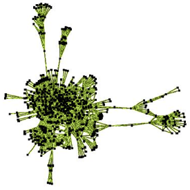
Figure 1: Representation of the medieval social network with force directed algorithm

As this is frequently the case, the obtained social network is a small-world network with low global connectivity and a high local connectivity [55, 54]. Indeed the diameter of $\mathcal{G}$ is $10$ and the mean of the shortest paths between two vertices is $3.9$. The local connectivity, measured by averaging the density of subgraphs induced by the direct neighbors of a vertex [54], is $77\%$ whereas the density of the graph is only $2.2\%$. The degree distribution also obeys to standards (see [15, 39, 34]): the cumulative degree distribution for the weighted graph fits a power-law with a fast decaying tail as shown in Figure 2. It follows that the number of vertices having a degree $k$ is decreasing very fast (exponentially) when $k$ increases and is not centered on a mean value: most of the peasants have a small number of relationships and a tiny number of them have numerous relationships.

Figure 2: Cumulative degree distribution (solid) of the weighted graph fitting $P(k)=1.12k^{-0.37}e^{-0.0009k}$ (dashed).

5.3 Clustering the medieval graph into perfect communities and rich-club

By the use of Theorem 1, all the perfect communities of a graph $\mathcal{G}$ can be computed. They emphasize the main dense parts of the social networks but also discriminate individuals by their relationships (direct neighbors). 76 perfect communities were found in $\mathcal{G}$, most of them being very small (only 2 or 3 persons).

Then, as described in Section 2, the rich-club and central vertices are extracted. The vertices in the rich club corresponds to the largest subgraph with highest degrees vertices having a diameter equal to 2. The rich club contains 3% of the vertices of the whole graph which corresponds to 19 vertices. This subgraph has a high density as shown in Figure 3.

Figure 3: Left: Density of the induced subgraph as a function of the number of highest degrees vertices (log scale) and Right: Number of components of the subgraph of perfect community and rich club as a function of the number of vertices with high betweenness measure added (in both cases, the number of vertices under consideration is given as a percentage of the total number of vertices in the graph).

Central vertices are chosen to be the 4% of the highest betweenness measure vertices of the whole graph (i.e., 24 vertices). As show in Figure 3, it is a good compromise for this application: the derived subgraph contains 8 components and a large number of vertices is needed to decrease this number again. Moreover, except for one of them, these components are tiny single perfect communities that won’t be considered in the following.

Figure 4 provides a representation of the perfect communities structure of the medieval social network together with the rich-club and central vertices. The visual representation of each perfect community has several features. The surface of each disk is proportional to the size of the perfect community (i.e., to the number of peasants in the perfect community) which is also recalled explicitly by a number written inside the circle. The gray level of the disk encode the mean date of the contracts in which the members of the community are involved (from black, 1260, to white, 1340). In addition a family name is added when the corresponding perfect community comes from a single family. The communities are set at random positions but efforts have been done to represent perfect communities that are linked by an edge at nearby positions. Two perfect communities that are linked by an edge form a complete subgraph but the peasants in this subgraph do not necessarily have the same outside relationships; on the contrary, two peasants contained in the same perfect community have exactly the same outside links. Links starting from a community are therefore valid for all the members of this community. Seven communities, that are still not connected with another perfect community, with the rich club or with one of the vertices with a high betweenness measure, were not considered for this representation.

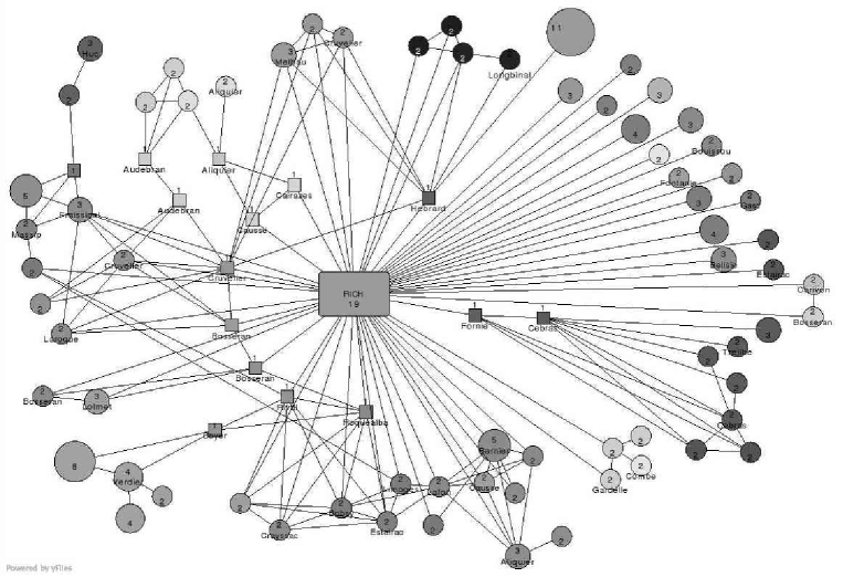
Figure 4: Graph of the perfect communities (circles), the rich-club (rectangle) and central vertices (squares). Other details about the figure are given in the text.

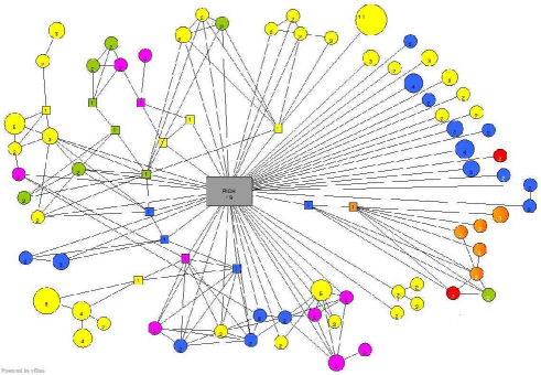
Figure 5: Graph of the perfect communities by geographical locations (yellow: Flaugnac, blue: Saint-Julien, green: Pern, pink: Cornus, red: Ganic and orange: Divilhac).

Figure 5 provides an alternative representation of the communities of the graph. Noting that the peasants of a perfect community lived at the same geographical location, each perfect community is colored to represent this location. The communities are set at the same positions as in Figure 4.

Of course, these representations have to be interpreted with care; some of their properties could induce interpretation biases. One of the main limitation is that only a part of the vertices of the original graph is represented on it (35 % of them). Moreover, the respective positions of the perfect communities can be relevant (if their are linked) or not (if they are not). Nevertheless, these “maps” of the graph allows to understand some important facts about the medieval society. First of all, the “small world” structure of the graph is emphasized by the star shaped structure of the perfect communities around the rich-club: some persons seem to belong to small groups (a perfect community or linked perfect communities) which are only related to each others by the way of the main individuals (the rich-club or peasants with a high betweenness measure).

Then, family links seem to have a great importance in the medieval society as all individuals in the perfect communities often share the same family name (this is the case for 30 perfect communities) but geographical proximities are even more important: as shown in Figure 5, all the perfect communities have homogeneous locations and very often, linked perfect communities also share the same geographical location. Finally, it appears that persons with a high degree of betweenness share the same geographical location as the perfect communities they are linked to. These individuals can be seen as peasants making the link between several villages or between a village and one of the central person from the rich-club.

5.4 Mapping the medieval graph with the SOM

The social network was analyzed with the batch kernel SOM as follows. The parameter $\beta$ varied between $0.01$ to $0.05$. Values above $0.05$ lead to instability in the calculation of the diffusion matrix in the sense that the obtained kernel is no more positive. Values smaller than $0.01$ lead to hard clustering (the diffusion matrix is close to the identity matrix) that are not relevant (see [52]).

For a fixed kernel (i.e., a value of $\beta$), all squared maps from $5\times 5$ to $10\times 10$ were tested as prior structures of the grid. For each prior structure, several random initial configurations, the kernel PCA based initial configuration and several initial temperatures were compared via Kaski and Lagus’ quality measure, leading to the selection of a single final map for each size (it should be noted that kernel PCA, associated to an optimal choice of the initial temperature, leads to much better results than random initialization).

In terms of $q$-modularity, the quality of clustering results increases with the value of $\beta$ (for almost all map sizes). As a consequence, the value of $\beta=0.05$ was selected. Among the 6 maps built with this kernel, those of size $6\times 6$ and $7\times 7$ are the most interesting. The first one has the highest $q$-modularity, whereas the second has the smallest value of $\mathcal{KL}$ criterion together with a high value of the $q$-modularity.

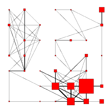
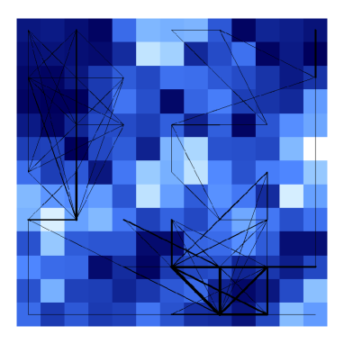
Figure 6: Final self-organizing map ($7\times 7$ square grid)

We decided to focus on the $7\times 7$ map as it seems to be the most interesting. It contains 35 non empty clusters and is given in the left part of Figure 6. In this graphical representation, the surface occupied by a square is proportional to the size of the corresponding cluster, while the width of the connection between two squares is proportional to the total weight of the edges connecting vertices of the two clusters.

The right part of Figure 6 is the U-matrix [48] of the map. It visualizes distances between prototypes (in the mapped space): dark colors correspond to close prototypes and light colors to a large distance between the corresponding prototypes.

The map is divided into three dense subparts: top-left, top-right and bottom-right. The number of edges is small between these three parts and much more dense inside the clusters of the same part, which seems to be relevant. The most dense part of the map is the bottom-right one: one of its clusters contains 255 vertices, which represents more than one third of the whole graph. This part is connected to the two others which are not connected to each others.

As the largest cluster still seems to be too large to be relevant, another batch kernel SOM was constructed on the subgraph induced by the vertices of this cluster; this methodology is known as a hierarchical feature maps [31]. As before a $7\times 7$ map is selected. It is represented in Figure 7.

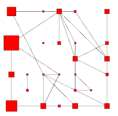
Figure 7: Self-organizing map of the main cluster

This map seems to be well connected except 3 little clusters that are not connected to the rest of the map. The final map is sparse and well organized. Once again, the main cluster of this map contains a high number of vertices, 81, which represents almost one third of the whole subgraph.

Such a phenomen reflects the cumulative degree distribution described in Section 5.2. An analysis of the degree distribution on the map of Figure 6 shows that the 10% of the vertices having the highest degrees are all clustered in three clusters of the bottom right part of the map (but not in the largest one, GC). Then, looking at the degrees of the subgraph made from the vertices in cluster GC, we see that, once again, their cumulative distribution is a power-law cumulative distribution but with another scale (the density of this subgraph is 5 times smaller than the one of the initial graph). The same phenomenon occurs in the subgraph GC: the 10% of the vertices that have the highest degrees are all assigned to the three mainly connected clusters of Figure 7 and the largest cluster of this subgraph (GC20) also has a density 4 times less than the whole subgraph GC.

5.5 Historical properties of the self-organizing map

The analysis mimics what has been done for the perfect communities, starting with the distribution of the dates on the map. The mean date for each cluster is depicted on Figure 8 using a gray scale. Each cluster has a small standard deviation; clusters having the highest standard deviations are the most connected clusters of the bottom right part of the map.

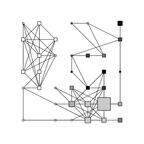
Figure 8: Mean date for each cluster from black, 1260, to white, 1340

The three parts of the Kohonen map emphasized by the U-matrix have homogeneous dates: top right is the oldest part, bottom right have middle dates and top left, the most recent dates. The clusters are continuously connected to each others by the date, in the sense that connexion clusters have intermediate dates. The organization provided by the SOM is therefore relevant. But, since the studied period is only 100 years long, this also seems to show that various generations (sons, fathers, grand-fathers,…) are not highly mixed; particularly, the earlier part of the map is only connected to the rest by a very few number of individuals (1 to 3).

The geographical locations of the persons belonging to the same cluster are generally homogeneous. More precisely, they are exactly the same for peasants belonging to the same little cluster and the largest clusters often have a dominant geographical location but also contain peasants that don’t live in this geographical location. The family names are generally not the same for peasants in the same cluster, with some exceptions as, for example, cluster 10 which corresponds to “Aliquier” family, just as one of its closest cluster, 11. Thus, as already mentioned in the analysis of the perfect communities, geographical proximities seem to have a main role in the peasant’s relationships.

5.6 Comparison with the work on perfect communities

A comparison of the self-organizing map with the perfect community representation (Figure 4) is provided by Figure 9: the vertices that belong to the same perfect community are almost always in the same cluster of the self-organizing maps (except for three small perfect communities). To study the reverse mapping, an arbitrary color was assigned to each cluster that contains at least one perfect community and then used to color the same way the perfect communities of Figure 4. The number assigned to each perfect community is the number of the cluster in one of the two maps (prefixed by “GC” for the clusters of the largest cluster of the initial SOM).

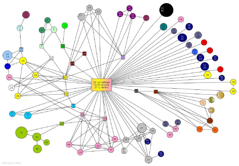
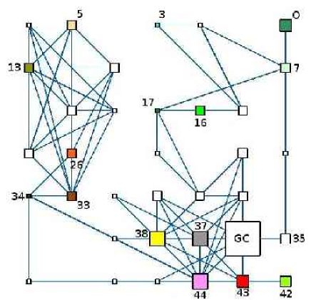
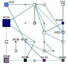
Figure 9: Comparison of the representation of the graph through perfect communities and self-organizing maps (left : of the whole graph; right : of the largest cluster of the initial SOM. More details about this figure are given in the text)

Figure 9 emphasizes the great similarity between the two approaches: perfect communities that share links often belong to the same cluster of the self organizing map. A similar remark can be made about peasants with a high betweenness measure: they are often assigned to the same cluster as the perfect community that they link to the rich-club. Moreover, perfect communities that share a link or that are linked to the same peasant with a high betweenness measure but have different colors often belong to nearby clusters on the SOM: this is the case, for example, for clusters 44 and 37, for clusters 0 and 7, for clusters 26, 33 and 34, etc. It is also interesting to note that some of the persons having a high betweenness measure also have an important position on the SOM: for example, peasants 17 and 34 are emphasized by the fact that they link the bottom right part of the map with the top right part and the top left part, respectively. All these similarities are evidence that there is a strong consensus between both approaches and, as a consequence, that they offer a realistic representation of the organization of the peasant society in the Middle Ages.

Nevertheless, there are also some interesting differences between the two approaches. First of all, it is suprising that the rich-club is separated in several clusters (37, 38 and 44) in which some perfect communities can also be found. Arguably, these three clusters are very close on the SOM and have strong connectivity (depicted by the tick lines between them). Moreover, the three clusters of the SOM correspond to different geographical locations: cluster 37 contains a majority of peasants living in “Cornus”, cluster 38 and 44 in “Saint Julien”. In addition, Clusters 38 and 44 also contains peasants that have different family names: “Belisie”, “Bernier”, “Bosseran”, “Cruvelier”, “Laroque”, “Ratier” and “Sirven” are found several times in cluster 38 but none in cluster 44 and “Amilhau”, “Camberan”, “Labarthe”, “Limoges”, “Rival” and “Tessendie” are found several times in cluster 44 but none in cluster 38. However, families “Estairac” and “Fague” are well represented in both clusters 38 and 44. It is therefore not very clear whether the separation of the rich-club into three clusters is relevant or not. An advantage of the rich-club approach over the SOM based analysis is to emphasize the members of this group who clearly have a special social role, while there is nothing very specific about the corresponding clusters in the map.

It appears also that some perfect communities share the same color whereas they don’t seem to be “close”. Sometimes, this is due to the fact that the positions of these perfect communities are partially random despite the fact they are linked to each others (this is the case, for instance, for the pink group of perfect communities 44 at the bottom of the figure and the perfect community of the same color at the left part of it). Sometimes, this can be explained by links that are not represented on the figure: for example, cluster 38 is separated into three groups of perfect communities that are not linked to each other but these groups share some common relationships with vertices in cluster 38 in the rich-club. However this argument is less convincing to explain why cluster 37 contains two groups of perfect communities. Finally, in some cases, there is no simple reason to explain why several perfect communities are grouped in the same cluster: for example, GC20 is still a large cluster that contains several perfect communities that are not linked to each others on the perfect communities representation.

5.7 Conclusion

The remarks made about the similarities and differences between the two approaches show that they can both provide elements to help the historians to understand the organization of the medieval society. Moreover, they have distinct advantages and weaknesses.

On the one hand, representing the graph through its perfect communities induces the question of the way these communities have to be represented in a two-dimensional space, even if the restrictive definition chosen for communities partly reduces this problem. This question is difficult (and related to the field of graph drawing) but of a great importance to avoid interpretation bias. For this point, the kernel SOM can appear as an alternative that provides a notion of proximity, organization and even distance between the communities. Moreover, kernel SOM allows to organize all the vertices of the graph and not only the vertices that belong to a perfect community.

On the other hand, the links inside and outside the clusters of the kernel SOM are not clear: some of the vertices in a cluster can have no edge in common with the other vertices of the cluster (it is the case, e.g., for one of the cluster of the largest cluster as is shown by Figure 7) and two vertices in the same cluster are not necessarily related to the same vertices outside the cluster. These two facts seem to show that kernel SOM probably provides a better macroscopic view of the graph, whereas the perfect community approach is more reliable for local interpretations: as the definition of a perfect community is restrictive, it emphasizes very close social groups that share the same geographical location and also often the same family name. The interpretation of such social groups is then easier.

It should be noted that in both cases, the social and historical analysis is only facilitated by the algorithms rather than somehow being automated. In a sense, the problem of understanding the social network is simply pushed a little bit further away by the methods, especially in the case of the kernel SOM. Figures 6 and 7 for instance give broad pictures of the social network, but a more detailed analysis is needed to extract knowledge from the network. One of the interesting aspect of the combined methodology proposed in the present paper is to help this detailed analysis.

To go further, an open question is the way the parameters of the kernel SOM have to be chosen and especially the size of the map, or, in the same spirit, how deep a hierarchical analysis should be conducted on a large cluster. This question is related to finding a relevant size for each community. The perfect community approach can help driving this work by providing an idea of the relevance of a given cluster, as we emphasized for cluster GC20.

Conversely, kernel SOM could also help to provide a more realistic representation of the perfect communities in creating a drawing algorithm that can also take into account the distances between clusters in the SOM. This question is currently under development.

6 Acknowledgments

The authors would like to thank Florent Hautefeuille, historian (FRAMESPA, Université Toulouse Le Mirail, France) for giving us the opportunity to work with this interesting database and for spending time to explain us its historical context. We also want to thank Fabien Picarougne and Bleuenn Le Goffic (LINA, Polytech’Nantes, France) for managing the database registration and Pascale Kuntz for her expertise in graph vizualisation. We finally thank the anonymous reviewers for their detailed and constructive comments that have significantly improved this paper.

References

- [1] C. Alpert, A. Kahng, Geometric embeddings for faster and better multi-way netlist partitioning, in: Proceedings of the 30th International Conference on Design Automation (DAC ’93), ACM Press, New York, USA, 1993.
- [2] C. Ambroise, G. Govaert, Analyzing dissimilarity matrices via Kohonen maps, in: Proceedings of 5th Conference of the International Federation of Classification Societies (IFCS 1996), vol. 2, Kobe (Japan), 1996.
- [3] P. Andras, Kernel-Kohonen networks, International Journal of Neural Systems 12 (2002) 117–135.
- [4] N. Aronszajn, Theory of reproducing kernels, Transactions of the American Mathematical Society 68 (3) (1950) 337–404.
- [5] D. Auber, Tulip : A huge graph visualisation framework, in: P. Mutzel, M. Jünger (eds.), Graph Drawing Softwares, Mathematics and Visualization, Springer-Verlag, 2003, pp. 105–126.
- [6] A. Berlinet, C. Thomas-Agnan, Reproducing Kernel Hilbert Spaces in Probability and Statistics, Kluwer Academic Publisher, 2004.
- [7] S. Bornholdt, H. Schuster, Handbook of Graphs and Networks - From the Genome to the Internet, Wiley-VCH, Berlin, 2002.
- [8] F. Chung, Spectral Graph Theory, No. 92 in CBMS Regional Conference Series in Mathematics, American Mathematical Society, 1997.
- [9] A. Clauset, M. E. J. Newman, C. Moore, Finding community structure in very large networks, Physical Review, E 70 (2004) 066111.
- [10] B. Conan-Guez, F. Rossi, A. El Golli, Fast algorithm and implementation of dissimilarity self-organizing maps, Neural Networks 19 (6-7) (2006) 855–863.
- [11] N. Cristianini, J. Shawe-Taylor, J. Kandola, Spectral kernel methods for clustering, in: T. Dietterich, S. Becker, Z. Ghahramani (eds.), Advances in Neural Information Processing Systems (NIPS), vol. 13, MIT Press, Cambridge, MA, 2001.
- [12] G. Di Battista, P. Eades, R. Tamassia, I. Tollis, Graph Drawing, Prentice Hall, Upper Saddle River, NJ, USA, 1999.
- [13] L. Donetti, M. Muñoz, Detecting network communities: a new systematic and efficient algorithm, Journal of Statistical Mechanics: Theory and Experiment (2004) P10012.
- [14] A. El Golli, F. Rossi, B. Conan-Guez, Y. Lechevallier, Une adaptation des cartes auto-organisatrices pour des données décrites par un tableau de dissimilarités, Revue de Statistique Appliquée LIV (3) (2006) 33–64.
- [15] M. Faloutsos, P. Faloutsos, C. Faloutsos, On power-law relationships of the internet topology, ACM SIGCOMM Computer Communication Review 29 (4) (1999) 251–262.
- [16] M. Filippone, F. Camastra, F. Masulli, S. Rovetta, A survey of kernel and spectral methods for clustering, Pattern Recognition 41 (2008) 176–190.
- [17] T. Graepel, M. Burger, K. Obermayer, Self-organizing maps: generalizations and new optimization techniques, Neurocomputing 21 (1998) 173–190.
- [18] T. Graepel, K. Obermayer, A stochastic self-organizing map for proximity data, Neural Computation 11 (1) (1999) 139–155.
- [19] B. Hammer, A. Hasenfuss, Relational topographic maps, Tech. Rep. IfI-07-01, Clausthal University of Technology, avaliable at http://www.in.tu-clausthal.de/fileadmin/homes/techreports/ifi0701hammer%.pdf (2007).
- [20] B. Hammer, A. Hasenfuss, M. Rossi, F. annd Strickert, Topographic processing of relational data, in: Proceedings of the 6th Workshop on Self-Organizing Maps (WSOM 07), Bielefeld, Germany, 2007, to be published.
- [21] B. Hammer, A. Micheli, M. Strickert, A. Sperduti, A general framework for unsupervised processing of structured data, Neurocomputing 57 (2004) 3–35.
- [22] F. Hautefeuille, Structures de l’habitat rural et territoires paroissiaux en bas-Quercy et haut-Toulousain du VIIème au XIVème siècle, Ph.D. thesis, University of Toulouse II (Le Mirail) (1998).
- [23] I. Herman, G. Melançon, M. Scott Marshall, Graph visualization and navigation in information visualisation, IEEE Transactions on Visualization and Computer Graphics 6 (1) (2000) 24–43.
- [24] S. Kaski, K. Lagus, Comparing self-organizing maps, in: C. von der Malsburg, W. von Seelen, J. Vorbrüggen, B. Sendhoff (eds.), Proceedings of International Conference on Artificial Neural Networks (ICANN’96), vol. 1112 of Lecture Notes in Computer Science, Springer, Berlin, Germany,, 1996, pp. 809–814.
- [25] T. Kohohen, P. Somervuo, Self-Organizing maps of symbol strings, Neurocomputing 21 (1998) 19–30.
- [26] T. Kohonen, Self-organizing maps of symbol strings, Technical report a42, Laboratory of computer and information science, Helsinki University of technoligy, Finland (1996).
- [27] T. Kohonen, Self-Organizing Maps, 3rd Edition, vol. 30, Springer, Berlin, Heidelberg, New York, 2001.
- [28] T. Kohonen, P. Somervuo, How to make large self-organizing maps for nonvectorial data, Neural Networks 15 (8) (2002) 945–952.
- [29] R. Kondor, J. Lafferty, Diffusion kernels on graphs and other discrete structures, in: Proceedings of the 19 International Conference on Machine Learning, 2002.
- [30] D. Mac Donald, C. Fyfe, The kernel self organising map., in: Proceedings of 4th International Conference on knowledge-based intelligence engineering systems and applied technologies, 2000.
- [31] R. Miikkulainen, Script recognition with hierarchical feature maps, Connection Science 2 (1990) 83–101.
- [32] B. Mohar, The laplacian spectrum of graphs, vol. 2, chap. Graph Theory, Combinatorics, and Applications, Wiley, 1991, pp. 871–898.
- [33] B. Mohar, S. Poljak, Eigenvalues in combinatorial optimization, vol. 50 of IMA Volumes in Mathematics and Its Applications, chap. Combinatorial and Graph-Theoretical Problems in Linear Algebra, Springer-Verlag, 1993, pp. 107–151.
- [34] S. Mossa, M. Barthélémy, H. Stanley, L. Nunes Amaral, Truncation of power law behavior in “scale-free” network models due to information filtering, Physical Review Letters 88 (13) (2002) 138701.
- [35] J. Neville, M. Adler, D. Jensen, Clustering relational data using attribute and link information, in: Proceedings of the Text Mining and Link Analysis Workshop, 18th International Joint Conference on Artificial Intelligence, 2003.
- [36] M. Newman, Mixing patterns in networks, Physical Review, E 67 (2003) 026126.
- [37] M. Newman, A. Barabási, D. Watts, The Structure and Dynamics of Networks, Princeton University Press, 2006.
- [38] M. Newman, M. Girvan, Finding and evaluating community structure in networks, Physical Review, E 69 (2004) 026113.
- [39] M. Newman, D. Watts, S. Strogatz, Random graph models of social networks, Proceedings of the National Academy of Sciences of the United States of America 99 (2002) 2566–2572.
- [40] G. Palla, I. Derenyi, I. Farkas, T. Vicsek, Uncovering the overlapping community structure of complex networks in nature and society, Nature 435 (7043) (2005) 814–821.
- [41] P. Pons, M. Latapy, Computing communities in large networks using random walks, Journal of Graph Algorithms and Applications 10 (2) (2006) 191–218.
- [42] F. Radicchi, C. Castellano, F. Cecconi, V. Loreto, D. Parisi, Defining and identifying communities in networks, Proceedings of the National Academy of Sciences of the United States of America 101 (2004) 2658–2663.
- [43] S. Schaeffer, Graph clustering, Computer Science Review 1 (1) (2007) 27–64.
- [44] B. Schölkopf, A. Smola, K. Müller, Nonlinear component analysis as a kernel eigenvalue problem, Neural Computation 10 (1998) 1299–1319.
- [45] B. Schölkopf, K. Tsuda, J. Vert, Kernel methods in computational biology, MIT Press, London, 2004.
- [46] A. Smola, R. Kondor, Kernels and regularization on graphs, in: M. Warmuth, B. Schölkopf (eds.), Proceedings of the Conference on Learning Theory (COLT) and Kernel Workshop, 2003.
- [47] S. Strogatz, Exploring complex networks, Nature 410 (2001) 268–276.
- [48] A. Ultsch, H. P. Siemon, Kohonen’s self organizing feature maps for exploratory data analysis, in: Proceedings of International Neural Network Conference (INNC’90), 1990.
- [49] J. van den Heuvel, S. Pejic, Using Laplacian eigenvalues and eigenvectors in the analysis of frequency assignment problems, Annals of Operations Research 107 (1-4) (2001) 349–368.
- [50] J. Vert, M. Kanehisa, Extracting active pathways from gene expression data, Bioinformatics 19 (2003) 238ii–244ii.
- [51] N. Villa, R. Boulet, Clustering a medieval social network by SOM using a kernel based distance measure., in: M. Verleysen (ed.), Proceedings of ESANN 2007, Bruges, Belgium, 2007.
- [52] N. Villa, F. Rossi, A comparison between dissimilarity SOM and kernel SOM for clustering the vertices of a graph, in: Proceedings of the 6th Workshop on Self-Organizing Maps (WSOM 07), Bielefield, Germany, 2007, to be published.
- [53] U. von Luxburg, A tutorial on spectral clustering, Tech. Rep. TR-149, Max Planck Institut für biologische Kybernetik, avaliable at http://www.kyb.mpg.de/publications/attachments/luxburg06_TR_v2_4139\%5B\%1\%5D.pdf (2007).
- [54] D. Watts, Small Worlds - The Dynamics of Networks between Order and Randomness, Princeton University Press, Princeton, New Jersey, 1999.
- [55] D. Watts, S. Strogatz, Collective dynamics of “small-world” networks, Nature 393 (1998) 440–442.
- [56] S. Zhou, R. Mondragon, The rich-club phenomenon in the Internet topology, IEEE Communications Letters 8 (3) (2004) 180–182.