Long-term temporal dependence of droplets transiting through a fixed spatial point in gas-liquid two-phase turbulent jets

Abstract

We perform rescaled range analysis upon the signals measured by Dual Particle Dynamical Analyzer in gas-liquid two-phase turbulent jets. A novel rescaled range analysis is proposed to investigate these unevenly sampled signals. The Hurst exponents of velocity and other passive scalars in the bulk of spray are obtained to be 0.59$\pm$0.02 and the fractal dimension is hence 1.41$\pm$ 0.02, which are in remarkable agreement with and much more precise than previous results. These scaling exponents are found to be independent of the configuration and dimensions of the nozzle and the fluid flows. Therefore, such type of systems form a universality class with invariant scaling properties.

, , , , ,

1 Introduction

It is well known that Richardson-1922 ’s picture of turbulent cascade, in which large eddies break down into smaller ones, is a multiplicative process. This hierarchical cascade in turbulence can be described by fractal geometry Mandelbrot-1974-JFM , which is characterized quantitatively by the fractal dimension of self-similar structure of turbulence Mandelbrot-1983 , Frisch-1996 . Both the experimental and theoretical aspects have been studied in past decades.

Lovejoy investigated the fractal nature of satellite- and radar-determined cloud and rain areas covering 6 orders of magnitude of area sizes Lovejoy-1982-Science . The area-perimeter relation, introduced by Mandelbrot Mandelbrot-1983 , was found to hold with the fractal dimension $D_{1}=1.35\pm 0.05$. A theoretical analysis was proposed by Hentschel and Procaccia Hentschel-Procaccia-1984-PRA . They developed a theory of turbulent diffusion and obtained the natural consequence that $1.37<D_{1}<1.41$, which is in excellent agreement with the empirical results of Lovejoy Lovejoy-1982-Science .

Another important experiment concerns the studies on the fractal facet of the turbulent-nonturbulent interface in turbulent flows by Sreenivasan and his coworkers Sreenivasan-Meneveau-1986-JFM , Sreenivasan-Ramshankar-Meneveau-1989-PRSA , Prasad-Sreenivasan-1990-PFA . Prasad and Sreenivasan applied the laser-induced fluorescence technique to obtain the images of two-dimensional cuts of turbulent jets Prasad-Sreenivasan-1989-EF , Prasad-Sreenivasan-1990-JFM . Applying the box-counting method, they estimated the fractal dimension of turbulence interface in the K range and found that $D_{2}=2.36\pm 0.05$ for all fully turbulent flows Prasad-Sreenivasan-1990-PFA . Taking into account the influence of local fluctuations in the Kolmogorov scale on the surface area due to the multifractal nature of the rate of dissipation, slight revision was made Meneveau-Sreenivasan-1990-PRA . In addition, Huang et al. proposed a modified box-counting method and found that $D_{2}=2.43\pm 0.04$ in the K range for round jets Huang-Li-Yu-1994-CSB .

All the above experimental results are based on the box-counting method, which may lead to several disadvantages and difficulties. Difficulties associated with box-methods are typically attributed to the lack of a significant scaling range, low signal-to-noise ratio that limits reliable determination of level sets, and possible inadequate records resulting in poor statistics confidence. Several methods proposed to analyze box-counting statistics that do not presume power-law behaviors have been employed to address the first issue, which aim at determining the scaling range, if any, in an unbiased fashion. In addition, the linear correlation coefficient in log-log plots is not high enough, which results in relatively large standard deviations. It is well know that, for fractals with underlying cascade process, there are logarithmic periodic oscillations Badii-Politi-1984-PLA , Smith-Fournier-Spiegel-1986-PLA , Sornette-1998-PR , Johansen-Sornette-Hansen-2000-PD , Zhou-Sornette-2002-PD , Zhou-Sornette-Pisarenko-2003-IJMPC . The logarithmic periodic oscillations can be used to explain why different samplings lead to different estimates of fractal dimension. Zhou and Sornette proposed that canonical averaging of variety of samplings can be used to eliminate logarithmic periodic oscillations and get more reliable fractal dimension Zhou-Sornette-2002-PD .

Alternatively, rather than using the classic box-counting method, Zhou et al. performed a rescaled range analysis upon signals measured by Dual PDA to determine the fractal dimension of coaxial turbulent jet, in which one-dimensional cuts are handled and the unequally spaced time series were pre-processed using averaging to form equidistantly spaced series Zhou-Wu-Zhao-Yu-2000-HGXB . The fractal dimension was found to be $D_{1}=1.42\pm 0.07$. Since the rescaled range analysis is conducted based on averaging different subseries at each scale, possible log-periodic oscillations are eliminated. However, the moving averaging interpolation approach is not satisfying. In this paper, we shall develop a variant of the rescaled range analysis to make it suit directly for unequally spaced time series such that the corresponding results are more precise.

This paper is organized as follows. In Sec. 2, we propose a generalization of the classical rescaled range analysis. Section 3 reports the experiential results and corresponding fractal dimensions for a variety of experiments under different conditions. By comparing with interface dimensions of scalar field, physical interpretation is presented in Sec. 4. Section 5 concludes.

2 Rescaled range analysis

Rescaled range analysis, also termed as $R/S$ analysis or Hurst analysis, was originally developed by Hurst Hurst-1951-TASCE . This analysis is based on a new statistical development and provides an approach for analysis and characterization of time series which has no underlying periodicity, yet retains long term correlation Mandelbrot-Wallis-1969a-WRR , Mandelbrot-Wallis-1969b-WRR , Mandelbrot-Wallis-1969c-WRR , Mandelbrot-Wallis-1969d-WRR . The classic $R/S$ analysis is performed on a discrete time series data set $\left\{y_{i}:i=1,2,\cdots,n\right\}$ with the time $t_{i}$ uniformly-spaced, which is however not suitable for other time series that are not equidistantly sampled, such as data measured by Dual PDA. We thus generalize the classic $R/S$ analysis from equidistant sampling to uneven sampling.

Define a continuous function $y:\left[a,b\right]\rightarrow\Re$. In a certain sense, graph

$$graph\left(y\right)=\left\{\left(t,y\left(t\right)\right):t\in\left[a,b\right]\right\}$$ (1)

may be regarded as a 2-dimensional fractal in the plane $\left(t,y\right)$. Falconer has presented a method to estimate the fractal dimension of functional graph Falconer-2003 . Let $\left[\tau_{1},\tau_{2}\right]\subset\left[a,b\right]$. The time span $s=\tau_{2}-\tau_{1}$ of $y$ is referred to as “lag” Mandelbrot-Wallis-1969b-WRR , Mandelbrot-Wallis-1969c-WRR . Then the mean of $y$ on $\left[\tau_{1},\tau_{2}\right]$ is

$$\left\langle y\right\rangle=\frac{1}{\tau_{2}-\tau_{1}}\int\nolimits_{\tau_{1}}^{\tau_{2}}y\left(t\right)\rm{d}t.$$ (2)

Define the cumulative deviation to be

$$X\left(t\right)=\int\nolimits_{\tau_{1}}^{t}\left[y\left(t\right)-\left\langle y\right\rangle\right]\rm{d}t$$ (3)

and the cumulative range to be

$$R=\underset{\tau_{2}\geqslant t\geqslant\tau_{1}}{\sup}X\left(t\right)-\underset{\tau_{2}\geqslant t\geqslant\tau_{1}}{\inf}X\left(t\right).$$ (4)

The standard deviation is

$$S=\left\{\frac{1}{\tau_{2}-\tau_{1}}\int\nolimits_{\tau_{1}}^{t}\left[y\left(t\right)-\left\langle y\right\rangle\right]^{2}\rm{d}t\right\}^{\frac{1}{2}}.$$ (5)

Therefore, as a generalization of the $R/S$ analysis for discrete time series, we assume that ${R}/{S}$ is self-affine and scales with respect to $s$ as a power law

$${R}/{S}\varpropto\left(\tau_{2}-\tau_{1}\right)^{H}=s^{H},$$ (6)

where $H$ is termed as the Hurst exponent.

Partition the interval $\left[\tau_{1},\tau_{2}\right]$ into $n$ divisions with $\tau_{1}=t_{0}<t_{1}<\cdots<t_{n}=\tau_{2}$. Then $y_{i}=y\left(t_{i}\right)$ is a unequally spaced time series. Using rectangular approximation for integration, one can descretize Eqs. (2)-(6) as follows.The mean of $y$ can be regarded as a time-weighted average

$$\left\langle y\right\rangle=\frac{1}{t_{n}-t_{0}}\overset{n}{\underset{i=1}{\sum}}y_{i}\times\left(t_{i}-t_{i-1}\right),$$ (7)

and the cumulative range becomes

$$R=\underset{1\leqslant j\leqslant n}{\max}\left\{X_{j}\right\}-\underset{1\leqslant j\leqslant n}{\min}\left\{X_{j}\right\},$$ (8)

where

$$X_{j}=\overset{j}{\underset{i=1}{\sum}}\left(y_{i}-\left\langle y\right\rangle\right)\left(t_{i}-t_{i-1}\right)$$ (9)

is the cumulative deviation. Taking into account the weighted standard deviation

$$S=\left\{\frac{1}{t_{n}-t_{0}}\overset{n}{\underset{i=1}{\sum}}\left(y_{i}-\left\langle y\right\rangle\right)^{2}\left(t_{i}-t_{i-1}\right)\right\}^{\frac{1}{2}},$$ (10)

we have

$${R}/{S}\varpropto\left(t_{n}-t_{0}\right)^{H}=s^{H}.$$ (11)

If $t_{i}-t_{i-1}=\Delta t$ is a constant, the cumulative deviation $X_{j}$ given in (9) is $\Delta t$ times that in the conventional $R/S$ analysis for uniformly spaced time series data. However, it has no impact on the estimation of Hurst exponent using Eq. (11). The Hurst exponent $H$ of the time series is then evaluated from the slope of the straight line fitted to these points. The estimated Hurst exponent is related to its fractal dimension $D$ by the relation Mandelbrot-1983

$$D=2-H.$$ (12)

The $R/S$ analysis is a simple and robust method for fast fractal estimate with as few as 30 data points Handley-Jaenisch-Bjork-Richardson-Carruth-1993-Simulation .

There are a variety of algorithms for performing $R/S$ analysis. Consider a subseries $\left\{y_{i},y_{i+1},\cdots,y_{i+s-1}\right\}$, where $i$ is the departure of the sub-series and $s$ is the length of the sub-series with $1\leqslant i<i+s-1\leqslant n$. Different selection of $i$ and $s$ results in different algorithm. In this paper, we propose to adopt a random selection algorithm, in which $m$ starting points $i$ are chosen randomly based on a uniform distribution on the interval $[1,n-s+1]$. An average of the $m$ values of $R/S$ with the same lag $s$ is calculated, which is denoted by ${R\left(s\right)}/{S\left(s\right)}$. The Hurst exponent can be calculated according to Eq. (11).

3 Experimental measurement of fractal dimensions

3.1 Experimental set-up

The Dual PDA is based on a novel concept that yields a higher measurement accuracy and performs non-intrusive measurements of the velocity, diameter and transit time of spherical particles, droplets and bubbles suspended in gaseous or liquid flows, particularly for spray analysis and other investigations of liquid atomization. The underlying principle of phase Doppler anemometry is based on light-scattering interferometry and therefore requires no calibration. The measurement point is defined by the intersection of two or three pairs of focused laser beams and the measurements are performed on single particles as they move through the measurement volume. Particles thereby scatter light from the laser beams, generating an optical interference pattern. A receiving optics placed at a well-chosen off-axis location projects a portion of the scattered light onto multiple detectors. Each detector converts the optical signal into a Doppler burst with a frequency linearly proportional to the particle velocity. The phase shift between the Doppler signals from different detectors is a direct measure of the particle diameter. We can obtain the arrival time and transit time simultaneously.

The Dual PDA receiving probe contains four receiving apertures integrated into one single optical unit. The Dual PDA detector configuration (2 standard and 2 planar), combined with sophisticated validation routines, is not susceptible to unwanted effects resulting from the Gaussian light intensity distribution in the measurement volume. Misinterpreted size measurements due to trajectory effects are therefore eliminated. The front optics module for 3D-PDA configurations simplifies the alignment procedure considerably. Screwed onto the PDA receiving probe and connected to the transmitter optics by a dual-fibre link, the front optics module generates the third pair of laser beams with adjustable beam intersection and focus. The received signals are fed to one of Dantec’s advanced signal processors, which delivers results to a PC. The instrument chart of the Dual PDA system is shown in Fig. 1. The power of the laser generator is 2W. The focal length of the transmitting and receiving lenses are both 500mm.

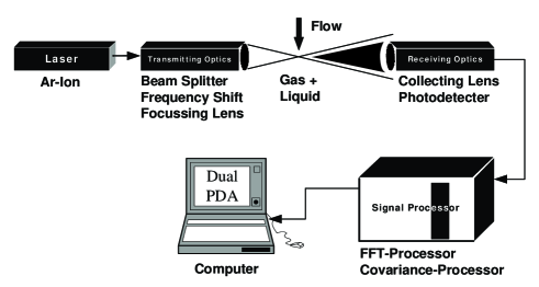
Figure 1: Experimental set-up of the Dual PDA system

3.2 Experimental conditions

In the experiments, we used tri-passage coaxial nozzles. The liquid phase water moves through the mid-passage, while the gaseous phase, say air, N₂ and CO₂, passes through the inner and outer passages. In the experiments, the gaseous medium is changeable and the fluid flow rates of the two phases are adjustable. The measurement points distribute through out the spray zone. For a fixed experimental configuration and given fluid flow, we record the arrival time $t$, transit time $T$, axial velocity $U$, radial velocity $V$ and drop diameter $d$ of 20000 drops moving through the measurement point. In experiment (a), the flows of nitrogen in the inner and outer passages are respectively 0.5 and 3.0m³/h, while those in the experiment (b) are $0.69$ and $3.9$m³/h, respectively.

For a fixed measurement point at $\left(0,0,-26\right)$, the data rate is $20.8$KHz, the mean velocity is $33.81$m/s, and the r.m.s. velocity is $9.51$ m/s. The Kolmogorov microscale $\eta$ is calculated from the signals according to

$$\eta=\left[\frac{\nu^{2}U_{1}^{2}}{15\left\langle\left(\partial U/\partial t\right)^{2}\right\rangle}\right]^{1/4}~{},$$ (13)

where $U_{1}$ is the mean speed at the measurement point, $\nu$ is the kinematic viscosity of air, and $U$ is the streamwise component of velocity. The resulting value of $\eta$ is $0.013$cm. The Taylor microscale $\lambda=0.41$cm is calculated according to

$$\lambda=\frac{U^{\prime}U_{1}}{\left\langle\left(\partial U/\partial t\right)^{2}\right\rangle^{1/2}}~{},$$ (14)

where $U^{{}^{\prime}}$ is the r.m.s. of velocity fluctuations. Hence, the Taylor-scale Reynolds number is

$${\rm{Re}}_{\lambda}=U_{1}\lambda/\nu=273~{},$$ (15)

which is moderate.

The power spectrum of the velocity signal is shown in Fig. 2 which is obtained by the Dual PDA Processor using the Gabor Fourier transform. A power-law scaling $E(k)\thicksim k^{-\beta}$ with an exponent $\beta$ close to $5/3$ is observed over a substantial range of about $0.7$ decades. Since the sampling frequencies are not high enough, the highest frequency is in the inertial range, which implies that we are dealing with the K-range in this work.

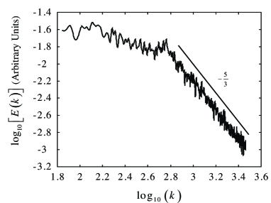
Figure 2: Energy spectrum of velocity signals

3.3 Hurst exponents and fractal dimensions

First of all, we analyzed the velocity signals arising from experiments by random selection algorithm. A typical diagram of $\ln(R/S)$ versus $\ln(s)$ is shown in Fig. 3. There is a transient regime for $\ln(s)<-6$, which exhibits a clear dropdown compared with the scaling regime. The slope of the trend line in the scaling regime gives the Hurst exponent $H=0.5926$. When adopting the approximation that the measurement is evenly spaced, the Hurst exponent estimated in the same scaling range is $\hat{H}=0.5518$, which is significantly smaller than the real value of $H$. This phenomenon is systematically observed for other experimental realizations.

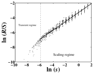
Figure 3: A typical diagram of $\ln(R/S)$ versus $\ln(s)$

According to the trend of Hurst exponents from the experiments, we can roughly classify the turbulent spray zone into two parts: the transient region and the steady region. In addition, the span of the transient zone is found to be proportional to the spray speed. Two typical diagrams of variation of Hurst exponent along the axial direction are shown in Fig. 4. It is obvious that there exists transient region near the outlet of the nozzle. The span of transient zone of (a) is about $2\sim 3$mm, while that of (b) is about $3\sim 4$mm. One can see that $H$ decreases along the streamwise direction near the outlet of the nozzle, which shows that the signals close to the nozzle have stronger persistency. This is induced by the stronger interactions among drops moving through the measurement points. After a short transient period, the four types of $H$ arrive a “steady” state, which fluctuates somewhat randomly near the average $0.59$. We should point out that the measurement range in the experiment with a distance from the outlet of the nozzle of about $200$mm is much wider than what we have presented in Fig. 4.

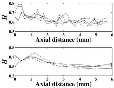
Figure 4: Typical diagrams of Hurst exponent evolution along axial direction

The Hurst exponents of axial and radial velocities are plotted in Fig. 5. The experiment conditions and/or the spatial position of measurement are different to each other. The hurst exponent is independent of experiment condition and the spatial position. It is easy to find that, there are several points with relatively higher $H$ of the axial velocity. These signals are nonstationary and are not available for $R/S$ analysis, which will be addressed later. Thus we withdraw these points. It follows that

$$H_{\rm{U}}=0.60\pm 0.02$$ (16)

and

$$H_{\rm{V}}=0.59\pm 0.02.$$ (17)

In fact, the existence of nonstationary signals does not affect the mean values, but they will increase the standard deviations.

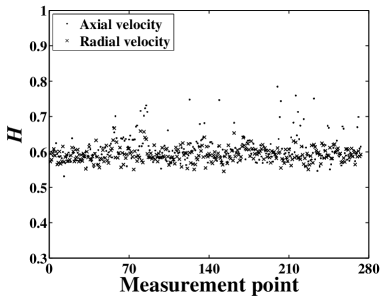
Figure 5: Hurst exponents of velocity signals

Similarly, the Hurst exponents of transit times and drop diameters are shown in Fig. 6. Nonstationary signals, especially of transit time, appear again. One can also find that, when investigating a signal with high $H$ in Fig.6, those signals from the same measurement record of the investigated signal have high $H$ as well. Withdrawal of these nonstationary signals follows that

$$H_{\rm{T}}=0.60\pm 0.02$$ (18)

and

$$H_{\rm{d}}=0.59\pm 0.02~{}.$$ (19)

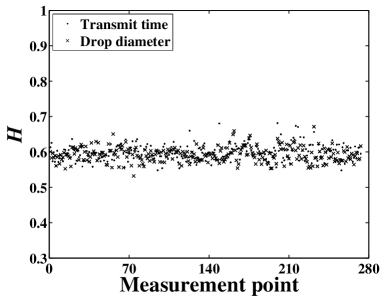
Figure 6: Hurst exponents of transit time and drop diameter signals

It is obvious that the Hurst exponents of different signals are identical to each other. The difference among the four types of $H$ is within the scope of experiment error. Consequently, the considered signals are also self-affine among each other. The histogram of the Hurst exponent distribution of all signals is shown in Fig. 7. The majority of Hurst exponents concentrate around the mean value $0.59$. The averaged Hurst exponent can thus be calculated as

$$H=0.59\pm 0.02~{}.$$ (20)

We can hence obtain the fractal dimension of the signals that

$$D=1.41\pm 0.02~{}.$$ (21)

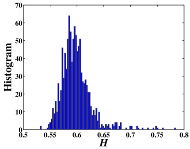
Figure 7: Histogram of Hurst exponents of all signals

In a nutshell, the Hurst exponent and the corresponding fractal dimension of the signals are independent of the spatial position of the measurement position. That is, the investigated turbulent jet is fractally homogenous in the main bulk of the spray zone. Moreover, we can say that such two-phase flows form a universal class with a universal Hurst exponent, since the fractal dimensions are invariant with the changes of nozzle configuration, fluid medium, and flow rates as well Zhou-Wu-Zhao-Yu-2000-HGXB . However, we should point out that the Hurst exponents change for other type of two-phase flows. For example, coherent structure appears when measuring signals of hydrogen jet into air Liu-Wu-Wang-Gong-Yu-2000-HGXB , Liu-Zhao-Wang-Gong-Yu-2000-HGXB . Such a self-organized structure is expected to strengthen the long-term dependence and decrease the fractal dimensions.

4 Discussions

4.1 Nonstationary signals

One may take it for granted that the computed Hurst exponent of a fixed record is not reproducible when a repeated calculation is carried out. However, we would like to point out the stability and repeatability of the random sub-series algorithm, which has been verified by repeating computations such that the resulting Hurst exponents change very slightly compared with the previously calculated values. Thus, it seems that the surprising high values of Hurst exponents in Fig. 5 and Fig. 6 are unavoidable. Fortunately, we found that signals corresponding to “unexpected” high values of $H$ are nonstationary which can be used to distinguish these signals from the rest. This is why we have got rid of experimental points with high $H$.

A random process, say the axial velocity $U(t)$, is called stationary if identical rules generate the process $U(t)$ itself and all the processes deduced from $U(t)$ by a time shift, namely, all the processes of the form $U(t+s)$. In experiments, we have to control the conditions to be fixed through out the measurement of one signal. Consequently, the mean of axial velocity component, denoted as $\left\langle U\left(s\right)\right\rangle$ where the averaging is performed over the time and $s$ is the sub-series length, must be a constant. For nonstationary signals in the experiments, an obvious change of $\left\langle U\left(s\right)\right\rangle$ is detected in the plot of $\left\langle U\left(s\right)\right\rangle$ against arrival time. In the present case, the nonstationary signal can be regarded as a patchwork of several stationary ones with different means. We find that, such a scrambling leads to an upward in the tail of large lag $s$, namely, the resulting Hurst exponent becomes higher. From a mathematical point of view, $\left\langle\frac{R\left(t,s\right)}{S\left(t,s\right)}\right\rangle$ for these nonstationary signals is dependent of $t$ and thus $R/S$ analysis is not applicable Mandelbrot-Wallis-1969d-WRR .

It is the usual situation that the flow flux decreases or increase suddenly. Therefore, in order to verify the validity of the claim, we performed numerical computations upon artificial series $u\left(t_{i}\right)$ which are generated using

$$u\left(t_{i}\right)=\left\{\begin{array}[]{lccl}U\left(t_{i}\right),&{}{}\hfil&{\rm{if}}&1\leqslant i\leqslant 10000\\ U\left(t_{i}\right)+\Delta u,&{}{}\hfil&{\rm{if}}&10001\leqslant i\leqslant 20000\end{array}\right.$$ (22)

from the real series $U\left(t_{i}\right)$, where $\Delta u$ is an adjustable non-zero parameter. Denote $H^{a}$ for the Hurst exponents of the artificial series. We find that $H^{a}\left(\Delta u\right)$ is approximatively equal to $H^{a}\left(-\Delta u\right)$ in a statistical sense, and $H^{a}$ increases with increasing $\left|\Delta u\right|$ in the sampling time intervals for all series. We use the same signal analyzed in Fig. 3 to show the effect of non stead by comparing the results of raw signal with manipulated signals ($\Delta{u}\neq 0$). For the sake of better presentation, we treat all the signals as evenly spaced. The results are shown in Fig. 8. The circles represent the real series, while the squares and pluses correspond to $\Delta u=10$ and $\Delta u=-10$, respectively. The solid line is used to guide the eyes. We can see that the real series has scaling behavior over the whole sampling interval. Nevertheless, the artificial series have a more narrow scaling range and an upward end, which results in the increase of the Hurst exponent.

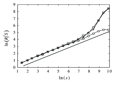
Figure 8: Comparison of rescaled range analysis on the real time series ($\circ$) and manipulated signals with $\Delta{u}=10$ ($\small\square$) and $\Delta{u}=-10$ ($+$)

Imagine a sudden drop in the flux of nitrogen in the outer passage such that $\left\langle U(s)\right\rangle$ decreases. $\left\langle T(s)\right\rangle$ will increase considerably due to the strong dependence of transit time on the axial velocity, while $\left\langle d(s)\right\rangle$ and $\left\langle V(s)\right\rangle$ increases slightly. These changes result in the in-step increases of $H$.

4.2 Comparison with interface dimension

It is natural to think that the passive scalars, the transit time and drop size, are strongly affected by the turbulent velocity field. Since the passive scalars are dependent of the turbulent field, the fluctuation of passive scalars shows the situation of turbulent field. If the investigated carriers are dense enough such that they form a continuous turbulent-nonturbulent interface, we can conjecture that the fractal dimension of the turbulent-nonturbulent interface depend strongly upon the fluctuation of the velocity and the passive scalars. We will find that the fractal dimensions of interfaces and signals are essentially identical.

It is obvious that, if the drops in the spray zone is dense enough, the spray can be regarded as a “cloud”. Furthermore, if the disperse phase in the spray aggregates to form larger bulk, interfaces appear. Such crossovers illustrate the intrinsic relationship among these systems. It is convenient to assume that there are local imaginary interfaces in the investigated system. It is well known that the area $S$ of the fractal interface can be expressed as Mandelbrot-1983

$$S\sim\eta^{2-D_{2}}.$$ (23)

We write $C$ for a scalar difference characteristic of large scales, such as the r.m.s value, and $\eta$ for the Kolmogorov scale. It is shown that the characteristic scalar gradient across interfaces is of the order $C/\eta$ Sreenivasan-Ramshankar-Meneveau-1989-PRSA . According to the K41 theory, we have

$$\eta\sim\nu^{3/4}.$$ (24)

Therefore, the flux of momentum across the interface can be written as

$${\rm{flux}}=\nu SC/\eta\sim\nu^{(7-3D_{2})/4}.$$ (25)

It is now well known that the growth rate of turbulent flows of a given configuration are independent of fluid viscosity, which is referred to as Reynolds number similarity Prasad-Sreenivasan-1990-PFA . It follows that

$$D_{2}=7/3.$$ (26)

There are two possible corrections to $D_{2}$ according to Eq.(25). By taking into account fluctuations in $\eta$ due to the multifractality of the rate of energy dissipation, one may do such correction by computing the mean value of ${C}/{\eta}$. Further correction is made by considering the estimate of interface area $S$ due to fluctuations in $\eta$. The corresponding results is in essential agreement with the experimental outcomes.

Comparison of our results with the previously mentioned situations follows that the fractal dimension $D$ of the signals is related to the interface dimension $D_{2}$ by

$$D=D_{2}-1.$$ (27)

In other words, $D$ can characterize the turbulent-nonturbulent interface as well as $D_{2}$. Actually, the signals fluctuate weaker at the beginning of the spray and the interface, if exists, is much smoother. This can account for the increasing trend of $D$ in the transient region near the nozzle. In addition, the intrinsic relevancy between the fluctuations of signals and the interface can be also explained by Taylor’s frozen flow hypothesis. Certainly, the fluctuations of $D$ close to the mean is due to the variation of mean velocity within a single record.

5 Conclusions

In this paper, we perform rescaled range analysis on the signals measured by the Dual PDA in gas-liquid two-phase turbulent jets. We generalize the classical R/S analysis to continuous form and then discretize it to make it suitable for unequally spaced time series. The fractal dimensions of the signals of axial and radial velocities, transit time and drop diameter under different experimental conditions are obtained both in the transient region and the bulk of the spray zone. The fractal dimensions of signals of different physical quantities are identical to each other.

In the transient region, since the liquid phase is being sped up by the high-speed gaseous phase, the fluctuations become more and more remarkable along the spray direction. As a consequence, the fractal dimensions increase streamwisely. The length of the transient region decreases with increasing gas flow rate. In the bulk of the spray region, we have $D=1.41\pm 0.02$ for all signals and experiment conditions, which is in excellent agreement with interface fractal dimension by experiments and theoretical derivations and is not effected by the drop size distribution. Since the fractal dimension is invariant for experimental configurations and conditions, the gas-liquid two-phase turbulent jets investigated in this work form a universality class with an invariant exponent.

Certainly, there are still open problems. To address why the Hurst exponents (and corresponding fractal dimensions) of different variables at different measurement points are identical, we have to uncover the underlying physics. However, we can only provide a qualitative explanation rather than quantitative expressions. But to make further progress, we would need some kind of theory or model to give the power law relationship between the different variables. In addition, it is necessary and interesting to test the log-periodic oscillations in the turbulent signals, which may provide an important step towards a direct demonstration of the Kolmogorov cascade or at least its hierarchical imprint Zhou-Sornette-2002-PD , Zhou-Sornette-Pisarenko-2003-IJMPC .

Acknowledgments:

This work was partially supported by the National Basic Research Program of China (No. 2004CB217703), the PCSIRT (IRT0620), the Program for New Century Excellent Talents in University (NCET-05-0413 and NCET-07-0288), and the Project Sponsored by the Scientific Research Foundation for the Returned Overseas Chinese Scholars, State Education Ministry.

References

- [1] L. F. Richardson, Weather Prediction by Numerical Process, Cambridge University, Cambridge, 1922.
- [2] B. B. Mandelbrot, Intermittent turbulence in self-similar cascade: Divergence of high moments and dimension of carrier, Journal of Fluid Mechanics 62 (1974) 331–358.
- [3] B. B. Mandelbrot, The Fractal Geometry of Nature, W. H. Freeman, New York, 1983.
- [4] U. Frisch, Turbulence: The Legacy of A.N. Kolmogorov, Cambridge University Press, Cambridge, 1996.
- [5] S. Lovejoy, Area-perimeter relation for rain and cloud area, Science 216 (1982) 185–187.
- [6] H. G. E. Hentschel, I. Procaccia, Relative diffusion in turbulent media: The fractal dimension of clouds, Physical Review A 29 (1984) 1461–1470.
- [7] K. R. Sreenivasan, C. Meneveau, The fractal facets of turbulence, Journal of Fluid Mechanics 173 (1986) 357–386.
- [8] K. R. Sreenivasan, R. Ramshankar, C. Meneveau, Mixing, entrainment and fractal dimensions of surfaces in turbulent flows, Proceedings of the Royal Society A: Mathematical and Physical Sciences 421 (1989) 79–107.
- [9] R. R. Prasad, K. R. Sreenivasan, The measurement and interpretation of fractal dimensions of the scalar interface in turbulent flows, Physics of Fluids A 2 (1990) 792–807.
- [10] R. R. Prasad, K. R. Sreenivasan, Scalar interfaces in digital images of turbulent flows, Experiments in Fluids 7 (1989) 259–264.
- [11] R. R. Prasad, K. R. Sreenivasan, Quantitative 3-dimensional imaging and the structure of passive scalar fields in fully turbulent flows, Journal of Fluid Mechanics 216 (1990) 1–34.
- [12] C. Meneveau, K. R. Sreenivasan, Interface dimension in intermittent turbulence, Physical Review A 41 (1990) 2246–2248.
- [13] Z.-L. Huang, Y.-L. Li, C.-Z. Yu, Measurements of fractal dimensions for round turbulent jets, Chinese Science Bulletin 39 (1994) 936–940.
- [14] R. Badii, A. Politi, Intrinsic oscillations in measuring the fractal dimension, Physics Letters A 104 (1984) 303–305.
- [15] L. A. Smith, J. D. Fournier, E. A. Spiegel, Lacunarity and intermittency in fluid turbulence, Physics Letters A 114 (1986) 465–468.
- [16] D. Sornette, Discrete scale invariance and complex dimensions, Physics Reports 297 (1998) 239–270.
- [17] A. Johansen, D. Sornette, A. E. Hansen, Punctuated vortex coalescence and discrete scale invariance in two-dimensional turbulence, Physica D 138 (2000) 302–315.
- [18] W.-X. Zhou, D. Sornette, Evidence of intermittent cascades from discrete hierarchical dissipation in turbulence, Physica D 165 (2002) 94–125.
- [19] W.-X. Zhou, D. Sornette, V. Pisarenko, New evidence of discrete scale invariance in the energy dissipation of three-dimensional turbulence: Correlation approach and direct spectral detection, International Journal of Modern Physics C 14 (2003) 459–470.
- [20] W.-X. Zhou, T. Wu, T.-J. Zhao, Z.-H. Yu, Dyadic self-affinity of diameter, transmit time and velocity signals of droplets in air blast spray, Journal of Chemical Industry and Engineering (China) 51 (2000) 654–659.
- [21] H. E. Hurst, Long-term storage capacity of reservoirs, Transactions of the American Society of Civil Engineers 116 (1951) 770–808.
- [22] B. B. Mandelbrot, J. R. Wallis, Computer experiments with fractional Gaussian noise. Part 1, averages and variances, Water Resources Research 5 (1969) 228–241.
- [23] B. B. Mandelbrot, J. R. Wallis, Computer experiments with fractional Gaussian noise. Part 2, rescaled ranges and spectra, Water Resources Research 5 (1969) 242–259.
- [24] B. B. Mandelbrot, J. R. Wallis, Computer experiments with fractional Gaussian noise. Part 3, mathematical appendix, Water Resources Research 5 (1969) 260–267.
- [25] B. B. Mandelbrot, J. R. Wallis, Robustness of the rescaled range R/S in the measurement of noncyclic long run statistical dependence, Water Resources Research 5 (1969) 967–988.
- [26] K. J. Falconer, Fractal Geometry: Mathematical Foundations and Applications, 2nd Edition, John Wiley, New York, 2003.
- [27] J. W. Handley, H. M. Jaenisch, C. A. Bjork, L. T. Richardson, R. T. Carruth, Chaos and fractal algorithms applied to signal-processing and analysis, Simulation 60 (1993) 261–278.
- [28] H.-F. Liu, T. Wu, F.-C. Wang, X. Gong, Z.-H. Yu, Coherent structure of turbulence based on wavelet analysis (I): Determining coherent structure with energy maxima criterion, Journal of Chemical Industry and Engineering (China) 51 (2000) 761–765.
- [29] H.-F. Liu, T.-J. Zhao, F.-C. Wang, X. Gong, Z.-H. Yu, Coherent structure of turbulence based on wavelet analysis (II): Wave shape and local singularity of coherent structure, Journal of Chemical Industry and Engineering (China) 51 (2000) 766–780.