Abstract

Recently we have shown that the reduction of the Carruthers-Nieto symmetric quantum phase fluctuation parameter $(U)$ with respect to its coherent state value corresponds to an antibunched state, but the converse is not true. Consequently reduction of $U$ is a stronger criterion of nonclassicality than the lowest order antibunching. Here we have studied the possibilities of reduction of $U$ in intermediate states by using the Barnett Pegg formalism. We have shown that the reduction of phase fluctuation parameter $U$ can be seen in different intermediate states, such as binomial state, generalized binomial state, hypergeometric state, negative binomial state, and photon added coherent state. It is also shown that the depth of nonclassicality can be controlled by various parameters related to intermediate states. Further, we have provided specific examples of antibunched states, for which $U$ is greater than its poissonian state value.

PACS number(s): 42.50.Lc, 42.50.Ar, 42.50.-p

Keywords: quantum phase, nonclassical state, quantum fluctuation, intermediate states.

1 Introduction

A state which does not have any classical analogue is known as nonclassical state. For example, squeezed state and antibunched state are nonclassical. Commonly, standard deviation of an observable is considered to be the most natural measure of quantum fluctuation [1] associated with that observable and the reduction of quantum fluctuation below the coherent state level corresponds to a nonclassical state. For example, an electromagnetic field is said to be electrically squeezed field if uncertainties in the quadrature phase observable $X$ reduces below the coherent state level (i.e. $\left(\Delta X\right)^{2}<\frac{1}{2}$) and antibunching is defined as a phenomenon in which the fluctuations in photon number reduces below the Poisson level (i.e. $\left(\Delta N\right)^{2}<\langle N\rangle$) [2,3]. Standard deviations can also be combined to form some complex measures of nonclassicality, which may increase with the increasing nonclassicality. As an example, we can note that the total noise of a quantum state which, is a measure of the total fluctuations of the amplitude, increases with the increasing nonclassicality in the system [1]. Particular parameters, which are essentially combination of standard deviations of some function of quantum phase, were introduced by Carruthers and Nieto [4] as a measure of quantum phase fluctuations. In recent past people have used Carruthers Nieto parameters to study quantum phase fluctuations of coherent light interacting with a nonlinear nonabsorbing medium of inversion symmetry [5-8]. But unfortunately any discussion regarding the physical meaning of these parameters were missing since recent past. Recently we have shown that the reduction of the Carruthers-Nieto symmetric quantum phase fluctuation parameter $(U)$ with respect to its poissonian state value corresponds to an antibunched state, but the converse is not true [9]. Consequently reduction of $U$ is a stronger criterion of nonclassicality than the lower order antibunching.

The intermediate states are nonclassical in general. It has also been observed that almost all the intermediate states satisfy the condition of higher order antibunching [10]. As the condition of higher order antibunching is stronger than that of usual antibunching in the sense that a state which is antibunched in the $lth$ order has to be antibunched in $(l-1)th$ order too but the converse is not true [11]. Therefore, it seems quite reasonable to check whether the intermediate states satisfy the stronger condition of reduction of $U$ or not. Present study reveals that the intermediate states may satisfy this stronger nonclassical criterion (i.e. reduction of $U$ criterion).

The introduction of hermitian phase operators have some ambiguities (interested readers can see the review [12]) which lead to many different formalisms [13-15 and references there in] of quantum phase. Among the different formalisms, Susskind Glogower (SG) [13], Pegg Barnett [14] and Barnett Pegg (BP) [15] formalisms played most important role in the studies of phase properties and the phase fluctuations of various physical systems. For example, SG formalism has been used by Fan [16], Sanders [17], Yao [18], Gerry [5], Carruthers and Nieto [4] and many others to study the phase properties and phase fluctuations. On the other hand Lynch [7,19], Vacaro [20], Tsui [21], Pathak and Mandal [8] and others have used the BP formalism for the same purpose. The physical interpretation of reduction of $U$ is valid in both SG and BP formalism of quantum phase [9]. Here we have studied the possibilities of observing reduction of $U$ with respect to its poissonian state value (for intermediate state) in BP formalism.

The reason behind the study of nonclassical properties of intermediate states lies in the fact that the most of the interesting recent developments in quantum optics have arisen through the nonclassical properties of the radiation field only. But the majority of these studies are focused on lowest order nonclassical effects. Higher order extensions of these nonclassical states, which can be viewed as satisfication of stronger criterion, have only been introduced in recent past [22-24]. Normally all the criteria of higher order nonclassicality are stronger than their lower order counter part. As the reduction of $U$ is also stronger than the usual antibunching criterion. It is of an outstanding curiosity to check whether this particular stronger criterion of nonclassicality is satisfied by intermediate states or not.

The importance of a systematic study of quantum phase fluctuation of intermediate state has also increased with the recent observations of quantum phase fluctuations in quantum computation [25, 26] and superconductivity [21, 27] and with the success in experimental production of photon added coherent state [28]. These observations along with the fact that intermediate states satisfy stronger criterion of nonclassicality (namely the criterion of HOA ) have motivated us to study quantum phase fluctuation of intermediate states. In next section we briefly introduce quantum phase fluctuation parameter ($U$) and the meaning of reduction of $U$. In section 3, it is shown that the reduction of phase fluctuation parameter $U$ can be seen in different intermediate state, such as binomial state, hypergeometric state, generalized binomial state, negative binomial state and photon added coherent state. Role of various parameters in controlling the depth of nonclassicality is also discussed. Finally in section 4 we conclude.

2 Measures of quantum phase fluctuations: Understanding their physical meaning

Dirac [29] introduced the quantum phase operator in 1926. Immediately after Dirac’s introductory work it was realized that the uncertainty relation $\Delta N\Delta\phi\geq\frac{1}{2}$ associated with Dirac’s quantum phase has many problems [12]. Later on Louisell [30] had shown that most of the problems can be solved if instead of bare phase operator we consider sine $(S)$ and cosine $(C)$ operators which satisfy

$$\begin{array}[]{c}[N,C]=-iS\end{array}$$ (1)

and

$$[N,S]=iC.$$ (2)

Therefore, the uncertainty relations associated with them are

$$\Delta N\Delta C\geq\frac{1}{2}\left|\langle S\rangle\right|$$ (3)

and

$$\Delta N\Delta S\geq\frac{1}{2}\left|\langle C\rangle\right|.$$ (4)

There are several formalism of quantum phase, and each formalism defines sine and cosine in an unique way. The sine and cosine operators in Susskind Glogower formalism is essentially originated due to a rescaling of the photon annihilation and creation operators with the photon number operator. Another convenient way is to rescale an appropriate quadrature operator with the averaged photon number. Barnett and Pegg followed this convention and defined the exponential of phase operator $E$ and its Hermitian conjugate $E^{\dagger}$ as [15]

$$\begin{array}[]{lcl}E&=&\left(\overline{N}+\frac{1}{2}\right)^{-1/2}a(t)\\ E^{\dagger}&=&\left(\overline{N}+\frac{1}{2}\right)^{-1/2}a^{\dagger}(t)\end{array}$$ (5)

where $\overline{N}$ is the average number of photons present in the radiation field after interaction. The usual cosine and sine of the phase operator are defined as

$$\begin{array}[]{lcl}C&=&\frac{1}{2}\left(E+E^{\dagger}\right)\\ S&=&-\frac{i}{2}\left(E-E^{\dagger}\right)\end{array}$$ (6)

which satisfy

$$\langle C^{2}\rangle+\langle S^{2}\rangle=1.$$ (7)

Squaring and adding (3) and (4) we obtain

$$(\Delta N)^{2}\left[(\Delta S)^{2}+(\Delta C)^{2}\right]\left/\left[<S>^{2}+<C>^{2}\right]\right.\geq\frac{1}{4}.$$ (8)

Carruthers and Nieto [4] introduced (8) as measure of quantum phase fluctuation and named it as $U$ parameter. To be precise, Carruthers and Nieto defined following parameter as a measure of phase fluctuation:

$$U\left(\theta,t,|\alpha|^{2}\right)=(\Delta N)^{2}\left[(\Delta S)^{2}+(\Delta C)^{2}\right]\left/\left[\langle S\rangle^{2}+\langle C\rangle^{2}\right]\right.$$ (9)

where, $\theta$ is the phase of the input coherent state $|\alpha\rangle$, $t$ is the interaction time and $|\alpha|^{2}$ is the mean number of photon prior to the interaction. Later on this parameter draw more attention and many groups [5-8] have used these parameters as a measure of quantum phase fluctuation.

The total noise of a quantum state is a measure of the total fluctuations of the amplitude. For a single mode quantum state having density matrix $\rho$ it is defined as [1]

$$\begin{array}[]{lcl}T(\rho)&=&(\Delta X)^{2}+(\Delta\dot{X})^{2}\end{array}.$$ (10)

In analogy to it we can define the total phase fluctuation as

$$T=(\Delta S)^{2}+(\Delta C)^{2}.$$ (11)

Now using the relations (3), (4), (7), (8) and (11) we obtain

$$\left(\Delta N\right)^{2}\left(\Delta S\right)^{2}+\left(\Delta N\right)^{2}\left(\Delta C\right)^{2}\geq\frac{1}{4}\left(\langle S\rangle^{2}+\langle C\rangle^{2}\right)=\frac{1}{4}\left(\langle S^{2}\rangle+\langle C^{2}\rangle-\left(\left(\Delta S\right)^{2}+\left(\Delta C\right)^{2}\right)\right)$$

or,

$$\frac{1}{4}\left(1-\left(\left(\Delta S\right)^{2}+\left(\Delta C\right)^{2}\right)\right)\leq\left(\left(\Delta S\right)^{2}+\left(\Delta C\right)^{2}\right)\left(\Delta N\right)^{2}$$

or,

$$U=\frac{\left(\left(\Delta S\right)^{2}+\left(\Delta C\right)^{2}\right)\left(\Delta N\right)^{2}}{\left(1-\left(\left(\Delta S\right)^{2}+\left(\Delta C\right)^{2}\right)\right)}=\frac{T\left(\Delta N\right)^{2}}{\left(1-T\right)}\geq\frac{1}{4}.$$ (12)

and

$$[C,S]=\frac{i}{2}\left(\overline{N}+\frac{1}{2}\right)^{-\frac{1}{2}}.$$ (13)

Therefore,

$$(\Delta C)^{2}(\Delta S)^{2}\geq\frac{1}{16}\frac{1}{\left(\overline{N}+\frac{1}{2}\right)}.$$ (14)

Now we can write,

$$T=(\Delta C)^{2}+(\Delta S)^{2}\geq(\Delta C)^{2}+\frac{1}{16\left(\overline{N}+\frac{1}{2}\right)(\Delta C)^{2}}.$$

The function $T=(\Delta C)^{2}+\frac{1}{16\left(\overline{N}+\frac{1}{2}\right)(\Delta C)^{2}}$ has a clear minima at $(\Delta C)^{2}=\frac{1}{4\left(\overline{N}+\frac{1}{2}\right)^{\frac{1}{2}}}$, which corresponds to a coherent state and thus the total fluctuation in quantum phase variables $\left((\Delta C)^{2}+(\Delta S)^{2}\right)$ can not be reduced below its coherent state value $\frac{1}{2\left(\overline{N}+\frac{1}{2}\right)^{\frac{1}{2}}}$. Now since $(\Delta N)^{2}$ is positive and the $U=\frac{T(\Delta N)^{2}}{\left(1-T\right)}=b(\Delta N)^{2}\geq\frac{1}{4}$, therefore $b=\frac{T}{\left(1-T\right)}$ is positive. Under these conditions $b$ increases monotonically with the increase in $T$. Thus the minima of $T$ corresponds to the minima of $b$ too and consequently, $b$ is minimum for coherent state. In other words $b$ can not be reduced below its coherent state value. Therefore any reduction in $U=b(\Delta N)^{2}$ with respect to its poissonian state value will mean a decrease in $(\Delta N)^{2}$ with respect to its poissonian state counter part. Thus the reduction of $U$ with respect to its poissonian state value implies antibunching but the converse is not true. Earlier we have reported reduction of $U$ with respect to coherent state in some simple optical processes and verified that the states are antibunched for the corresponding parameters. But the fact that every antibunched state is not associated with the reduction of $U$ was not verified in the earlier work. Here we have shown that reduction of $U$ is possible for various intermediate states and have also provided examples of intermediate states, which are antibunched for specific values of parameters but do not show reduction of $U$ for the same values of the parameters. The intermediate states are studied under BP formalism because of the inherent computational simplicity of these formalism over the others. As the value of $U$ in coherent (poissonian) state is $\frac{1}{2}$ our requirement of strong nonclassicality reduces to

$$d_{u}=U-\frac{1}{2}<0,$$ (15)

further simplification of the criterion (15) is possible in BP formalism since the symmetric phase fluctuation parameter in BP formalism reduces to $U=[<a^{\mathit{\dagger\mathrm{2}}}a^{2}>+<a^{\mathit{\dagger}}a>-<a^{\mathit{\dagger}}a>^{2}][\frac{<a^{\mathit{\dagger}}a>-<a^{\dagger}><a>+\frac{1}{2}}{<a^{\dagger}><a>}]$ and consequently our requirement for strong nonclassicality is

$$d_{u}=[<a^{\mathit{\dagger\mathrm{2}}}a^{2}>+<a^{\mathit{\dagger}}a>-<a^{\mathit{\dagger}}a>^{2}][\frac{<a^{\mathit{\dagger}}a>-<a^{\dagger}><a>+\frac{1}{2}}{<a^{\dagger}><a>}]-\frac{1}{2}<0.$$ (16)

Now in light of this criterion we would like to study the nonclassical behavior of intermediate states.

3 Quantum phase fluctuations in intermediate states

Actually, an intermediate state is a quantum state which reduces to two or more distinguishably different states (normally, distinguishable in terms of photon number distribution) in different limits. In 1985, such a state was first time introduced by Stoler et al. [31]. To be precise, they introduced Binomial state (BS) as a state which is intermediate between the most nonclassical number state $|n\rangle$ and the most classical coherent state $|\alpha\rangle$. They defined BS as

$$\begin{array}[]{lr}|p,M\rangle=\sum_{n=0}^{M}&B_{n}^{M}\end{array}|n\rangle=\sum_{n=0}^{M}\sqrt{\left(\begin{array}[]{c}M\\ n\end{array}\right)p^{n}(1-p)^{M-n}}|n\rangle\,\,\,\>0\leq p\leq 1.$$ (17)

This state is called intermediate state as it reduces to number state in the limit $p\rightarrow 0$ and $p\rightarrow 1$ (as $|0,M\rangle=0$ and $|1,M\rangle=|M\rangle$) and in the limit of $M\rightarrow\infty,p\rightarrow 1$, where $\alpha$ is a real constant, it reduces to a coherent state with real amplitude. Since the introduction of BS as an intermediate state it was always been of interest to quantum optics, nonlinear optics, atomic physics and molecular physics community. Consequently, different properties of binomial state have been studied [32-35]. In these studies it has been observed that the nonclassical phenomena (such as, antibunching, squeezing and higher order squeezing) can be seen in BS. This trend of search for nonclassicality in Binomial state, continued in nineties and in one hand, several version of generalized BS has been proposed [32-34] and in the other hand people went beyond binomial states and proposed several other form of intermediate states (such as odd excited binomial state [35], hypergeometric state [36], negative hypergeometric state [37], reciprocal binomial state [38], and photon added coherent state [39] etc.). The studies in the nineties were mainly limited to theoretical predictions but the recent developments in the experimental techniques made it possible to verify some of those theoretical predictions. For example, we can note that, as early as in 1991 Agarwal and Tara [39] introduced photon added coherent state as

$$|\alpha,m\rangle=\frac{a^{\dagger m}|\alpha\rangle}{\langle\alpha|a^{m}a^{\dagger m}|\alpha\rangle},$$ (18)

(where $m$ is an integer and $|\alpha\rangle$ is coherent state) but the experimental generation of the state has happened only in recent past when Zavatta, Viciani and Bellini [28] succeed to produce it in 2004. It is easy to observe that this is an intermediate state, since it reduces to coherent state in the limit $m\rightarrow 0$ and to number state in the limit $\alpha\rightarrow 0$. This state can be viewed as a coherent state in which additional $m$ photon are added. The photon number distribution of all the above mentioned states are different but all these states belong to a common family of states called intermediate state. It is also been found that most of these intermediate states show antibunching, squeezing, higher order squeezing, subpoissonian photon statistics etc. Inspired by these observations, many schemes to generate intermediate states have been proposed in recent past [28,40,41]. Thus the intermediate states provide a perfect test bed to test the satisfiability of any new criterion of nonclassicality. Keeping this in mind we will investigate the possibility of satisfication of (16) for different intermediate states in the following subsections.

3.1 Binomial state

Binomial state is originally defined as (17), from which it is straight forward to show that

$$\begin{array}[]{lcl}a|p,M\rangle&=&[Mp]^{\frac{1}{2}}|p,M-1\rangle.\end{array}$$ (19)

Similarly, we can write,

$$\langle M,p|a^{\dagger}=\langle M-1,p|\left[Mp\right]^{\frac{1}{2}}.$$ (20)

Consequently, we obtain,

$$\begin{array}[]{lcl}\left\langle M,p|a^{\dagger}a|p,M\right\rangle&=&Mp\end{array},$$ (21)

$$\left\langle M,p|a^{\dagger 2}a^{2}|p,M\right\rangle=M(M-1)p^{2}$$ (22)

and

$$\left\langle a^{\dagger}\right\rangle\left\langle a\right\rangle=Mp(\sum_{n=0}^{M-1}B_{n}^{M-1}B_{n}^{M})^{2}.$$ (23)

Now using equations (16) and (19-23) one can obtain,

$$\begin{array}[]{ccc}d_{U(BS)}&=[\frac{Mp(1-p)}{(\sum_{n=0}^{M-1}B_{n}^{M-1}B_{n}^{M})^{2}}&[\frac{1}{2Mp}+1-(\sum_{n=0}^{M-1}B_{n}^{M-1}B_{n}^{M})^{2}]-\frac{1}{2}]\end{array}$$ (24)

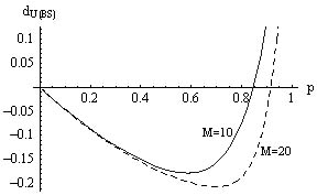
Figure 1: Variation of quantum phase fluctuation of binomial state.

From the Fig. 1, it is clear that the binomial state shows reduction of fluctuation of quantum phase with respect to its coherent state counter part and thus it satisfies this stronger criterion of nonclassicality. But it does not satisfy the criterion for higher values of $p$. In [10] we have shown that Binomial state is always antibunched up to any order. For higher values of $p$ it is antibunched in every order and thus satisfies the other strong criterion of nonclassicality but do not satisfy the criterion laid down on the basis of quantum phase fluctuations. Earlier we had reported [9] that reduction of quantum phase fluctuation means antibunching but the converse is not true. This is the first time when an example of such a state which is antibunched but reduction of quantum phase fluctuation with respect to coherent state does not happen, is found.

3.2 Generalized binomial state

As we have mentioned earlier there are different form of generalized binomial states [32-34], in the present section we have chosen generalized binomial state introduced by Roy and Roy [33] for our study. Roy and Roy have introduced the generalized binomial state as

$$|N,\alpha,\beta\rangle=\sum_{n=0}^{N}\sqrt{\omega(n,N,\alpha,\beta)}|n\rangle$$ (25)

where,

$$\omega(n,N,\alpha,\beta)=\frac{N!}{(\alpha+\beta+2)_{N}}\frac{(\alpha+1)_{n}(\beta+1)_{N-n}}{n!(N-n)!}$$ (26)

where $(x)_{r}$ is conventional Pochhammer symbol and $\alpha,\beta>-1$, $n=0,1,....,N$. Now with the help of properties of Pochhammer symbol and operator algebra we can obtain following relations:

$$\begin{array}[]{lcl}a|N,\alpha,\beta\rangle&=&\left\{\frac{N(\alpha+1)}{(\alpha+\beta+2)}\right\}^{\frac{1}{2}}\sum_{l=0}^{N-1}\left\{\frac{(N-1)!(\alpha+2)_{l}(\beta+1)_{N-1-l}}{(\alpha+2+\beta+1)_{N-1}l!(N-1-l)!}\right\}^{\frac{1}{2}}|l\rangle\\ &=&\left\{\frac{N(\alpha+1)}{(\alpha+\beta+2)}\right\}^{\frac{1}{2}}\sum_{n=0}^{N-1}\sqrt{\omega(n,N-1,\alpha+1,\beta)}|n\rangle,\end{array}$$ (27)

$$\langle N,\alpha,\beta|a^{\dagger}a|N,\alpha,\beta\rangle=\frac{N(\alpha+1)}{(\alpha+\beta+2)},$$ (28)

$$\langle N,\alpha,\beta|a^{\dagger 2}a^{2}|N,\alpha,\beta\rangle=\frac{N(N-1)(\alpha+1)(\alpha+2)}{(\alpha+\beta+2)(\alpha+\beta+3)}$$ (29)

and

$$\begin{array}[]{ccc}\left\langle a^{\dagger}\right\rangle\left\langle a\right\rangle&=&\frac{N^{2}(\alpha+1)^{2}}{(\alpha+\beta+2)^{2}}[\sum_{n=0}^{N-1}\sqrt{\omega(n,N-1,\alpha+1,\beta)}\end{array}]^{2}.$$ (30)

Therefore,

$$\begin{array}[]{lcl}d_{U(GBS)}&=&\left[\frac{(\beta+1)(\alpha+\beta+N+2)}{N^{3}(\alpha+1)(\alpha+\beta+3)[\frac{(N-1)!(\alpha+2)_{n}(\beta+1)_{N-n}}{(\alpha+\beta+3)_{N-1}(N-n-1)!}]}\right.\left[\frac{N(N-1)(\alpha+1)(\alpha+2)}{(\alpha+\beta+2)(\alpha+\beta+3)}\right.\\ &-&\left.\begin{array}[]{c}\left.\frac{N^{4}(\alpha+1)^{2}(N-1)!(\alpha+2)_{n}(\beta+1)_{N-n}}{(\alpha+\beta+2)^{2}(\alpha+\beta+3)_{N-1}(N-n-1)!}+\frac{1}{2}\right]\end{array}-\frac{1}{2}\right]\end{array}$$ (31)

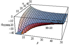
Figure 2: Variation of quantum phase fluctuation with respect to $\alpha$ and $\beta$ for Roy and Roy generalized binomial state.

From Fig. 2 it is clear that the reduction of quantum phase fluctuation happens for Roy and Roy generalized binomial state. It is also observed that the depth of nonclassicality reduces with the increase in $\alpha$ and $\beta$. But as far as the higher (second) order antibunching is concerned, the depth of nonclassicality associated with it decreases with increase in $\alpha$ and increases with increase in $\beta$ (see Fig. 2 and 3 of [10]). Farther it had been observed in [10] that for particular values of $\alpha,\beta$ and $N$ the state does not show second order antibunching. But here it is found that for the same values of $\alpha,\beta$ and $N$ we can obtain reduction of quantum phase fluctuation parameter with respect to its coherent state counterpart. Consequently we can say that, reduction of quantum phase fluctuation means antibunching but does not essentially mean higher order antibunching and therefore, it is not essential that these two stronger conditions of nonclassicality would appear simultaneously.

3.3 Photon added coherent state:

Photon added coherent state (PACS) is defined as [39])

$$\begin{array}[]{lcl}|\alpha,m>&=&\frac{exp(-|\alpha|^{2}/2)}{[L_{m}(-|\alpha|^{2})m!]^{1/2}}\sum_{n=0}^{\infty}\frac{\alpha^{n}\sqrt{(n+m)!}}{n!}|n+m>\end{array}$$ (32)

where $L_{m}(x)$$\begin{array}[]{cc}=&\sum_{n=0}^{m}\frac{(-x)^{n}m!}{(n!)^{2}(m-n)!}\end{array}$is Lauguere polynomial. Rigorous operator algebra yields

$$<a^{\dagger}a>=\frac{exp(-|\alpha|^{2})}{L_{m}(-|\alpha|^{2})m!}\sum_{n=0}^{\infty}\frac{(n+m)!\alpha^{2(n+1)}(m+n+1)^{2}}{(n+1)!^{2}},$$ (33)

$$<a^{\dagger 2}a^{2}>=\frac{exp(-|\alpha|^{2})}{L_{m}(-|\alpha|^{2})m!}\sum_{n=0}^{\infty}\frac{(n+m)!\alpha^{n+2}(m+n+1)^{2}(m+n+2)^{2}}{(n+2)!^{2}}$$ (34)

and

$$<a^{\dagger}>=<a>=\frac{exp(-|\alpha|^{2})}{L_{m}(-|\alpha|^{2})m!}\sum_{n=0}^{\infty}\frac{(n+m)!\alpha^{2n+1}(m+n+1)}{(n+1)(n!)^{2}}.$$ (35)

By substituting equations (33-35) in (16) we can easily obtain a long expression of $d_{U}$. Essential characteristic of $d_{U}$ of PACS can be seen in Fig 3. It is easy to observe that the reduction of quantum phase fluctuation is possible in photon added coherent state. Since the depth of nonclassicality increases with the increase in $m$. So we can conclude, the more photon are added to coherent state the more nonclassical it is as far as the depth of nonclassicality associated with quantum phase fluctuation is concerned. This particular characteristic is also been reflected in higher order antibunching [10].

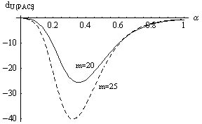
Figure 3: Variation of quantum phase fluctuation of photon added coherent state.

3.4 Other intermediate states

As it is mentioned in the earlier sections, there exist several different intermediate states. For the systematic study of possibility of reduction of quantum phase fluctuation in intermediate states, we have studied all the well known intermediate states. Since the procedure followed for the study of different states is similar, mathematical detail has not been shown in the subsections below. But from the expression of $d_{U}$ and the corresponding plots it would be easy to see that the reduction of quantum phase fluctuation can be observed in all the intermediate states studied below.

3.4.1 Negative binomial state

Negative Binomial State(NBS) can be defined as

$$|p,M\mbox{>}=\sum_{n=M}^{\infty}[\left(\begin{array}[]{c}n\\ M\end{array}\right)p^{M+1}(1-p)^{n-M}]^{1/2}|n>.$$ (36)

Similar operator algebra yields

$$d_{U(NBS)}=\left[\frac{(M+1)(1-p)^{2M+1}}{p^{2(M+2)}}\left\{\frac{\frac{(M+1-p)}{p}-\frac{p^{2(M+1)}}{(1-p)^{2M}}\left(\sum_{n=M}^{\infty}\sqrt{\left(\begin{array}[]{c}n+1\\ M\end{array}\right)\left(\begin{array}[]{c}n\\ M\end{array}\right)(1-p)^{(n+1)}(n+1)}\right)^{2}+\frac{1}{2}}{\left(\sum_{n=M}^{\infty}\sqrt{\left(\begin{array}[]{c}n+1\\ M\end{array}\right)\left(\begin{array}[]{c}n\\ M\end{array}\right)(1-p)^{(n+1)}(n+1)}\right)^{2}}\right\}-\frac{1}{2}\right].$$ (37)

Variation of quantum phase fluctuation parameter with respect to the probability $p$ for NBS is shown in the Fig. 4 and it has been observed that the state is more nonclassical for lower values of $p$ and higher values of $M$ [10]. This is consistent with the earlier observations on higher order antibunching of NBS.

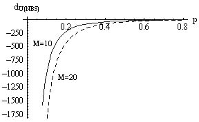
Figure 4: Variation of quantum phase fluctuation of negative binomial state.

3.5 Hyper geometric state

Hyper geometric state (HS) is defined as [36]

$$|L,M,p>=\sum_{n=0}^{M}H_{n}^{M}(p,L)|n>$$ (38)

where, $H_{n}^{M}=\left[\left(\begin{array}[]{c}Lp\\ n\end{array}\right)\left(\begin{array}[]{c}L(1-p)\\ M-n\end{array}\right)\right]^{1/2}\left(\begin{array}[]{c}L\\ M\end{array}\right)^{-1/2}$. For this intermediate state we obtain

$$\begin{array}[]{lcl}d_{U(HS)}&=&\left[\frac{pM(1-p)(L-M)\left(\begin{array}[]{c}L\\ M\end{array}\right)^{2}}{(L-1)\sqrt{Lp}\left(\sum_{n=0}^{M-1}\sqrt{\left(\begin{array}[]{c}Lp\\ n\end{array}\right)\left(\begin{array}[]{c}L(1-p)\\ M-n\end{array}\right)\left(\begin{array}[]{c}Lp-1\\ n\end{array}\right)\left(\begin{array}[]{c}L(1-p)\\ M-n-1\end{array}\right)}\right)^{2}}\right.\\ &\times&\left.\left\{Mp-\frac{\sqrt{Lp}}{\left(\begin{array}[]{c}L\\ M\end{array}\right)^{2}}\left(\sum_{n=0}^{M-1}\sqrt{\left(\begin{array}[]{c}Lp\\ n\end{array}\right)\left(\begin{array}[]{c}L(1-p)\\ M-n\end{array}\right)\left(\begin{array}[]{c}Lp-1\\ n\end{array}\right)\left(\begin{array}[]{c}L(1-p)\\ M-n-1\end{array}\right)}\right)^{2}+\frac{1}{2}\right\}-\frac{1}{2}\right].\end{array}$$ (39)

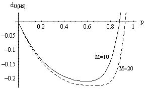
Figure 5: Variation of quantum phase fluctuation of hyper geometric state.

Fig. 5 depicts the characteristics of quantum phase fluctuation of HS. From this figure we can clearly observe that HS does not satisfy the reduction of quantum phase fluctuation criterion for higher values of $p$ but it satisfies the condition of higher order antibunching and consequently the condition of antibunching for those values of $p.$ This is consistent with our theoretical prediction that reduction of quantum phase fluctuation means antibunching but the converse is not true.

4 Conclusions

In essence, all the intermediate states described above show reduction of $U$ with respect to its coherent state value. This establishes that the intermediate states can satisfy the stronger criterion of nonclassicality compared to the criterion of usual antibunched state. This is consistent with our earlier observation of higher order antibunching of intermediate states [10]. Further, we would like to note that the binomial state can show reduction of fluctuation of quantum phase with respect to its coherent state counter part and thus it can satisfy this stronger criterion of nonclassicality. But it does not satisfy the criterion for higher values of $p$ (see Fig. 1). In [10] we have shown that Binomial state is always antibunched up to any order. Thus for higher values of $p$ it is higher order antibunched and consequently satisfies the other strong criterion of nonclassicality but do not satisfy the criterion laid down on the basis of quantum phase fluctuations. Similar phenomenon is also observed in HS. Earlier we had reported [9] that reduction of quantum phase fluctuation means antibunching but the converse is not true. This is the first time when an example of such a state which is antibunched but does not show reduction of quantum phase fluctuation with respect to coherent state, is found. Further from the study of phase properties of Roy Roy GBS and HS we have learnt that the reduction of quantum phase fluctuation mean antibunching but does not essentially mean higher order antibunching and therefore, it is not essential that these two stronger conditions of nonclassicality appear simultaneously. In connection to PACS we have observed that the more photon are added to coherent state the more nonclassical the PACS, is as far as the depth of nonclassicality associated with quantum phase fluctuation is concerned. This particular characteristic has also been reflected in higher order antibunching [10]. Further we have seen that the NBS is more nonclassical for lower values of $p$. This is also similar with the earlier observations on higher order antibunching of NBS.

Acknowledgement: AP thanks to DST, India for partial financial support through the project grant SR\FTP\PS-13\2004.

References

1. Orlowski A, Phys. Rev. A 48 (1993) 727.

2. Hanbury-Brown R, Twiss R Q, Nature 177 (1956) 27.

3. Dodonov V V, J. Opt. B. Quant. and Semiclass. Opt. 4 (2002) R1.

4. P. Carutherrs and M. M. Nieto, Rev. Mod. Phys. 40 (1968) 411.

5. C. C. Gerry, Opt. Commun., 63 (1987) 278.

6. C. C. Gerry, Opt. Commun., 75 (1990) 168.

7. R. Lynch, Opt. Commun., 67 (1988) 67.

8. A. Pathak and S. Mandal, Phys. Lett. A 272 (2000) 346.

9. P Gupta and A Pathak, Phys. Lett. A 365 (2007) 393.

10. A Verma, N K Sharma and A Pathak, quant-ph\0706.0697.

11. A. Pathak and M. E. Garcia, Appl. Phys. B 84 (2006) 479.

12. R. Lynch, Phys. Reports 256 (1995) 367.

13. L. Suskind and J. Glogower, Physics 1 (1964) 49.

14. D. T. Pegg and S. M. Barnett, Phys. Rev. A 39 (1989) 1665.

15. S. M. Barnett and D. T. Pegg, J. Phys. A 19 (1986) 3849.

16. Fan Hong-Yi and H. R. Zaidi, Opt. Commun., 68 (1988) 143.

17. B. C. Sanders, S. M. Barnett and P. L. Knight, Opt. Commun., 58 (1986) 290.

18. D. Yao, Phys. Lett. A, 122 (1987) 77.

19. R. Lynch, J. Opt. Soc.Am, B4 (1987) 1723.

20. J. A. Vaccaro and D. T. Pegg, Opt.Commun., 70 (1989) 529.

21. Y. K. Tsui, Phys Rev. A 47 12296 (1993).

22. Hong C K and Mandel L, Phys. Rev. Lett. 54 (1985) 323.

23. Lee C T, Phys. Rev. A 41 (1990) 1721.

24. M. Hillery, Phys. Rev. A 36 (1987) 3796.

25. A B Klimov et al, J. Phys. A 37 (2004) 4097.

26. L. L. Sanchez-Soto et al Phys. Rev. A 66 (2002) 042112.

27. I. Iguchi, T. Yamaguchi and A. Sugimato Nature 412 (2001) 420 .

28. A Zavatta, S Viciani, M Bellini, Science 306 (2004) 660.

29. P. A . M. Dirac, Proc. Royal. Soc. London Ser. A 114 (1927) 243.

30. W. H. Louisell, Phys. Lett. 7 (1963) 60.

31. D Stoler, B E A Saleh and M C Teich, Opt. Acta 32 (1985) 345.

32. Hong-Chen Fu and Ryu Sasaki J. Phys. A 29 (1996) 5637.

33. P Roy and B Roy, J. Phys. A 30 (1997) L719.

34. Hong-Yi Fan and Nai-le Liu, Phys. Lett. A 264 (1999) 154.

35. A S F Obada, M Darwish and H H Salah, Int. J. Theo. Phys. 41 (2002) 1755.

36. H. C. Fu and R. Sasaki, J. Math. Phys. 38 (1997) 2154.

37. H Fan and N Liu, Phys. Lett. A 250 (1998) 88.

38. M H Y Moussa and B Baseia, Phys. Lett. A 238 (1998) 223.

39. G S Agarwal and K Tara, Phys. Rev. A 43 (1991) 492.

40. C Valverde et al, Phys. Lett. A 315 (2003) 213.

41. R Lo Franco et al, Phys. Rev. A 74 (2006) 045803.