Realistic Equations of State for the Primeval Universe

Abstract

Early universe equations of state including realistic interactions between constituents are built up. Under certain hypothesis, these equations are able to generate an inflationary regime prior to the nucleosynthesis period. The resulting accelerated expansion is intense enough to solve the flatness and horizon problems. In the cases of curvature parameter $\kappa$ equal to $0$ or $+1$, the model is able to avoid the initial singularity and offers a natural explanation for why the universe is in expansion. All the results are valid only for a matter-antimatter symmetric universe.

2008 number number identifier Date text]date LABEL:FirstPage1 LABEL:LastPage#1

I Introduction

The gravitational field, as described by General Relativity, couples to all types of energy: rest masses, kinetic terms and interaction terms. Relativistic cosmology is, in consequence, deeply concerned with such sources. The kinetic terms and the rest-masses are currently taken into account by assuming ideal cosmic fluids constituted by ultrarelativistic and/or non-relativistic matter. Solutions of this type are found in standard texts nar ; wein and – when multi-component fluids are considered – in several papers, e.g., Solutions . Interaction terms are commonly used only in perturbative models. In fact, using the Boltzmann equation in a Friedmann-Robertson-Walker (FRW) background, the inhomogeneities both in the cosmic microwave background (CMB) and in the matter content Dod ; kolb are studied, for comparison with the observational data Wmap ; LargeScale . Notwithstanding, interactions are not considered as direct sources of gravitation in this line of research artigo 1 .

Of course, some well-known proposals do consider interaction processes as direct sources of gravitation. They are usually related to the accelerated expansion regimes: present-day dynamics SuNo or inflation Liddle . Nevertheless, these theories do not actually consider the fundamental interactions (electromagnetic, weak and strong) between particles in the source constituents. Indeed, in the standard inflationary approaches Guth ; AlbreSten ; Linde an accelerated expansion is obtained through self-interaction processes of scalar inflaton fields $\phi_{i}\left(x\right)$. This self-interaction is chosen so as to produce just those features which are necessary to describe the early accelerated regime Liddle . The phenomenological explanations for the present-day acceleration include, among others, (i) the quintessence models CalDaveStein ; Stein ; Zlatev ; FraRos ; PeRa , which roughly follow the same lines of the inflationary theory; (ii) models of matter and dark-energy unification via Chapligyn-like equations of state (EOS) Orfeu or through equations of the Van der Walls type Capozzielo ; Kremer ; (iii) models of mass-varying-neutrino type, which couple neutrinos to a quintessence scalar field Motta ; (iv) models introducing interactions in the energy conservation equation Gabi ; NelsonPinto .

A formal procedure has been recently proposed for including the (fundamental) interactions as direct sources of gravitation in the cosmological context artigo 1 . Imported from equilibrium statistical mechanics, this formalism allows the construction of realistic equations of state for both relativistic Dashen ; Reichl and non-relativistic systems Pat ; Beth . Our objective here is to find primeval cosmic fluid EOS taking into account physically realistic interaction processes between the constituent particles, in addition to their kinetic and rest-mass terms. In particular, we shall examine their effect on the scale factor evolution. It will be shown that under certain hypothesis and approximations an early accelerated regime can be obtained as a consequence of these interacting processes.

The idea of building realistic equations of state considering interaction between elementary particles in the primeval universe is not new. Actually, during the late 1970’s and the beginning os the 80’s a series of papers by Bugrii, Trushevsky and Beletsky ucraone ; ucratwo ; ucrathree ; ucrafour discussed the construction of the high-energy EOS and their application to the pre-nucleosynthesis universe. Nevertheless, their treatment is different from the one developed here as we will make clear some pages ahead.

The paper is organized as follows. Section II reviews the general features of the early universe in its standard presentation nar ; wein ; Dod ; kolb ; Liddle . Section III presents some results from equilibrium statistical theory of interacting systems. Specifically, the coefficients appearing in the perturbative fugacity expansions are expressed in terms of the scattering matrix operator $\hat{S}$. In addition, the matrix $S_{2}$ describing the two-particle scattering is associated to the experimentally observable phase-shifts. The goal of Section IV is to construct realistic EOS for the pre-nucleosynthesis universe and discuss the hypothesis and approximations undertaken. In Section V, the more direct cosmological consequences coming from these equations are examined, including the effect of driving an accelerated expansion (inflationary era). Section VI contains some final comments. Details of a too technical nature, as well as some data, have been relegated to appendices.

II General features of the pre-nucleosynthesis universe

The period of the Universe evolution going under the name “Early Universe” covers many different and physically significant events. Indeed, it is usual to consider both the matter-radiation decoupling ($kT_{\gamma}\sim 0.1$ $eV$) and the electroweak transition ($kT_{\gamma}\sim 100$ $GeV$) as belonging to that period. This work is concerned with a specific interval within it, namely the pre-nucleosynthesis period (PNS). We shall define PNS as the period immediately before the nucleosynthesis of the light elements, when the nucleons (protons and neutrons) are in thermodynamical equilibrium with the rest of the cosmic fluid, i.e., $kT_{\gamma}\gtrsim 20$ $MeV$. So, in principle, any energy value larger than $20$ $MeV$ belongs to PNS; nevertheless, it will be enough to restrict our working frame to energies of a few hundreds of $MeV$. In consequence, PNS will in what follows actually mean the interval $20$ $MeV\leq kT\lesssim 300$ $MeV$.

Present-day universe is dominated by a dark energy component $\Lambda$ plus a non-relativistic contribution formed by ordinary baryons $b$ and dark-matter $dm$; the ultrarelativistic components – photons $\gamma$ and neutrinos $\nu$ – are quite negligible. As one goes back in time, however, this situation changes drastically. Indeed, the evolution equations for ultrarelativistic and the nonrelativistic matter nar ; wein in terms of the expansion parameter,

$$\rho_{\gamma,\nu}=\rho_{\gamma 0,\nu 0}\left(\frac{a_{0}}{a}\right)^{4}\text{ \ \ \ \ and \ \ \ }\rho_{b,DM}=\rho_{b0,DM0}\left(\frac{a_{0}}{a}\right)^{3},$$ (1)

together with the Friedmann equations,

$$\left(\frac{\dot{a}}{a}\right)^{2}=\frac{8\pi G}{3}\rho-\frac{\kappa}{a^{2}}+\frac{\Lambda}{3}\text{ \ \ \ and \ \ \ }\left(\frac{\ddot{a}}{a}\right)=-\frac{4\pi G}{3}\left(\rho+3p\right)+\frac{\Lambda}{3},$$ (2)

show that the ultrarelativistic contribution overcomes that of the other components at energies corresponding to $kT_{\gamma}\sim 1$ $eV$. The cosmological period dominated by ideal ultrarelativistic particles is usually called the radiation era.

To find out the energetically relevant constituents during the PNS period we must notice that, as we turn to the past and the energy $kT$ increases, pair-production processes become more and more frequent, generating a large variety of particles. The main scenario is that of ultrarelativistic particles generating non-relativistic ones. If we restrict ourselves to a few hundreds of $MeV$, the relevant particles are:

• fundamental bosons: photons $\left(\gamma\right)$;

• leptons: electrons $\left(e^{-}\right)$, positrons $\left(e^{+}\right)$, muons $\left(\mu^{-}\right)$, antimuons $\left(\mu^{+}\right)$, electronic and muonic neutrinos $\left(\nu_{e},\nu_{\mu}\right)$ and electronic and muonic antineutrinos $\left(\bar{\nu}_{e},\bar{\nu}_{\mu}\right)$;

• hadrons: pions $\left(\pi^{+},\pi^{-},\pi^{0}\right)$, kaons $(K^{+},K^{-},K^{0},\bar{K}^{0})$, nucleons $\left(p,n\right)$ and antinucleons $\left(\bar{p},\bar{n}\right)$.

Concerning this list, it is important to emphasize that: (i) the particles taken into account are those with rest-mass bellow $1$ $GeV$; and, (ii) the hadrons considered are only those which are stable by the strong interaction. Furthermore, we assume matter-anti-matter symmetry.

Among the particles cited above, those that are ultrarelativistic at $20$ $MeV$ are $\gamma$, $e^{\pm}$, $\nu_{e}$, $\nu_{\mu}$, $\bar{\nu}_{e}$ and $\bar{\nu}_{\mu}$; the remaining ones are non-relativistic. By arguments given in classical texts nar ; wein ; kolb , the chemical potentials involved in the PNS reactions are zero, i.e., $\mu_{i}\simeq 0$ for every species ($i=\gamma$, $e^{\pm}$, $\mu^{\pm}$, $\pi^{\pm}$, $K^{\pm}$, …).

Thermal equilibrium is warranted as long as every reaction rate $\Gamma_{i}(kT)$ of each given component $i$ with all the other particles is much larger than the universe expansion rate. This last, in turn, is measured by the Hubble function $H(kT)$. Therefore, when the condition

$$\Gamma(T)\gg H(T)$$ (3)

is satisfied, thermodynamical quasi-static expansion holds. In fact, this may be verified for each variety by remembering that $\Gamma=n\sigma\left|\vec{v}\right|$, where $n$ is the target-particle density and $\sigma\left|\vec{v}\right|$ is the interaction cross-section times the relative velocity of the particles. The presence of thermal and chemical equilibria in PNS is extremely convenient, as it enables us to adopt, in the comoving reference frame, the usual statistical mechanics on the $\mathbf{E}^{3}$ manifold (the phase space measure is given simply by $\frac{1}{\left(2\pi\right)^{3}}\iint d^{3}xd^{3}p$).

The energy density turning up in (2) is nar ; kolb

$$\rho_{UR}=\rho_{\gamma}+\rho_{e^{-}}+\rho_{e^{+}}+\rho_{\nu_{e}}+\rho_{\nu_{\mu}}+\rho_{\bar{\nu}_{e}}+\rho_{\bar{\nu}_{\mu}}=\frac{9}{2}\,\rho_{\gamma}=\frac{9\pi^{2}}{30}(kT)^{4}$$ (4)

and can be used to obtain the Hubble function as a function of $kT$:

$$H(kT)=\left(\frac{\dot{a}}{a}\right)=\sqrt{\frac{4\pi^{3}}{5}}\,\frac{(kT)^{2}}{m_{Pl}},$$ (5)

where $m_{Pl}\equiv G^{-1/2}=1.221\times 10^{22}$ $MeV$. The relation between the scale factor and the energy $kT$ is determined by comparing (4) to (1):

$$kT=\frac{A}{a}\,\,.$$ (6)

$A$ is a constant which depends on the present–day values $T_{0}$ and $a_{0}$. Substituting this last equation into (5) and solving the resulting differential equation – imposing the initial condition $a(t=0)=0$ – leads to

$$a(t)=A\left(\frac{16\pi^{3}}{5}\right)^{1/4}\left(\frac{t}{m_{Pl}}\right)^{1/2}.$$ (7)

From (6) follows then the relation between the energy $kT$ and the cosmological time $t$:

$$kT=\left(\frac{16\pi^{3}}{5}\right)^{-1/4}\left(\frac{t}{m_{Pl}}\right)^{-1/2}$$ (8)

The last four equations determine the evolution of the primeval universe in a radiation–dominated era.

III Statistics of interacting systems

It was discussed elsewhere artigo 1 how to construct equations of state for an interacting system of particles within the standard ensemble formalism of statistical mechanics, and how this could be applied to a simple model relevant to cosmology. In what follows, we will present a brief review of the information needed here. We also indicate Refs. Dashen , Beth , mayer and LeeYang for further information.

The grand canonical partition function $\Theta$ is expressed as

$$\Theta(z,V,T)=\sum\limits_{N=0}^{\infty}Q_{N}(V,T)z^{N},$$ (9)

where $V$ is the volume, $T$ is the temperature, $z=e^{\mu/kT}$ is the fugacity and $Q_{N}(V,T)$ is the N-particle canonical partition function. The chemical potential $\mu=\mu^{NR}+m$ is composed by the rest mass $m$ plus the non-relativistic chemical potential $\mu^{NR}$. This last is that usually found in standard statistical mechanics texts, e.g. Pat . Here, we are concerned only with one-component systems. For the cases of more constituents, see Appendix A.

The thermodynamical quantities – pressure $p$, energy density $\rho$, numerical density $n$, etc. – are related to the grand canonical potential

$$\Omega(z,T)\equiv\frac{1}{V}\ln\Theta(z,V,T)=\sum\limits_{N=1}^{\infty}b_{N}z^{N},$$ (10)

written in terms of the cluster integrals $b_{N}$. The thermodynamical limit has already been taken in Eq. (10), so that the $b_{N}$ are functions of the temperature solely (the $V$ dependence disappears). According to Dashen, Ma and Bernstein Dashen , the cluster integrals are calculated from the $S$-matrix as follows:

$$b_{N}-b_{N}^{(0)}=\frac{g_{N}}{V}\int\frac{e^{-\beta E}}{4\pi i}Tr\left(\hat{A}\hat{S}^{-1}\frac{\overleftrightarrow{\partial}}{\partial E}\hat{S}\right)_{\tilde{c}_{N}}dE,$$ (11)

where $\beta=1/kT$, $g_{N}$ counts the degeneracy coming from internal degrees of freedom, $\hat{A}$ symmetrizes (antisymmetrizes) the bosonic (fermionic) states, $\hat{S}$ is the scattering matrix operator and $b_{N}^{(0)}$ is the cluster integral of the non-interacting quantum system. The subscript $\tilde{c}_{N}$ represents all the $N$-particle connected diagrams in which the interaction occurs at least once. In (11), it was used the short-cut

$$\hat{S}^{-1}\frac{\overleftrightarrow{\partial}}{\partial E}\hat{S}\equiv\hat{S}^{-1}\frac{\partial\hat{S}}{\partial E}-\frac{\partial\hat{S}^{-1}}{\partial E}\hat{S}.$$ (12)

By using (10) $p$, $n$ and $\rho$ are determined as series in the fugacity:

$$\frac{p(z,T)}{kT}=\sum\limits_{N=1}^{\infty}b_{N}z^{N}~{};\text{ \ }n(z,T)=\sum\limits_{N=1}^{\infty}Nb_{N}z^{N};\text{ \ }\rho(z,T)=-\sum\limits_{N=1}^{\infty}\frac{\partial b_{N}}{\partial\beta}z^{N}.$$ (13)

This is the parametric form of the equations of state.

An alternative description is given by the pressure $p(n,T)$ and the energy density $\rho(n,T)$ written in terms of $n\left(z,T\right)$. They are obtained by inversion of series $n\left(z,T\right)$ and substitution into $p(z,T)$ and $\rho(z,T)$. This results in the virial expansion:

$$\frac{p(n,T)}{kT}=\sum_{l=1}^{\infty}a_{l}(T)n^{l};\ \ \ \frac{\rho(n,T)}{\left(kT\right)^{2}}=\sum_{l=1}^{\infty}c_{l}(T)n^{l},$$ (14)

with $a_{l}$ and $c_{l}$ representing the virial coefficients for the pressure and the energy density. These coefficients are completely determined by the $b_{N}$. Appendix A presents the explicit forms of $a_{l}$ and $c_{l}$ for a two-component system.

In practice, it is not possible to really sum any of the series (13-14). Therefore, the choice of using $p$ and $\rho$ in terms of $z$ or $n$ depends on the perturbative characteristics of each series and on the system under study. We will return to this question in Section IV.

III.1 The second coefficient of the fugacity expansion

The elastic interaction between two particles is decomposed into rotation–invariant sectors, so that each part depends only on their relative distance $r$ (central interaction):

$$\hat{V}^{a}(r)\equiv\hat{H}^{a}-\hat{H}^{(0)a},$$ (15)

index $a$ standing for the other types of invariance: spin, isospin, charge conjugation, etc. The scattering matrix $S_{2}^{a}$ depends then only on the energy and the angle between the initial and final momenta. In this angular momentum representation, the $\hat{S}_{2}^{a}$ operator can be written solely in terms of the phase shifts $\delta_{l}^{a}(k)$:

$$\left\langle k^{\prime}l^{\prime}m^{\prime}\right|\hat{S}_{2}^{a}\left|klm\right\rangle=e^{2i\delta_{l}^{a}(k)}\delta_{k^{\prime},k}\delta_{l^{\prime},l}\delta_{m^{\prime},m}.$$ (16)

The symmetrization performed by operator $\hat{A}$ in (11) must account for the complete state associated with $a$. It is possible to transfer this symmetrization instruction to the index $a$. Once this is done, the cluster integral of the two-particle system is written as

$$b_{2}-b_{2}^{(0)}=\sum\limits_{a}\frac{g_{2}^{a}}{V}\int\frac{dE}{4\pi i}e^{-\beta E}Tr\left[\left(\hat{S}_{2}^{a}\right)^{-1}\frac{\overleftrightarrow{\partial}}{\partial E}\hat{S}_{2}^{a}\right],$$ (17)

where $g_{2}^{a}$ counts the degeneracy degree of the duly symmetrized states.

If we carry out a coordinate transformation to the center of mass, the state will behave just like a free state (plane wave), that is, it will obey the free Hamiltonian. In order to explore this fact, we remember some properties of the relativistic invariant $s$:

$$\omega^{2} \equiv s=\left(p_{1\mu}+p_{2\mu}\right)^{2}=m_{1}^{2}+m_{2}^{2}+2p_{1\mu}p_{2}^{\mu}$$

$$=E_{1}^{2}+E_{2}^{2}+2E_{1}E_{2}-\left(\vec{p}_{1}+\vec{p}_{2}\right)^{2}=E^{2}-\vec{P}^{2},$$ (18)

$m_{1}$ and $m_{2}$ are the masses of the two particles, $E=E_{1}+E_{2}$ is the sum of their energy, and the momentum of the center of mass is $\vec{P}\equiv\vec{p}_{1}+\vec{p}_{2}$. Since $E$ and $\vec{P}$ are the energy and the momentum of the two-particle cluster, $\omega$ may be understood as the mass of this cluster and encapsulates all the information about the interaction. As the interaction calculated by (17) does not depend on the coordinates of the center of mass, the integration and the differential operator with respect to $E$ are reexpressed as

$$b_{2}-b_{2}^{(0)}=\sum\limits_{a}\frac{g_{2}^{a}}{V}\int d^{3}R\int\frac{d^{3}P}{\left(2\pi\right)^{3}}\int\frac{d\omega}{4\pi i}e^{-\beta\sqrt{\vec{P}^{2}+\omega^{2}}}Tr\left[\left(\hat{S}_{2}^{a}\right)^{-1}\frac{\overleftrightarrow{\partial}}{\partial\omega}\hat{S}_{2}^{a}\right].$$ (19)

The next step is to integrate on $d^{3}P$:

$$b_{2}-b_{2}^{(0)}=\sum\limits_{a}\frac{g_{2}^{a}}{2\beta\pi^{2}}\int\limits_{M}^{\infty}\omega^{2}K_{2}(\beta\omega)\frac{1}{4\pi i}Tr\left[\left(\hat{S}_{2}^{a}\right)^{-1}\frac{\overleftrightarrow{\partial}}{\partial\omega}\hat{S}_{2}^{a}\right]d\omega,$$ (20)

where $M=m_{1}+m_{2}$ is the minimum value assumed by $\omega$; $K_{2}(\beta\omega)$ is the modified Bessel function. Using (16), the trace in the angular momentum representation is

$$Tr\left[\left(\hat{S}_{2}^{a}\right)^{-1}\frac{\overleftrightarrow{\partial}}{\partial\omega}\hat{S}_{2}^{a}\right]=4i\sum\limits_{l=0}^{\infty}\left(2l+1\right)\frac{\partial\delta_{l}^{a}(\omega)}{\partial\omega}\,\,.$$ (21)

Equation (20) becomes:

$$b_{2}-b_{2}^{(0)}=\frac{1}{2\beta\pi^{3}}\sum\limits_{a}\sum\limits_{l=0}^{\infty}g_{2}^{a}\left(2l+1\right)\int\limits_{M}^{\infty}\omega^{2}K_{2}(\beta\omega)\frac{\partial\delta_{l}^{a}(\omega)}{\partial\omega}d\omega.$$ (22)

This equation, which reduces to the Beth – Uhlenbeck Beth ; Pat case in the non-relativistic limit, is the fundamental tool to obtain the EOS for the pre-nucleosynthesis universe.

IV Equations of state for the pre-nucleosynthesis universe

The EOS to be built here are supposedly realistic because they account for the interactions. Nevertheless, we will not actually consider all the four fundamental interactions.

The gravitational interaction is accounted for only through Einstein (more specifically, Friedmann) equations. We will neglect any possible change in the description of statistical mechanics due to the curved background of the cosmic manifold.

The electromagnetic interaction, though responsible for the thermalization of the charged particles, will not be relevant to the primeval EOS, since: (i) the shielding effect due to the existence of opposite charges makes it possible to consider the effective interaction as of short range, and the fluid as neutral; (ii) the coupling constant of the electromagnetic interaction is relatively small ($e^{2}\sim 1/137$). The mean interaction energy between charged particles is nearly two orders of magnitude lesser than their mean kinetic energies nar . The weak interaction, though responsible for the thermalization of the neutral particles, is of short-range, and its intensity is much smaller Grif than the strong interaction. It will be neglected. Due to its high coupling constant, and despite its short-range, the strong (“hadronic”) interaction is dominant in the PNS period. As a matter of fact, it is the only one that will be taken into account (see Appendix B).

Justified by these considerations, we divide the relevant particles for the PNS in three categories:

1. Ideal ultrarelativistic particles: $\gamma,e^{-},e^{+},\nu_{e},\nu_{\mu},\bar{\nu}_{e},\bar{\nu}_{\mu}$;

2. Ideal relativistic particles: $\mu^{-},\mu^{+}$;

3. Interacting relativistic particles: $\pi^{+},\pi^{-},\pi^{0},K^{+},K^{-},K^{0},\bar{K}^{0},p,\bar{p},n,\bar{n}$.

The equations of state for such a system of particles is the sum of the contributions of each species to quantities $p$ and $\rho$, keeping in mind what has been said in Section III whenever interactions are important. Both $p$ and $\rho$ can be written as functions of $(z,T)$ or in terms of $(n,T)$ – Eqs. (13-14). Thus, there are four pairs $\left\{p,\rho\right\}$ given by the combination of $p(z,T)$, $p(n,T)$, $\rho(z,T)$ and $\rho(n,T)$. We have to decide which combination is the most suitable.

There are strong theoretical arguments (based on the series convergences) and outstanding experimental indications artigo 1 ; Hirshefeld that the virial expansion $p(n,T)$ is the most convenient form for the pressure. The choice between $\rho(z,T)$ and $\rho(n,T)$ is more subtle. We shall keep the form $\rho(z,T)$ since it maintains the probabilistic notion inherited by statistical mechanics. In fact, the energy density is a mean weighted by the Boltzmann factor, and in the case of the grand canonical ensemble it reads

$$\rho=\frac{E}{V}=\frac{1}{\Theta(V,T,z)}\sum\limits_{a,r}\frac{E_{a}}{V}e^{-\beta E_{a}}z^{N_{r}}.$$ (23)

Comparing this equation to (10) and (13) one sees that only $\rho(z,T)$ preserves the probabilistic character order by order.

Hence, the EOS for the relativistic particles (interacting or not) will be formed by the virial series for the pressure and the fugacity series for the energy density: $\left\{p(n,T),\rho(z,T)\right\}$. Only the first terms of the expansions will be considered, as only two-by-two interactions can be calculated or experimentally measured. Following the classification above, the pressure and energy density will be

$$p = p_{Had}+p_{R}+p_{UR}=p_{Had}+p_{R}+\frac{\rho_{UR}}{3},$$ (24)

$$\rho = \rho_{Had}+\rho_{R}+\rho_{UR},$$ (25)

where the labels $Had$, $R$ and $UR$ represents the hadrons, the ideal relativistic particles and the ideal ultrarelativistic particles.

IV.1 EOS for the hadrons

Pions $\pi^{+},\pi^{-},\pi^{0}$, kaons $K^{+},K^{-},K^{0},\bar{K}^{0}$ and nucleons $N=p,\bar{p},n,\bar{n}$ exhibit spin, isospin and charge conjugation symmetries under strong interactions (Appendix B). For this reason, the set of hadrons can be treated as an interacting system of three components – $\pi$, $K$ and $N$ – whose EOS are derived from (46c) and (47a). The energy density will be

$$\rho_{Had}(z_{\pi},z_{K},z_{N},kT) = \left(kT\right)^{2}\left[\dot{b}_{1\pi}z_{\pi}+\dot{b}_{1K}z_{K}+\dot{b}_{1N}z_{N}+\right.$$ (26)

$$\left.+\dot{b}_{2\pi\pi}z_{\pi}^{2}+\dot{b}_{2KK}z_{K}^{2}+\dot{b}_{2NN}z_{N}^{2}+\right.$$

$$\left.+\dot{b}_{2\pi K}z_{\pi}z_{K}+\dot{b}_{2\pi N}z_{\pi}z_{N}+\dot{b}_{2KN}z_{K}z_{N}\right],$$

where the dot indicates differentiation with respect to $kT$. To this point we have not used the fact (already discussed) that $\mu_{\pi}\simeq\mu_{K}\simeq\mu_{N}\simeq 0$ during the pre-nucleosynthesis period, and consequently $z_{\pi}\simeq z_{K}\simeq z_{N}\simeq 1$. The pressure is

$$p_{Had}(n_{\pi},n_{K},n_{N},kT) = kT\left(a_{1\pi}n_{\pi}+a_{1K}n_{K}+a_{1N}n_{N}+\right.$$ (27)

$$\left.+a_{2\pi\pi}n_{\pi}^{2}+a_{2KK}n_{K}^{2}+a_{2NN}n_{N}^{2}+\right.$$

$$\left.+a_{2\pi K}n_{\pi}n_{K}+a_{2\pi N}n_{\pi}n_{N}+a_{2KN}n_{K}n_{N}\right),$$

with the numerical densities given by

$$n_{\pi}(z_{\pi},z_{K},z_{N},kT) = b_{1\pi}z_{\pi}+2b_{2\pi\pi}z_{\pi}^{2}+b_{2\pi K}z_{\pi}z_{K}+b_{2\pi N}z_{\pi}z_{N},$$ (28)

$$n_{K}(z_{\pi},z_{K},z_{N},kT) = b_{1K}z_{K}+2b_{2KK}z_{K}^{2}+b_{2\pi K}z_{\pi}z_{K}+b_{2KN}z_{K}z_{N},$$ (29)

$$n_{N}(z_{\pi},z_{K},z_{N},kT) = b_{1N}z_{N}+2b_{2NN}z_{N}^{2}+b_{2\pi N}z_{\pi}z_{N}+b_{2KN}z_{K}z_{N}.$$ (30)

The explicit form of the ideal and interaction-related terms are given in Appendix A. The rest mass adopted are: $m_{\pi}=0.1396$ $GeV$, $m_{K}=0.4957$ $GeV$ and $m_{N}=0.93826$ $GeV$.

In principle, the term $b_{2}$ should contain all the interaction processes involving the two particles to which it refers. That is, it should describe the elastic and inelastic scatterings as well as the bound states. Actually, it is possible to argue that, in the construction of the EOS for the pre-nucleosynthesis period, bound states and inelastic processes are negligible when compared to the elastic channels.

Taking into account just the elastic processes, the six interaction terms ($\pi\pi$, $\pi K$, $\pi N$, $KK$, $KN$ and $NN$) are given by equations of type (22). The explicit expression of the cluster integrals are obtained with the help of all the phase-shift data sets – see Appendix B for an example. It is necessary to perform an integration involving the modified Bessel function $K_{2}$ and derivatives of the phase-shifts. The six integrations have been done numerically with the software Mathematica 5.0. Before that, we carefully put back the constants $c$ and $\hbar$ in such a way that the length and energy units were $fm$ and $GeV$, respectively.

The higher limits of the integrals are different for each $b_{2}$, since the phase-shift data sets are obtained in different energy intervals. Still, most of them lie in the interval from $1$ $GeV$ to $2.5$ $GeV$. As the relevant temperature values for our studies are in the range $20$ $MeV\leq kT\lesssim 300$ $MeV$, the chosen values for the higher limits are good enough to include all the main contribution from the integral kernels. Besides, the Bessel function $K_{2}$ assures the fast decrease of the kernel values. We consider only angular momenta $l=0,1$ and $2$, i.e., the $S$ , $P$ and $D$ contributions (Appendix B). Once the coefficients $b_{1}$ and $b_{2}$ have been calculated, it is straightforward to obtain the numerical densities (28), (29) and (30), and the equations of state for the hadrons, Eqs. (26) and (27).

The approach described above is not the only one for building hadronic EOS at few hundreds of $MeV$. There is also the treatment called Hadron Resonance Gas (HRG) Munzinger ; Andro ; tawfik2 ; Cheng describing the Fireballs created in the Heavy Ion Colliders (SPS – Super Proton Synchroton – and RHIC – Relativistic Heavy Ion Collider). This technique agrees qualitatively with the Lattice QCD calculations Cheng and it reproduces the abundance of the observed particles relatively well Andro . The HRG modeling is equivalent to ours as long as the ideal terms are concerned, but the procedure of including the interaction is rather different. The Hadron Resonance Gas accounts for interaction by introducing a excluded volume term a la Van der Walls Yen and by considering the resonance contributions Munzinger ; Andro . On the other hand, our work accounts for interactions through the phase shifts. Because of this, other effects – besides the ones related to resonances and hard cores (excluded volumes) – are considered. Reference Delta analyzes these features in detail for the case of $\Delta$ resonance in the $\pi N$ interaction. It is worth to emphasize that in our approach the resonances are only characteristics of the elastic scattering between stable hadrons; the resonances are not taken as particles.

In connection with what we said in the Introduction: the construction of hadronic EOS through the S-Matrix was already implemented in Refs. ucraone ; ucratwo . However, the only processes considered there (e.g. ucraone ) are those including the nucleons (scattering $NN$). The present work is more constructive and complete in this sense: all the important statistical quantities – pressure, energy density and numerical density – are obtained from the partition function which accounts for all the relevant processes of interaction two by two (scattering $\pi\pi$, $\pi K$, $\pi N$, $KK$, $KN$ and $NN$).

IV.2 EOS for the ideal particles

The ideal (non-interacting) particles are divided into two categories: ultrarelativistic ($\gamma,e^{-},\allowbreak e^{+},\nu_{e},\nu_{\mu},\bar{\nu}_{e},\bar{\nu}_{\mu}$) and relativistic ($\mu^{-},\mu^{+}$). The ultrarelativistic sector is relatively simple, and has been discussed in Section II. The calculation for the relativistic sector is analogous to what we have done for the hadrons. The energy density, for instance, is

$$\rho_{R}(z_{\mu},kT)=\left(kT\right)^{2}\left[\dot{b}_{1\mu}^{(0)}z_{\mu}+\dot{b}_{2\mu}^{(0)}z_{\mu}^{2}\right].$$ (31)

The $b_{1\mu}^{(0)}$ and $b_{2\mu}^{(0)}$ are the ideal terms determined by (51a) and (51b), with $m_{\mu}=0.10566$ $GeV$. As in the hadronic case, we set $z_{\mu}\simeq 1$ during the PNS. The pressure is

$$p_{R}(n_{\mu},kT)=kT\left[a_{1\mu}n_{\mu}+a_{2\mu}n_{\mu}^{2}\right]\text{ \ \ \ \ with \ \ \ }n_{\mu}(z_{\mu},kT)=b_{1\mu}^{(0)}z_{\mu}+2b_{2\mu}^{(0)}z_{\mu}^{2}\,.$$ (32)

IV.3 The complete EOS

The complete EOS for the energy density $\rho$ is obtained by substituting Eqs.(26), (4) and (31) into (25). The plot of $\rho(kT)$ is shown in Figure 1. The three curves exhibit similar features: all are positive and increase monotonically. The ultrarelativistic components dominate up to $\approx 0.12$ $GeV$. From $0.12$ $GeV$ to $0.16$ $GeV$, the other particles (mainly $\pi$ and $\mu$) become important. At $0.275$ $GeV$ the ultrarelativistic, ideal-relativistic, and interacting sectors correspond respectively to $25\%$, $33\%$ and $42\%$ of the total energy density.

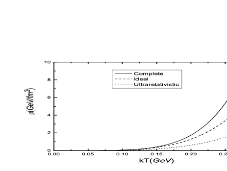
Figure 1: Plot of the energy density $\rho$ in $GeV/fm^{3}$ as a function of the thermal energy $kT$ given in $GeV$. Three curves are presented: the complete energy density which includes the effects of all the relevant particles and their interactions (full line); energy density of all particles (ultrarelativistic, relativistic and hadronic) without considering interactions, i.e., all the particles are taken as ideal ones (dashed line); energy density for the ultrarelativistic particles (dotted line).

The complete EOS for the pressure $p$ comes from the substitution of Eqs.( 27), (4) and (32) into (24). Figure 2 shows the plot of function $p=p(kT)$.

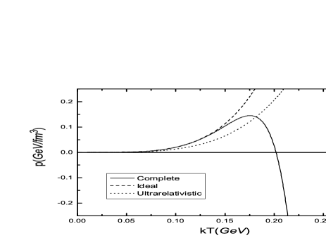
Figure 2: Plot of the pressure $p$ in $GeV/fm^{3}$ as a function of the energy $kT$ given in $GeV$. Interactions are accounted for only in the complete case (full line). The conclusion is: interaction drags the pressure to negative values, pointing to cosmic acceleration.

It can be seen in Figure 2 that, up to $0.14$ $GeV$, the three curves for the pressure present similar behavior: as in the energy density case, all are positive–valued and increase monotonically. From this point on the interaction contributions grow, and there is a sudden change in the slope for the complete system. The curve mitigates its increase rate, reaches a maximum at $0.175$ $GeV$, and then starts a steep fall. It becomes negative at around $0.2$ $GeV$ and continues to decrease at a high rate. A comparative graphic analysis of the effects on $\rho$ and $p$ coming from the different kinds of interactions and scatterings reveals that the relevant processes for the determination of $b_{2}$ in scales of $kT\lesssim 300$ $MeV$ are the scatterings $\pi\pi$, $\pi K$ and $\pi N$ related to the $S$ and $P$ partial waves. Therefore, it is fair enough to take into account only $l=0,1$ and $2$ when calculating $b_{2}$, just as we did.

A last point we would like to discuss is the validity range of the expansions $\rho(kT)$ and $p(kT)$. This validity is threatened by three factors: (I) an eventual phase transition due to instabilities in the function $p(kT)$; (II) the non-convergence of the pressure and energy density series, which would not allow the perturbative approach adopted here; (III) the occurrence of the deconfinement of hadrons in quarks and gluons, which would change the nature of the particles. Let us comment on these issues:

(I) There are two necessary and sufficient conditions that assure the stability of the usual thermodynamical systems Callen , namely:

$$\frac{1}{T}\left(\frac{\partial\rho}{\partial T}\right)_{n_{i}}\geq 0\text{ \ \ \ and \ \ \ }n_{i}\left(\frac{\partial p}{\partial n_{i}}\right)_{T}\geq 0\,,$$ (33)

with $i=\pi$, $K$, $N$ or $\mu$.

The function $\rho$ depends only on $kT$ ($z_{i}=1$ for every species $i$), while $p$ depends on $kT$ and also on the densities $n_{i}$ of the four types of particles. Thus, the second condition in (33) splits into four others, all required to guarantee the system stability. From Figure 1, it is easily seen that the curve $\rho(kT,\{z_{i}\})$ for the complete set always satisfies (33).

Notwithstanding, the same does not occur with $p\left(kT,\{n_{i}\}\right)$. Indeed, as the numerical densities are positive and increasing functions of $kT$, Figure 2 makes clear that the pressure does not obey condition (33); i.e., for some energy value higher than $0.14$ $GeV$ the EOS for the pressure becomes unstable. In principle, this instability is a strong indication of a phase transition and points to a breakdown of the EOS validity. However, this argument is based on the usual situation of a thermodynamical system: a gas confined in a recipient of finite volume. By its very nature, the universe cannot be assumed to have the same characteristics of such a simple and controlled environment. First: the universe has no frontiers. In this case, the surface pressure (which is different from the internal pressure) does not exists. And in many cases are precisely the surface effects which generate the phase transitions in an ordinary thermodynamical system. Second: in the context of cosmology, the (internal) pressure is a direct source of the gravitational field artigo 1 . This particular feature produces rather different effects from those engendered by the pressure in usual thermal systems, for which one would expect the reduction in the volume as the internal pressure increases. This notion, spelled by the second relation in (33), is of great importance, since it prevents the ordinary system from disappearing: if $\partial p/\partial V$ were positive, nothing would avoid the collapse of the gas. On the other hand, in the context of cosmology, an increase of pressure increases the gravitational attractive effect, and in this sense, a cosmological system with $\partial p/\partial V<0$ is unstable, i.e., if the universe is not expanding it tends to collapse. We want to emphasize the distinction between the effects of the internal pressure in the two types of systems: in ordinary equilibrium thermodynamics, an increase of $p$ leads to an increase of the volume $V$ of the recipient containing the gas because the shocks of the particles against the walls are more and more frequent; but in cosmology the increase of $p$ strengthens the gravitational field and produces a net tendency to the reduction of the volume. Hence, it is reasonable to say that the stability criterion (33) cannot be directly applied in cosmology, and cannot be used to rule out the above EOS. From the microscopic point of view, the energy density fluctuations $\delta\rho$ grow fast in regions where $\partial p/\partial\rho\equiv c_{s}^{2}<0$ ($c_{s}$ is named the sound velocity in the media) and the system becomes unstable. For the usual thermodynamical systems this strongly suggests phase transition. Our system, the standard cosmological model, is not of this type, though. The universe expands in a rate determined by the relation between $p$ and $\rho$. This complicates the analyzes and we can not affirm that $c_{s}^{2}<0$ necessarily leads to a phase transition of the system. The correct treatment of the evolution of $\delta\rho$ should be done along with the perturbations in the space-time geometry – FRW metrics. We leave these investigations for the future.

(II) The convergence of the expansions for $p$ and $\rho$ is related with the formal aspect of validity of these series and the correction of the perturbative treatment. This issue is far from trivial, since is not possible to sum all the terms for any realistic system in a pure thermodynamical context, let alone in the cosmological framework. The virial coefficients $a$, or the cluster integrals $b$, depend on the sum of the connected diagrams representing mutual interactions. And it is extremely difficult to foresee the behavior of the result when $N$ particles interact. So, the answer to the question concerning the convergence of $p$ and $\rho$ is inaccessible. Nevertheless, the authors proposed elsewhere artigo 1 a toy-model for the interactions in the early universe, computed the perturbed EOS (until third order) and showed that there is a good indication of convergence for the pressure series. So, we will assume in this work the validity of truncating the equations for $p$, $\rho$ and $n$ in the second order terms.

(III) The QCD coupling constant diminishes as the energy $kT$ increases. So, one could expect that at a certain critical temperature $kT_{c}$, its value becomes sufficiently low to allow for the deconfinement of the hadronic matter, giving rise to a system composed by quarks and gluons. If such a transition takes place during the PNS, our model ceases to be valid beyond $kT_{c}$: the EOS have been calculated assuming that the fundamental particles are hadrons, not quarks and gluons. According to the lattice QCD calculations Lattice , the critical temperature is situated between $150$ and $180$ $MeV$. From an experimental perspective, recent results from the RHIC RHIC indicate that a sort of transition occurs at these temperature, but it is not the deconfinement in a quark-gluon plasma QGP . The experiments run in RHIC found what seems to be a new state for the nuclear matter. This state would correspond to a perfect fluid (without viscosity) identified as a CGC (Color Glass Condensate) CGC . Unlike the quark-gluon plasma, the CGC has non negligible correlations, i.e., the nuclear interaction processes are relevant.

There is no doubt left by the experiments that the hadronic matter in the heavy ion colliders undergoes a phase transition in energies around $170$ $MeV$. But it is possible that this phenomenon does not occur in the primordial universe (or that it occurs in different energy scales), due to the various differences between the laboratory and the early universe. Specifically, the temporal scale of the events in the possible cosmological QCD transition ($10^{-5}s$) is quite different from the scale of the transition in the accelerators ($10^{-23}s$) Vega . Other differences – previously cited – are the non-existence of border in the cosmological system and the role of pressure as direct source of gravitation. It may happen that the new state of nuclear matter (CGC) discovered in RHIC is affected by the absence of borders or by the expansion of the universe. Even though we do not have strong arguments against the cosmological QCD transition, we will assume the hypothesis that it does not occur in the PNS period.

V Cosmological consequences

Let us admit that the proposed EOS, Eqs. (24) and (25), are valid during all the PNS period. A first application to cosmology can done through the usual parametrization

$$p(kT)=\omega(kT)\rho(kT).$$ (34)

Substituting (34) into the second Friedmann equation (2), and neglecting $\Lambda$, we find

$$\left(\frac{\ddot{a}}{a}\right)=-\,\frac{4\pi G}{3}\left[1+3\omega(kT)\right]\rho(kT).$$ (35)

As the energy density is a positive and increasing function of $kT$, the information about the acceleration rate depends on the parametric function $\omega(kT)$ solely. Isolating this quantity in (34) and using the explicit forms of $\rho(kT)$ and $p(kT)$, the plot of Figure 3 obtains.

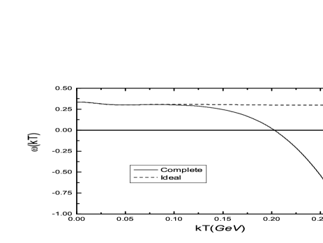
Figure 3: Plot of $\omega$ as a function of $kT$. Two curves are shown: the complete $\omega$ function, including all the particles and relevant interactions (full line); ideal $\omega$ function, which computes all the particles but not the mutual interactions (dashed line).

It shows that the complete and the ideal curves for $\omega$ are practically superimposed until $0.11$ $GeV$. From this value on, the complete $\omega$ curve begins to decrease, becoming negative at about $0.2$ $GeV$. On the other hand, the ideal $\omega$ curve remains positive and nearly constant up to $0.3$ $GeV$. The effect of the behavior of the complete $\omega$ function on (35) is to change the universe’s expansion rate between $0.1$ $GeV<kT<0.3$ $GeV$. As we go back in time, the universe passes continuously from a decelerated dynamics (pretty close to a radiation dominated era) to an accelerated stage. Comparison of the two lines in Figure 3 shows that this acceleration is due to the hadronic interaction processes.

The next step is to determine the scale factor $a(kT)$ and the function $t(kT)$ associating cosmic time and temperature (or thermal energy). We shall use the conservation equation,

$$\frac{d\rho}{da}=-\frac{3}{a}(p+\rho),$$ (36)

and the first Friedmann equation (2). We obtain $a(kT)$ by integrating (36):

$$a(kT)=a_{Pns0}\exp\left[-\int\limits_{kT_{Pns0}}^{kT}\frac{\frac{d\rho}{d\left(kT^{\prime}\right)}}{3(p+\rho)}d\left(kT^{\prime}\right)\right],$$ (37)

where the label $Pns0$ indicates that the quantity is calculated at the end of the pre-nucleosynthesis period which, in energy, is $kT_{Pns0}=20MeV$. The time function $t(kT)$ is obtained by the combination of (36) and (2) ($c$ is re-inserted):

$$t_{Pns0}-t=\int\limits_{kT_{Pns0}}^{kT}\frac{\frac{d\rho}{d\left(kT^{\prime}\right)}}{3(p+\rho)\sqrt{\frac{8\pi G}{3c^{2}}\rho-\frac{\kappa c^{2}}{a^{2}}}}d\left(kT^{\prime}\right)\text{,\ \ \ \ \ }\frac{8\pi G}{3c^{2}}=\frac{996\text{ }fm^{3}}{(ms)^{2}GeV}\,\,\,.$$ (38)

Equations (37) and (38) describe the evolution of the pre-nucleosynthesis universe. A careful analysis of these equations reveals that both diverge when $p=-\,\rho$ and, according to the complete EOS (with interactions included), this happens at $kT_{c}\simeq 0.2767$ $GeV$ (critical temperature). The scale factor always decreases as $kT$ increases. The decreasing rate $\frac{da}{d\left(kT\right)}$ is not so well-behaved: it varies a lot and, as $kT$ approaches $kT_{c}$, $\frac{da}{d\left(kT\right)}\rightarrow-\infty$. This means that the scale factor tends to zero when $kT\rightarrow kT_{c}$. In order to study the time function around $kT_{c}$ we have to particularize for the three values of $\kappa$:

1. For $\kappa=0$, the time interval $\left|t_{Pns0}-t_{c}\right|\rightarrow\infty$ when $kT\rightarrow kT_{c}$, because $\rho(kT)$ and $\frac{d\rho}{d\left(kT\right)}$ are always positive. In a plane space-section universe, the time interval that would elapse from the initial singularity till $t_{Pns0}$ is infinity, and that singularity is never attained.

2. For $\kappa=1$, we see from (2) that it exists a value of $kT$ close to $kT_{c}$ where $\dot{a}=0$. This value, indicated by $kT_{B}$, is close to $kT_{c}$ to $39$ decimal digits. Defining $a_{0}$ as the present–day value of the scale factor, and $a_{B}=a(kT_{B})$ as the minimum value of the scale factor, then it is found that $a_{B}\simeq 1.7\times 10^{-24}a_{0}$. Thus, in an universe of spherical space-section, the initial singularity does not exist; the universe reaches a minimum size measured by $a_{B}$. Recall that recent cosmological data PDG slightly favor $\kappa=1$ (as $\Omega_{T0}\simeq 1.003$). Combining this type of solution that presents a minimum size to the requirement that the closed model presents also a maximum size, we obtain the so called eternal universe, or bouncing universe Boucing . The time interval from the minimum radius till the end of the PNS period is determined by using (38) and the values of $H_{0}$ and $\Omega_{T0}$; it is $\left|t_{Pns0}-t_{B}\right|\simeq 2.28$ $ms$.

3. For $\kappa=-1$, the time interval $\left|t_{Pns0}-t_{c}\right|\rightarrow 2.28$ $ms$ when $kT\rightarrow kT_{c}$. Therefore, for a hyperbolic space-section, the initial singularity is reached in a finite time.

Notice that despite the different possible evolutions, the universe always presents a maximum temperature $kT_{c}$.

The statistical bootstrap model by Hagedorn also predicts a maximum temperature $kT_{H}$ for the universe; but the mechanisms that lead to it are distinct from the causes for our critical temperature $kT_{c}$. In the context of Hagedorn’s model, the increase in the total energy $E$ is responsible for the rise in the kinetic energy and also for the increase in the number of kinds of particles in the system. As $E$ rises it is more advantageous to produce new particles than to increase the temperature of the system. This ultimately results in an infinite limit for the energy ($E\rightarrow\infty$) and the pressure ($p\rightarrow\infty$) at a finite value of the temperature ($kT_{H}<\infty$). On the other hand, $kT_{c}$ is the temperature associated to the equality $p=-\,\rho$ in our cosmological model with interacting particles – see comments below Eq. (38); $kT_{c}$ appears due to the structure of the equations (2) and (36).

V.1 The inflationary regime

Function $\omega(kT)$ evolves continuously from $1/3$ (radiation era; $kT\leq 0.02$ $GeV$) and tends to $-1$ (as $kT\rightarrow kT_{c}$). The inflationary regime (primeval accelerated expansion period) occurs when $\omega(kT)<-1/3$. On the other hand, our model requires that $\omega(kT)>-1$. We match these requirements by defining the inflationary period as that for which $-1<\omega(kT)<-\frac{1}{3}$. According to Figure 3, this corresponds to the energy interval

$$0.2356\text{ }GeV\simeq kT_{accel}<kT<kT_{c}\simeq 0.2767GeV.$$ (39)

An early acceleration is required to solve some cosmological problems – horizon, flatness, origin of the inhomogeneities, etc. – without imposing specific initial conditions Guth ; kolb ; Liddle . An accelerated regime, however, must exhibit some special features to actually rule out these problems. We now show that our model indeed eliminates the horizon and flatness problems.

The horizon problem is the lack of causal connection between regions far apart which nevertheless exhibit similar physical characteristics. The region of causal connection is quantified by the Hubble radius $R\equiv(aH)^{-1}$, the maximal distance particles can travel during an $e$-fold increase of the scale factor, an increase by the factor $e\simeq 2.78$ Dod . The standard Bib Bang model tells us that, from the time $t_{Pns0}$ until the present day, the maximum commoving distance between two causal connected regions grew $9$ orders of magnitude:

$$\frac{R_{0}}{R_{Pns0}}=\frac{a_{Pns0}H_{Pns0}}{a_{0}H_{0}}\sim 1.4\times 10^{9}.$$ (40)

Let $kT_{hor}$ be the energy value above which all the universe’s content is in causal contact. In order to solve the horizon problem in the context of our model, we need to show that there is a $kT_{hor}<kT_{c}$ such that

$$\frac{R_{Pns0}}{R_{hor}}=\frac{a\left(kT_{hor}\right)H(kT_{hor})}{a_{Pns0}H_{Pns0}}\sim 7.2\times 10^{-10}.$$ (41)

This is done by using Eqs.(2) and (37). Indeed, for all the values of $\kappa$, the $kT_{hor}$ satisfying (41) respects $\left(kT_{c}-kT_{hor}\right)\simeq 10^{-35}$.

Analysis of the Hubble radius shows that, from the beginning of the deceleration ($kT_{accel}\simeq 0.2356$ $GeV$) till nowadays, $R$ has increased $1.75\times 10^{10}$. But from $kT_{hor}$ to $kT_{accel}$ the Hubble radius diminished $1.8\times 10^{10}$. And for values of time smaller than that corresponding to $kT_{hor}$ all the universe was in causal contact, allowing the thermalization of the cosmic fluid.

The flatness problem may be treated quantitatively through the first Friedmann equation

$$1-\Omega_{T}=-\frac{\kappa c^{2}}{a^{2}H^{2}}=\Omega_{\kappa},\text{\ \ \ \ \ }\Omega_{T}\equiv\frac{\rho}{\rho_{c}}\equiv\frac{8\pi G\rho}{3c^{2}H^{2}}.$$ (42)

According to recent data $\Omega_{T0}\simeq 1.003$. Now, $aH$ decreases with time if the universe is of the radiation-dominated or matter-dominated types (the usual cases). This means that $\left|\Omega_{\kappa}\right|$ increases with time in radiation and matter-dominated models. If this is so, in the early universe $\left|\Omega_{\kappa}\right|\ll$ $10^{-3}$ and we are led to the question: Why was the total density value $\rho$ so close to the critical density $\rho_{c}$ in the initial instants of the universe when $\kappa=\pm 1$? This necessary fine-tuning in the initial condition for $\rho$ is the flatness problem.

The standard model establishes that the energy density at the end of the pre-nucleosynthesis period $\rho_{Pns0}$ is close to $\rho_{c}$ within a precision of $21$ decimal digits. Hence, to solve the flatness problem one needs to show that there is a value $kT_{flat}<kT_{c}$ such that

$$\left|\Omega_{\kappa}\right|_{flat}=\frac{1.5\times 10^{-21}a_{Pns0}^{2}H_{Pns0}^{2}}{a^{2}(kT_{flat})H^{2}(kT_{flat})}\sim 10^{-3}.$$ (43)

The value $kT_{flat}$ verifying (43) is found to be $\left(kT_{c}-kT_{flat}\right)\simeq 10^{-35}$ (for $\kappa=\pm 1$). From $kT_{flat}$ to the end of the PNS, the scale factor increases $12$ orders of magnitude. And this large variation happens in a time interval of $2.25$ $ms$, by Eq. (38). The duration of the accelerated expansion is much smaller: $0.26$ $ms$. This makes clear that the high inflationary rate – $a(kT)$ increase of $10$ orders of magnitude in $0.26$ $ms$ – rapidly flattens the universe.

The values (of the thermal energy, of the scale factor) characterizing the PNS period in what concerns the inflationary issues are collected in Table 1.

$$\Delta t(ms)$$

Table 1: Resumé of the main results concerning the behavior of our model in the PNS period and the accelerated regime. $kT_{Pns0}=0.020$ $GeV$ is the temperature at the end of the PNS; $kT_{acel}$ is the temperature below which there is no acceleration; $kT_{hor}$ is the temperature at which the causality problem is solved; and $kT_{flat}$ is the temperature that rules out the fine-tuning in $\rho$. Definitions: $\Delta t=t_{Pns0}-t$ and $a_{Pns0}\equiv 1$.

VI Final remarks

This work presents equations of state (EOS) for the early universe which include the interactions among the constituent particles. We argue that the dominant processes affecting the pre-nucleosyntesis period (PNS) are those involving the strong interaction, the only which has been considered. Total EOS accounting for photons, leptons and hadrons have been built, using a phenomenological description of the hadronic interaction and assuming thermodynamical equilibrium. Assuming the hypothesis of no deconfinement, some interesting points have turned up.

First, the interactions naturally drove the pressure to negative values. The de Sitter model has taught us long ago that an exotic equation of state, $p=-\rho$, in which the pressure is negative, would give rise to an accelerated expanding universe. Therefore, our results could explain the primeval acceleration regime, as an alternative scenario to (scalar field) inflation. Indeed, our model is able to connect this initial accelerated stage with a decelerated expansion of the type expected for a radiation-dominated universe. In addition, the acceleration generated in our interacting cosmic fluid has been shown to be intense enough to solve the horizon and flatness problems.

Another noticeable feature has been obtained: for the models with $\kappa=0$ or $\kappa=1$ the initial singularity is avoided, and a natural explanation for the expansion of the universe emerges. In fact, either in an eternal universe (compatible with $\kappa=1$) or in a universe with a beginning (corresponding to $\kappa=0$), the primeval acceleration produced by the strong interaction is capable of engendering an expansion which evolves to a decelerated type and continue its dynamics. Nevertheless, let us emphasize that these results have been derived for a symmetric universe: the quantity of matter is assumed to equal that of antimatter.

Such effects are actually more general than the results of the specific model proposed. Indeed, in order for then to be valid it is enough to introduce in the FRW cosmology a continuous parameter $\lambda$ (related or not to interactions) responsible for the passage from $p(\lambda)=\frac{\rho(\lambda)}{3}$ to the exotic EOS    $p(\lambda)=-\rho(\lambda)$ in such a way that $\frac{d\rho}{d\lambda}>0$ at all times. This type of fitting links smoothly the accelerated and decelerated expansion periods via the parametric equation $p=\omega\rho$ in which $\omega$ varies between $1/3$ and $-1$. This interval automatically eliminates the ghost models($\omega\leq-1$) ghost .

Besides the mechanisms engendering primeval acceleration, there are other important subjects related to the pre-nucleosynthesis period to be discussed. Amongst them, we highlight two: the generation of the initial perturbations of the energy density content and the matter-antimatter asymmetry. The initial perturbations might be generated in the context of our model through the introduction of statistical fluctuation processes mag ; this possibility shall be investigated in the future. The problem of the matter-antimatter asymmetry is more involved: as it is well known, the inflation wipes out all the traces of an eventual initial asymmetry and this demands the existence of a mechanism driving a post-inflationary matter-antimatter asymmetry. Moreover, a necessary condition to produce an excess of particles over anti-particles is the system to be out of the thermodynamical equilibrium Sak . This exigence prevents our model to describe this asymmetry once all the numerical densities are obtained from the statistical mechanics in thermal equilibrium. This limitation could be overcome if we consider out-of-equilibrium phase-transition in a post-inflationary stage. A mechanism of this kind was proposed in Ref. ucrafour and will the investigated in another opportunity.

From a wider perspective, this works calls attention to the fact that particle interactions are a direct source of gravitation artigo 1 . When one ignores this truth, simplifications result in the cosmological models; but these are perhaps too large to enable a proper description of the real universe. The role of the fundamental interactions in cosmology opens new paths to the study of the universe evolution, and even if our complete EOS are not valid during all the PNS period, the central idea may be applied to model other eras. Up to this point, we would not dare to affirm that the inclusion of hadronic interactions is more appropriated than the scalar fields to generate the inflation. Many issues solved by the inflationary theory have been left untouched here. But the interaction scheme is certainly more suitable from the theoretical point of view: they have a clear physical interpretation.

Appendix A Multi-component systems

A multi-component system is a set with more than one type of particle or conserved quantum number. The grand canonical partition function $\Theta$ for a $B$-components system is, in analogy to (9),

$$\Theta(z_{1},..,z_{B},V,T)=\sum\limits_{N_{1}=0}^{\infty}...\sum\limits_{N_{B}=0}^{\infty}Q_{N_{1},...,N_{B}}(V,T)z_{1}^{N_{1}}...z_{B}^{N_{B}}.$$ (44)

(See Refs. Smith Lain 81 ; Osborn 77 .) The grand canonical potential $\Omega$ as a function of the fugacities (and the temperature) is, then,

$$\Omega(z_{1},...,z_{B},T)=\frac{1}{V}\ln\Theta(z_{1},...,z_{B},V,T)=\sum\limits_{N_{1}=0}^{\infty}...\sum\limits_{N_{B}=0}^{\infty}b_{N_{1},...,N_{B}}z_{1}^{N_{1}}..z_{B}^{N_{B}},$$ (45)

where $b_{N_{1},...,N_{B}}$ are the $B$-component cluster integrals, with $b_{0,...,0}\equiv 0$ ($N_{1}=N_{2}=...=N_{B}=0$).

The construction of the equations of state – pressure $p=p(z_{1},..,z_{B},T)$, energy density $\rho=\rho(z_{1},..,z_{B},T)$ and numerical densities $n_{1}(z_{1},..,z_{B},T)$, $n_{2}(z_{1},..,z_{B},T)$,…, $n_{B}(z_{1},..,z_{B},T)$ – is done through the usual mapping from statistical mechanics to thermodynamics, namely

$$\frac{p(z_{1},...,z_{B},T)}{kT} \equiv\Omega=\sum\limits_{N_{1}=0}^{\infty}...\sum\limits_{N_{B}=0}^{\infty}b_{N_{1},...,N_{B}}z_{1}^{N_{1}}...z_{B}^{N_{B}},$$ (46a)

$$n_{i}(z_{1},...,z_{B},T) \equiv z_{i}\left(\frac{\partial\Omega}{\partial z_{i}}\right)_{V,T,\left\{z_{B}\right\}\neq z_{i}}=\sum\limits_{N_{1}=0}^{\infty}...\sum\limits_{N_{B}=0}^{\infty}N_{i}b_{N_{1},...,N_{B}}z_{1}^{N_{1}}...z_{B}^{N_{B}},$$ (46b)

$$\rho(z_{1},...,z_{B},T) \equiv kT^{2}\left(\frac{\partial\Omega}{\partial T}\right)_{V,\left\{z_{B}\right\}}=\left(kT\right)^{2}\sum\limits_{N_{1}=0}^{\infty}...\sum\limits_{N_{B}=0}^{\infty}\frac{\partial b_{N_{1},...,N_{B}}}{\partial\left(kT\right)}z_{1}^{N_{1}}...z_{B}^{N_{B}}.$$ (46c)

Symbol $$\left\{z_{B}\right\} z_{1} z_{B}$$ is the set of fugacities, from to . As in the one-component case, these is another form for the EOS: that corresponding to the virial expansion, with the pressure and the energy density in terms of the numerical densities. It is:

$$\frac{p(n_{1},...,n_{B},T)}{kT}=\sum\limits_{l_{1}=0}^{\infty}...\sum\limits_{l_{B}=0}^{\infty}a_{l_{1},...,l_{B}}(T)n_{1}^{l_{1}}...n_{B}^{l_{B}},$$ (47a)

$$\frac{\rho(n_{1},...,n_{B},T)}{\left(kT\right)^{2}}=\sum\limits_{l_{1}=0}^{\infty}...\sum\limits_{l_{B}=0}^{\infty}c_{l_{1},...,l_{B}}(T)n_{1}^{l_{1}}...n_{B}^{l_{B}}.$$ (47b)

The virial coefficients $$a_{l_{1},...,l_{B}} c_{l_{1},...,l_{B}} b_{N_{1},...,N_{B}}$$ and are determined by the clusters integrals . For a 2-component case, the first virial coefficients are

$$\left.a_{0,0}=0,\text{\ \ \ \ \ \ \ }a_{0,1}=a_{1,0}=1,\right.$$ (48a)

$$\left.a_{2,0}=\frac{-b_{2,0}}{b_{1,0}^{2}},\text{\ \ }a_{0,2}=\frac{-b_{0,2}}{b_{0,1}^{2}},\text{\ \ }a_{1,1}=\frac{-b_{1,1}}{b_{1,0}b_{0,1}},\right.\text{\ }$$ (48b)

$$\left.c_{0,0}=0,\text{\ \ \ \ \ }c_{1,0}=\frac{\dot{b}_{1,0}}{b_{1,0}},\text{\ \ }c_{0,1}=\frac{\dot{b}_{0,1}}{b_{0,1}},\right.$$ (49a)

$$\left.c_{2,0}=-\dot{a}_{2,0},\text{\ \ }c_{0,2}=-\dot{a}_{0,2},\text{\ \ }c_{1,1}=-\dot{a}_{1,1}.\right.$$ (49b)

The dot ^⋅ indicates differentiation with respect to $$kT$$. Equation (22) for a 2-component system reads:

$$b_{2,0}-b_{2,0}^{(0)} = \frac{1}{2\beta\pi^{3}}\sum\limits_{a}\sum\limits_{l=0}^{\infty}g_{2,0}^{a}\left(2l+1\right)\int\limits_{2m_{X}}^{\infty}\omega^{2}K_{2}(\beta\omega)\left[\frac{\partial\delta_{l}^{a}(\omega)}{\partial\omega}\right]_{2,0}d\omega,$$ (50a)

$$b_{0,2}-b_{0,2}^{(0)} = \frac{1}{2\beta\pi^{3}}\sum\limits_{a}\sum\limits_{l=0}^{\infty}g_{0,2}^{a}\left(2l+1\right)\int\limits_{2m_{Y}}^{\infty}\omega^{2}K_{2}(\beta\omega)\left[\frac{\partial\delta_{l}^{a}(\omega)}{\partial\omega}\right]_{0,2}d\omega,$$ (50b)

$$b_{1,1}-b_{1,1}^{(0)} = \frac{1}{2\beta\pi^{3}}\sum\limits_{a}\sum\limits_{l=0}^{\infty}g_{1,1}^{a}\left(2l+1\right)\int\limits_{m_{X}+m_{Y}}^{\infty}\omega^{2}K_{2}(\beta\omega)\left[\frac{\partial\delta_{l}^{a}(\omega)}{\partial\omega}\right]_{1,1}d\omega,$$ (50c)

where $$m_{X} m_{Y}$$ and are the masses of the first and second components. The ideal terms are determined from the free-system Ruben1 as:

$$b_{1,0} =\frac{g_{X}}{\Lambda_{X}^{3}(\beta)},\text{\ \ \ \ }b_{0,1}=\frac{g_{Y}}{\Lambda_{Y}^{3}(\beta)},\text{\ \ \ \ }b_{1,1}^{(0)}=0~{};$$ (51a)

$$b_{2,0}^{(0)} =\frac{(\pm 1)g_{X}}{2\Lambda_{X}^{3}(2\beta)},\text{\ \ }b_{0,2}^{(0)}=\frac{(\pm 1)g_{Y}}{2\Lambda_{Y}^{3}(2\beta)},$$ (51b)

where $$g_{X} g_{Y} \Lambda(j\beta)$$ and are the number of internal degrees of freedom of the free-systems; the upper (lower) signs refer to the Bose-Einstein (Fermi-Dirac) statistics; and, is the relativistic thermal wave-length

$$\Lambda_{X,Y}^{3}(j\beta)=\frac{\left(2\pi\right)^{3}j\beta}{4\pi m_{X,Y}^{2}K_{2}(j\beta m_{X,Y})}.$$ (52)

The generalization for more than two components is straightforward.

Appendix B Hadronic scattering

Elastic hadronic scattering processes can be described by the phase shifts $\delta$ in the context of the partial–wave formalism. In this approach, one uses the spectroscopic classification and separates the “elastic” process involving interactions among pions, kaons and nucleons in six types. They are: $\pi\pi$, $\pi K$, $\pi N$, $KK$, $KN$ and $NN$. There is a set of phase shifts $\delta$ for each of such processes. The $\delta$’s are directly or indirectly determined from the experimental data. We will discuss in detail how this is done in the case of the pion-pion scattering.

The “elastic” pion-pion scattering depends on the energy, the total orbital angular momentum $L$ and the total isospin $I$. It is then convenient to introduce the notation $\delta_{L,I}$ for each phase shift. As a scattering of identical particles with integral spin, the associated two-pions total state (orbital angular momentum state plus isospin state) must be symmetric. We will take $I=0$, $1$, $2$ and restrict the analyses to $L=0$, $1$, $2$ (partial waves $S$, $P$ and $D$). This restriction is not arbitrary: it is imposed by the experimental data that are available. Hence, the relevant phase shifts are those in Table B.1.

$$S\text{-Wave}$$

Table B.1: Phase shifts $\delta_{L,I}$ for $\pi\pi$-scattering. The degeneracy degree $g$ accounts for the bosonic symmetry and the projections of orbital angular momentum $\left(2L+1\right)$ and of isospin $\left(2I+1\right)$.

The data for the phase shifts $\delta_{0,0}$ and $\delta_{1,1}$ are found in Ref. EstaMartin ; Rosselet , which give the results for the extensively repeated and measured scattering $\pi^{-}p\rightarrow\pi^{-}\pi^{+}n$. The data for $\delta_{0,2}$, $\delta_{2,0}$ and $\delta_{2,2}$ EstaMartin ; FrogPeter are determined through modeling based on the Roy equation Roy ; Basdevant . The $S$-wave data are shown in Figure 4.

Figure 4: Experimental data for the $S$-wave $\pi\pi$ scattering and the corresponding fitted curves for the functions $\delta_{L,I}\left(\omega\right)$.

The fits for each one of the phase shifts were done using the software Origin $6.1$ via the polynomial regression method or the non-linear least squares fitting. The experimental uncertainties were considered. The best-fit phase shifts are given by the expressions

$$\delta_{0,0}\left(\omega\right)=-1.13+4.36\omega-0.11\omega^{2}-4.52\omega^{3}+3.76\omega^{4},$$ (53)

and

$$\delta_{0,2}\left(\omega\right)=-0.03+1.23\omega-6.67\omega^{2}+12.62\omega^{3}-13.39\omega^{4}+8.57\omega^{5}-3.11\omega^{6}+0.48\omega^{7}.$$ (54)

Analogously, we can obtain the fitted curves $\delta_{L,I}=\delta_{L,I}\left(\omega\right)$ for partial waves $P$ and $D$. The functions $\delta_{L,I}\left(\omega\right)$ – such as (53) and (54) – are differentiated with respect to the energy and substituted in equations (50a-50c) for the cluster integrals $b$ which, in turn, are used to obtain the $p$ and $\rho$ equations of state for the PNS universe.

The other scatterings ($\pi K$, $\pi N$, $KK$, $KN$ and $NN$) are treated in the same way. The experimental data used in the description of the pion-kaon scattering are found in Ref. EstaCarnegie and they are good enough only to analyze the values $L=0$, $1$ – $S$-waves and $P$-waves. In the case of the pion-nucleon scattering, the relevant reference is CNS and we study $L=0$, $1$, $2$ ($S$, $P$ and $D$-waves). The kaon-kaon scattering data are (indirectly) obtained from FrogPeter ; KamiLesnLois and FurnLesn  using the separable potential formalism ActaPolonia ; KamiLesn ; these data refer solely to the $S$-wave $K\bar{K}$ scattering (we suppose that the processes $K\bar{K}$ and $KK$ are identical, which means that the processes are independent of charge conjugation $C$. The kaon-nucleon phase shifts (for $S$, $P$ and $D$-waves) are in Ref. CNS – once again we admit independence under $C$. The same Ref. CNS presents the nucleon-nucleon data for $S$, $P$ and $D$-waves and, in these cases, in addition to the $C$-independence, it is assumed independence on the isospin $I$: the proton-proton phase shifts are very similar to the neutron-neutron ones.

References

- (1) V. Narlikar, Introduction to Cosmology, 2nd ed., Cambridge University Press, 1993.
- (2) S. Weinberg, Gravitation and Cosmology. Principles and Aplications of the General Theory of Relativity, John Wiley and Sons, New York, 1972.
- (3) R. Aldrovandi, R. R. Cuzinatto and L. G. Medeiros, Foundations of Physics 36, 1736 (2006); [gr-qc/0508073].
- (4) S. Dodelson, Modern Cosmology: Anisotropies and Inhomogeneities in the Universe, Academic Press, 2003.
- (5) E. W. Kolb and M. S. Turner, The Early Universe, Perseus Books, 1994.
- (6) D. N. Spergel et. al., Astrophys. J. Suppl. 170 377 (2007); [astro-ph/0603449].
- (7) M. Colless et al., MNRAS, 328, 1039 (2001).
- (8) R. Aldrovandi, R. R. Cuzinatto, L. G. Medeiros, Interacting Constituents in Cosmology, to appear in Int. J. Mod. Phys. D; [gr-qc/0705.1369].
- (9) D. Rapetti, S. W. Allen, M. A. Amin, R. D. Blandford, Mon. No. Ro. Ast. Soc. 375, 1510 (2007); [astro-ph/0605683] – S. Permutter et al, Nature 391, 51 (1998); [astro-ph/ 9712212] – A. G. Riess et al., The Astronomical Journal 116, 1009 (1998); [astro-ph/9805201].
- (10) A. R. Liddle e D. H. Lyth, Cosmological Inflation and Large-Scale Structure, Cambridge University Press, 2000.
- (11) A. H. Guth, Phys. Rev. D23, 357 (1981).
- (12) A. Albrecht & P. J. Steinhardt, Phys. Rev. Lett. 48, 1220 (1982).
- (13) A. D. Linde, Phys. Lett. B108, 389 (1982).
- (14) R. R. Caldwell, R. Dave & P. J. Steinhardt, Phys. Rev. Lett. 80, 1582 (1998); [astro-ph/9708069].
- (15) P. J. Steinhardt, L. Wang & I. Zlatev, Phys. Rev. D59, 123504 (1999); [astro-ph/9812313].
- (16) P. J. Steinhardt, L. Wang & I. Zlatev, Phys. Rev. Lett. 82, 896 (1999); [astro-ph/9807002].
- (17) U. França & R. Rosenfeld, JHEP 210, 015 (2002); [astro-ph/0206194].
- (18) B. Ratra & P. J. E. Peebles, Phys. Rev. D37, 3406 (1988).
- (19) M.C. Bento, O. Bertolami, A.A. Sen, Phys. Rev. D66 043507 (2002); [gr-qc/0202064] – M.C. Bento, O. Bertolami, Anjan Ananda Sen; Phys. Rev. D70 083519 (2004); [astro-ph/0407239].
- (20) S. Capozziello, S. Carloni, A. Troisi, Recent Research Developments in Astronomy & Astrophysics - RSP/AA/21 (2003); [astro-ph/0303041] – S. Capozzielo et. al., Phys. Lett. A299, 494 (2002).
- (21) G. M. Kremer, Gen. Rel. Grav. 36, 1423 (2004); [gr-qc/0401060].
- (22) A. Brookfield, C. van de Bruck, D.F. Mota, D. Tocchini-Valentini, Phys. Rev. Lett. 96, 061301 (2006) and Phys. Rev. D73, 083515 (2006).
- (23) L. Amendola, G. C. Campos, R. Rosenfeld, Phys. Rev. D75, 083506 (2007); [ astro-ph/0610806].
- (24) N. Pinto-Neto, B. M. O. Fraga, to appear in General Relativity and Gravitation (2007); [gr-qc/0711.3602].
- (25) R. Dashen, S-K. Ma & J. Bernstein, Phys. Rev. 187, 345 (1969). Errata – Phys. Rev. A6, 851 (1972).
- (26) L. E. Reichl, A Modern Course in Statistical Physics, University of Texas Press, Austin, 1980.
- (27) R.K. Pathria, Statistical Mechanics, 2nd. ed., Butterworth Heinemann, Oxford, 1996.
- (28) E. Beth & G. E. Uhlenbeck, Physica 3, 729 (1936) e Physica 4, 915 (1937).
- (29) A. I Bugrii & A. A. Trushevskii, Astrophysics 13, 195 (1978).
- (30) A. I Bugrii & A. A. Trushevskii, Zh. Eksp. Teor. Fiz., 73, 3 (1977) – In Russian.
- (31) Y. U. Beletsky, A. I Bugrii & A. A. Trushevskii, Z. Phys. C10, 317 (1981).
- (32) Y. U. Beletsky, A. I Bugrii & A. A. Trushevskii, Astrophysics 24, 107 (1986).
- (33) R. Aldrovandi, J. P. Beltrán Almeida and J. G. Pereira, Int. J. Mod. Phys. D13 2241 (2004); [gr-qc/0405104].
- (34) J. E. Mayer, J. Chem. Phys. 5, 67; J. E. Mayer & P. G. Ackermann, J. Chem. Phys. 5, 74 (1937).
- (35) T. D. Lee & C. N. Yang, Phys. Rev. 113 1165; 116, 25 (1959).
- (36) D. Griffiths, Introduction to Elementary Particles, John Wiley & Sons, New York, 1987.
- (37) J. O. Hirschfelder, C. F. Curtiss & R. B. Bird, Molecular Theory of Gases and Liquids, John Wiley and Sons, New York, 1954.
- (38) P. Braun-Munzinger et al, Review for QGP3; [nucl-th/0304013].
- (39) A. Andronic et al, Nucl. Phys. A772, 167 (2006); [nucl-th/0511071]
- (40) A. Tawfik, Phys. Rev. D71, 54502 (2005); [hep-ph/0412336].
- (41) M. Cheng et al; [hep-lat/0710.0354].
- (42) G. D. Yen et al, Phys. Rev. C56, 2210 (1997); [nucl-th/9711062].
- (43) R. Hagedorn, Supp. Nuovo Cimento 3, 147 (1965).
- (44) W. Weinhold et al, Phys. Lett. B433, 236 (1998); [nucl-th/9710014].
- (45) H.B. Callen, Thermodynamics and an Introduction to Thermostatistics, 2d ed., John Wiley and Sons, New York, 1985.
- (46) F. Karsch, Nucl. Phys. A698, 199 (2002).
- (47) Relativistic Heavy Ion Collider, site - http://www.bnl.gov/rhic/.
- (48) D. H. Rischke, Progress in Particle and Nucl. Phys. 52, 197 (2004); [nucl-th/0305030].
- (49) E. Iancu & R. Venugopalan, Review for QGP3; [hep-ph/0303204].
- (50) D. Boyanovsky et al, Ann. Rev. Nucl. Part. Sci. 56, 441, (2006); [hep-ph/0602002].
- (51) Particle Data Group, site - http://pdg.lbl.gov/.
- (52) M. Novello, V Brazilian School of Cosmology and Gravitation, World Scientific, Cingapura (1987) – M. Novello, VII Brazilian School of Cosmology and Gravitation, Editions Frontières, Cingapura (1993) – M. Novello, J. M. Salim, The stability of a bouncing universe, (2003); [hep-th/0305254].
- (53) Sean M. Carroll, Mark Hoffman & Mark Trodden, Phys. Rev. D68, 023509 (2003); [astro-ph/0301273] – Robert R. Caldwell, Marc Kamionkowski & Nevin N. Weinberg, Phys. Rev. Lett. 91, 071301(2003); [astro-ph/0302506] – V. K. Onemli, R. P. Woodard, Phys. Rev. D70, 107301 (2004); [gr-qc/0406098].
- (54) J. Magueijo & L. Pogosian, Phys. Rev. D67, 043518 (2003); [astro-ph/0211337].
- (55) A. D. Sakharov, Soviet Physics Journal of Experimental and Theoretical Physics (JETP) 5 24 (1967).
- (56) C. R. Smith, R. Inguva & K. D. Lain, Phys. Rev. A23, 3285 (1981).
- (57) T. A. Osborn, Phys. Rev. A16, 334 (1977).
- (58) R. Aldrovandi, J. Gariel & G. Marcilhacy, On the pre-nucleosynthesis cosmological period, Rev. Ciöenc. Ex. Nat., 5 133 (2003); [gr-qc/0203079].
- (59) P. Estabrooks & A. D. Martin, Nucl. Phys. B79, 301 (1974).
- (60) L. Rosselet et al, Phys. Rev. D15, 574 (1977).
- (61) C. D. Froggatt & J. L. Petersen, Nucl. Phys. B129, 89 (1977).
- (62) P. Estabrooks et al, Nucl. Phys. B133, 490 (1978).
- (63) Center for Nuclear Studies (Said Program), site: http://gwdac.phys.gwu.edu/: online data.
- (64) L. Leśniak, Acta Physica Polonica B8, 1835 (1996).
- (65) R. Kamiński & L. Leśniak, Phys. Rev. D50, 3145 (1994).
- (66) R. Kamiński, L. Leśniak & B. Loiseau, Phys. Lett. B413, 130 (1997).
- (67) A. Furman & L. Leśniak, Phys. Lett. B538, 266 (2002).
- (68) S. M. Roy, Phys. Lett. B36, 353 (1971).
- (69) J. L. Basdevant, C. D. Froggatt & J. L. Petersen, Nucl. Phys. B72, 413 (1974).