JAGIELLONIAN UNIVERSITY
INSTITUTE OF PHYSICS
Proton induced spallation
reactions in the energy range
0.1 - 10 GeV
Anna Kowalczyk
![[Uncaptioned image]](/html/0801.0700/assets/x1.png)
A doctoral dissertation prepared at the Institute of Nuclear Physics of the Jagiellonian University, submitted to the Faculty of Physics, Astronomy and Applied Computer Science at the Jagiellonian University, conferred by Dr hab. Zbigniew Rudy
Cracow 2007
Chapter 1 Introduction
Several possible scenarios of proton - nucleus reaction are considered nowadays. According to one of the scenarios, incoming proton deposits energy into target nucleus. It knocks out a few nucleons and leaves excited residual nucleus. Then, nucleons and various fragments are emitted from the excited residuum. This scenario is called spallation. It is also possible, that the residuum splits up slowly (fissions) into two parts, which then emit particles. This scenario is known as emission from fission fragments. But, it could be also that all fragments appear simultaneously. This would have features of a phase transition in nuclear matter and is called fragmentation. These reaction scenarios are based on experimental observations of different final states. Generally, observation of one heavy nucleus (in respect to the mass of initial target), a small number of light fragments and numerous individual nucleons indicates spallation. Detection of a large number of intermediate size fragments indicates fragmentation. Nevertheless, spallation and fragmentation are correlated. Their differentiation is not clear, difficult and still under discussions. Previous studies indicate, that spallation is the most probable scenario of proton - nucleus reaction, what will be shown also in this dissertation. The main idea of this work concerns theoretical study of proton induced spallation reactions in wide range of incident energy and mass of target nuclei; fission and fragmentation are not discussed in details.
The following definition of spallation process can be found in Nuclear Physics
Academic press:
”Spallation - a type of nuclear reaction in which the high-energy of
incident particles causes the nucleus to eject more than tree
particles, thus changing both its mass number and its atomic number.”
So, the term spallation means a kind of nuclear reactions, where
hadron with high kinetic energy (100 MeV up to several GeV) interacts with
a target. First, this term was connected with observation of residuum of
reaction corresponding to losses of mass of target nucleus from few up to
several dozen nucleons.
Nowadays, it means mechanism, in which high energy light particle causes
production of numerous secondary particles from target nucleus, leaving cold
residuum of spallation. As a result of such process also various Intermediate
Mass Fragments (IMF), i.e. fragments with masses in range ,
are observed.
From historical point of view, the possibility of heating a nucleus via
bombarding by neutrons was suggested first time in 1936 by N. Bohr
[1].
Studies of similar reactions were possible due to development of accelerator
technics. It was in the end of fourties, when accelerators could provide
projectiles with energies higher than 100 MeV [2]. Experimentally,
two - component spectra of emitted particles are observed:
anisotropic high energy part, which dominates in forward angles
(i.e. the high energy tail
decreases at backward angles, as it is seen in the example Fig.
1.1) and isotropic, low energy part.

These general features of spallation process are established experimentally. A theoretical picture of an incident particle colliding successively with several nucleons inside target nucleus, losing a large fraction of its energy was proposed by Serber in 1947 [3]. Before, in 1937 Weisskopf considered possibility of emission of neutron from excited target nucleus [4]. In the end of fifties, Metropolis [5] and Dostrovsky [6] (who used the ideas of Serber and Weisskopf) suggested description of spallation as two step process involving energy deposition and subsequent evaporation. They formulated and performed first Monte Carlo calculations of the reactions. Such treatment of spallation reactions is used from that time up to now.
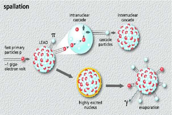
In more details, the first, so-called fast stage of the spallation is highly
non-equilibrated process. High energy proton causes an intra-nuclear
cascade on a time scale s. The incident projectile goes
through the target nucleus and deposits a significant amount of excitation
energy and angular momentum, while ejecting only a few high energy nucleons
and, with a minor yield, pions and light ions.
The result of the first stage is excited residual nucleus in thermodynamical
equilibrium (totally or partly equilibrated), with excitation energy
a few MeV/nucleon.
In case of thick target, i.e. system of several nuclei, the
ejectiles, as secondary projectiles can cause so-called inter-nuclear
cascade, placing individual nuclei into excited states,
as illustrated in Fig. 1.2.
The second, so-called slow stage of the spallation, consists in deexcitation of
the residuum by evaporation of particles.
The isotropic emission (in the system of nucleus) of nucleons
(mainly neutrons), light and heavy ions (d, t, He, Li, Be, B, …, )
takes place on a time scale - s.
From many years spallation reactions of medium and high energy protons with
atomic nuclei are still of interest for many reasons. First of all,
because knowledge of the reaction mechanism is still not complete.
This is interesting both from theoretical
and experimental point of view. Experimental data of double differential cross
sections of emitted particles in the reactions are necessary for testing,
validation and developing of theoretical models.
It means, experimentally measured cross sections for exclusive elementary
reactions (e.g. NN, N, …) are implemented in theoretical models. Then,
results of calculations are compared with results of inclusive measurements.
It is reasonable to study the reaction mechanism on the base of proton -
nucleus rather than nucleus - nucleus collisions, where all processes start
to be much more complicated (e.g. presence of distortions due to collective
processes like compression, deformation, high spin [8]).
Moreover, proton - nucleus reactions are important and indispensable also for
experiments of nucleus - nucleus collisions (e.g. HADES [9],
CHIMERA [10]). Results of proton - nucleus reactions facilitate
extraction and interpretation of results of nucleus - nucleus reactions.
Other reasons concern very broad range of applications (e.g. in medicine
(radiation therapy), cosmology, accelerator technology).
Relatively huge number of produced neutrons suggested the idea of using
spallation reactions as neutron sources. Nowadays, neutron beams are produced
in nuclear reactors. Reactors dedicated for such
production generate also a lot of heat; about 190 MeV of energy is dissipated
for single produced neutron.
In accelerator based sources, neutrons are produced
in a spallation process, with only about 30 MeV of energy dissipated for
one generated neutron. During last decade several spallation sources
(IPNS [11], ISIS [11], LANSCE [12],
SINQ [13]) became operational.
Spallation reactions are very important in accelerator technology (e.g.
activation of detectors, radiation protection).
The reactions are used for energy amplification, also for production of
energy from nuclear waste and furthermore, transmutation of long - lived
radioactive nuclei of nuclear waste to stable or short - lived, in order to
avoid their long term storing [14].
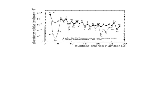
Astrophysical models have to include spallation processes. If one compares
abundances of cosmic rays and solar system elements, it is seen that Li, Be
and B in cosmic rays are enriched by more than 6 orders of magnitude, as
shown in Fig. 1.3.
They were evidently produced in spallation reactions of hydrogen nuclei
(which consist about 87 of cosmic rays) with heavy elements (produced due
to stars explosions). For more informations see [15, 16].
Theoretical predictions of the process are important in each of mentioned above cases. Several models have been constructed in order to describe the spallation process. First stage of the reaction is described by a class of microscopic models, e.g. [17, 18, 19]. For the second stage statistical models are used, e.g. [20, 21]. Nevertheless, the theoretical investigations are rather fragmentary and still not satisfactory. Global qualitative and quantitative informations of the spallation reactions are needed.
Description of global average properties of proton induced spallation reactions in wide range of projectile energy and mass of target nuclei is the main subject of this work. This is investigated within a transport model based on Boltzmann - Uehling - Uhlenbeck (BUU) equation supplemented by a statistical evaporation model. The used transport model has been specially developed in the frame of this work, in order to enable description of such reactions.
This work is organized as follows.
In Chapter 2, present knowledge of the reaction dynamics and review of various
theoretical models is given. Chapter 3 includes description of
the Hadron String Dynamics (HSD) approach of the first stage of the spallation
reaction. In Chapter 4 and Chapter 5, results concerning properties of the first
stage of the reaction are presented and discussed. Chapter 6 concerns pions,
which could be produced only in the first stage of reaction. In Chapter 7,
statistical evaporation models for the second stage are recalled.
Chapter 8 contains bulk model predictions of both stages of
proton - nucleus reactions.
In Chapter 9 and Chapter 10, the models results and comparison with available
experimental data and with results of other models are presented, respectively.
Finally, in Chapter 11, a summary and conclusions are given.
Chapter 2 Present knowledge of the reaction dynamics - basic theoretical models
Our understanding of physical phenomena is expressed as modelling. At present, the broadest platform for such modelling is quantum mechanics approach. Unfortunately, many - body systems are usually an extreme challenge for existing methods of quantum mechanics. One has to rely on rather simple, much more straight formed concepts. In this Chapter, such general basic concepts will be shown as ingredients of typical models of nuclear reaction.
Several microscopic models have been constructed in order to describe the first stage of proton - nucleus reaction. All of them have the same basis, they describe the reaction as a cascade of nucleon - nucleon collisions, but employing different assumptions. The main difference concerns implemented potential of nucleon - nucleus interaction. One can distinguish the simplest models, which neglect features of the mean field dynamics and employ constant static potential, like a class of Intra - Nuclear Cascade (INC) models. Other, more sophisticated approaches comprise dynamically changing field and minimal fluctuations obtained due to use of test particle method, i.e. models based on Boltzmann - Uehling - Uhlenbeck (BUU) transport equation. There are also models, which include real fluctuations and particles correlations, employing two- and three- body potentials, e.g. Quantum Molecular Dynamics models. The main ideas of the different types of nuclear reaction approaches are described below.
In this Chapter, devoted for model-like approach of investigation of nucleon - nucleus reactions, also so-called percolation model is presented. This rather basic model describes fragment mass distributions very well (Section 2.3).
2.1 Intranuclear Cascade model
Intranuclear cascade (INC) model is used as a base in many existing codes for
the first stage calculations.
Description of the nucleon - nucleus reaction in terms of binary nucleon -
nucleon collisions inside nucleus is the basic assumption of the model.
In principle, the single particles approach of the INC is justified as long as
the de Broglie wavelength of the cascade particles is smaller than
the average internucleon distance in the nucleus ( 1.3 fm).
This indicates the low energy limit of the model
(e.g. for projectile kinetic energy MeV
fm, for MeV fm).
The INC calculations follow the history of individual nucleons that becomes
involved in the nucleon - nucleon collisions in a semi - classical
manner. It means, the momenta and coordinates (trajectories) of the particles
are treated classically. The only quantum mechanical concept incorporated in
the model is the Pauli principle.
The first code of INC has been created by Bertini [22], in 1963.
Later, the conception was used also in other codes, e.g. by Yariv in his ISABEL
code [23]. In the 80’s and 90’s, the next versions of INC model was
developed by Cugnon et al. [17].
The main features of the standard INC approach are the following.
The initial positions of target nucleons are chosen randomly in a sphere of
radius fm, where: is the mass number of
target nucleus.
Momenta of the nucleons are generated inside a Fermi sphere of radius
MeV/c.
Neutrons and protons are distinguished according to their isospin.
All nucleons are positioned in a fixed and constant, attractive potential well
of MeV depth, inside the nuclear target volume.
The depth value is taken a bit higher than the Fermi energy
( MeV), so that the target is stable during the reaction.
The idea of fixed average potential is based on a relatively low number of
particles emitted during the INC stage of reaction, which disturbes the mean
field only slightly.
The incident particle (of incident energy ) is provided with an impact
parameter , chosen randomly on a disc of radius . It is positioned at
the surface of nucleus, in the potential . Its kinetic energy is equal
to .
Relativistic kinematics is used for description of the reaction (i.e. the total
energy of a nucleon is connected with its momentum and mass by relation:
).
All nucleons are propagated in time; their momenta and positions
are evolved in time as follows:
,
.
At time , the incident nucleon is hitting the nuclear surface.
Next, all particles are moving along straight line trajectories, until two of
them reach their minimum relative distance, or until one of them hits the
nuclear surface.
When a particle hits the nucleus surface from inside, two cases are considered.
If the kinetic energy of the particle is lower than the , it is
reflected on the surface. If the kinetic energy is higher than the ,
the particle is transmitted randomly with some probability, see Ref.
[17].
A collision takes place, if the minimum relative distance between
two particles fulfills the condition:
, where: is
the energy in the center of mass of the two particles, is the
total collision cross section.
The two particles are scattered elastically or inelastically, according to the
energy - momentum conservation.
Inelastic collisions with high probability lead to the formation of Deltas
(’s). Mass of
is introduced with the Lorentzian distribution centered on the mean
value equal to 1232 MeV, with the width =110 MeV.
The following reactions are considered in the model:
, , , ,
.
All used cross sections and angular distributions are based on available
experimental data [17].
Additional condition restricting a collision is Pauli blocking. Collisions and
- decays are avoided, when the presumed final states are already
occupied. The final states phase - space occupation probability ( and
, where and denote two particles predicted to be created in the
final state) is evaluated by counting
particles of the same kind, inside a reference volume in phase - space. The
collision or decay is realized, when: is larger
than a random number chosen between 0 and 1.
The interaction process is stopped at time , determined by the
average behaviour of some quantities (e.g. an excitation energy of the nucleus,
see Ref. [17]).
At the end of the cascade, all remaining ’s are forced to decay.
2.2 Quantum Molecular Dynamics model
Quantum Molecular Dynamics (QMD) [19, 24] model has been
developed mainly in order to investigate fragments formation during
proton - nucleus or nucleus - nucleus collisions.
The model,
as a N-body theory, describes the time evolution of correlations between
particles,
what is essential in consideration of the fragments formation.
In the approach,
nucleons are spread out in phase - space with a Gaussian distribution.
The coordinates and momenta of nucleons are designated simultaneously.
The wave function of each nucleon () is assumed to have the following
Gaussian form:
| (2.1) |
where: the Gaussian width - - corresponds to a root mean
square radius of the nucleon of 1.8 fm, are the coordinates
of the centers of the Gaussian wave packets.
The normalized Gaussian function represents one nucleon.
In the model, Szilard-Wigner densities are applied. Those give a semi-classical
approximation, depending simultaneously on coordinates and momenta. The
Szilard-Wigner density is defined by the following expression,
constructed of a wave function: [25]:
| (2.2) |
This is called the probability function of the simultaneous values of coordinates: and momenta: . It has the following properties. Integrated with respect to the , it gives probabilities for the different values of the coordinates:
| (2.3) |
Also, integrated with respect to the , it gives quantum mechanical probabilities for the momenta :
| (2.4) |
Based on upper definition, the Szilard-Wigner representation of considered in the model system is given by:
| (2.5) |
The boundary distributions, i.e. the densities in coordinate and momentum space are given by:
| (2.6) |
| (2.7) |
In order to construct the initial system, the centers of the Gaussians (i.e. nucleons) are chosen randomly in coordinate and momentum space, in the following way. First, the positions () of nucleons are determined in a sphere of the radius . The numbers are chosen randomly, rejecting those which would position the centers of two nucleons closer than fm. In the next step, the local density (), at the centers of all nucleons, generated by all the other nucleons is determined. Then, the local Fermi momentum () is calculated: . Finally, the momenta () of all nucleons are chosen randomly, between zero and the local Fermi momentum (). Then, all random numbers, which position two nucleons in phase - space closer than: are rejected, and must be chosen again. The initialization process lasts long time. Typically, only 1 of 50 000 initializations is accepted under the criteria. But the finally accepted configurations are quite stable, usually no nucleon escapes from the nucleus in 300 fm/c, see [19].
After successful initialization, the nuclei (in case of nucleus - nucleus
collisions) are boosted towards each other with the proper center of mass
velocity.
During propagation, only positions () and momenta () of nucleons
() are changed, the width of the wave function is kept fixed.
The mean values are evaluated at time under the influence of
two- and three- body interactions (important for preserving the correlations
and fluctuations among nucleons), according to the classical Newtonian
equation of motion:
| (2.8) |
with the Hamiltonian , where: is total kinetic energy and is
total potential energy of all nucleons.
Usually, the differential equations are solved using an Eulerian integration
routine with a fixed time step , where the momentum is evaluated at
time points halfway between the times of the position determinations:
| (2.9) |
Assumed in the model total interaction is composed of a short range
interactions between nucleons (), a long range Yukawa interaction
(,
fm) and a charge Coulomb interaction (, stands for charges).
Potential acting on each particle is given by the expectation value of the two
and three body interaction:
| (2.10) |
where the two body potential is given by local, Yukawa and Coulomb interaction terms, while the three body potential includes only the local interactions term, see Ref. [19].
Two nucleons can collide if they come closer than ,
where is a total nucleon - nucleon cross section.
Additionally, Pauli principle is taken into account.
In the model, the measured free nucleon - nucleon scattering cross section is
used. However, the effective cross section is smaller because of the Pauli
blocking of the final state. It means, whenever a collision has occurred, the
phase - space around the final states of the scattering partners is checked.
It is calculated, which percentage, and , of the final phase -
space for each of the two scattering partners, respectively, is already
occupied by other nucleons. Then, the collision is blocked with a probability
, or allowed with the probability .
If a collision is blocked, the momenta of scattering partners are kept with
values, which they had before scattering.
The scattering angles of the single nucleon - nucleon collisions are chosen
randomly, with the probability distribution known from the experimental
nucleon - nucleon scattering [26].
Inelastic collisions lead to the formation of Deltas, which can be reabsorbed
by the inverse reactions.
It is assumed in the QMD approach, that only these beam energies are accepted,
at which no more than of all collisions are blocked. Therefore, the low
energy limit of the model is kinetic energy MeV/nucleon
[19].
2.3 Percolation model
Percolation model has been introduced in the eighties as minimum information
approach, based on purely topological and statistical concepts. It was in order
to describe fragment size distributions, as an outcome of nuclear
fragmentation process within the simplest possible physical framework
[27].
However the model is flexible enough to allow for the inclusion of different
physical mechanisms.
In general, one distinguishes between bond and site percolation model.
Site percolation corresponds to the case where each site is either occupied by one particle or is empty. One fixes a probability , and for each site generates a random number , taken from a uniform distribution in the interval . If the site is said to be occupied, if it is empty. Checking all sites, one obtains an ensemble of occupied and empty sites. Sets of occupied sites are called clusters. Finally, space is topologically covered with clusters and empty space.
Bond percolation corresponds to the case where each site is occupied, but neighbouring sites being bound or not to each other. The number of neighbouring sites is fixed by the bonds, which depend on the geometric structure of space occupation. A similar procedure, as in case of site percolation, works also in this case. For a fixed bond probability one considers a pair of neighbouring sites and generates a random number . If the sites are linked by a bond, if they are not. Checking all possible bonds between neighbouring sites one obtains clusters made of connected particles. There are clusters of different sizes, appearing with a given multiplicity, which depends on .
The first applications of percolation concepts were proposed by W. Bauer and
collaborators [28, 29], Campi and Desbois [30].
While Campi and Desbois used a site percolation, Bauer with his group have
proposed a model based on bond percolation theory. Nowadays, the bond percolation has been used as a base for models of fragmentation more often than the site one. Below, an outline of model proposed by Bauer et al. is presented.
As any percolation model, it is based on two crucial ingredients: a description of the distribution of a set of points (i.e. nucleons) in a space and a criterion for deciding whether two given points are connected.
The target nucleons are represented by points occupying uniformly an approximately spherical volume on a simple cubic three-dimensional lattice in coordinate space.
The lattice spacing is computed from the normal nuclear density:
, where: .
The number of points is equal to the number of target nucleons and is conserved during the calculation, therefore the conservation law of mass in the calculated fragmentation process is fulfilled.
Initially, each nucleon is connected by bonds (representing the short-ranged nuclear interactions) to its maximum six nearest neighbors, depending on its location in the target.
Then, a point-like proton, with an interaction radius collides the target.
Because it is assumed that the motion of the nucleons in the target is
neglected, the projectile sees a frozen image of the target (it is feasible, as
typical Fermi motion speed of nucleon is significantly lower than speed of
incoming proton). For a given impact parameter , the proton removes from the lattice nucleons occupying a cylindrical channel with the radius along his straight path in the target. It is typically 6-8 nucleons.
All of remained nucleons, called spectators, are still connected via bonds.
These bonds are then broken with a probability , which is a percolation parameter. The parameter should be related to some physical input.
For example, it is reasonable to assume that is a linear function of kinetic energy of the projectile, and also an increasing function of the excitation energy () of the spectators: , where: is the nuclear matter binding energy per nucleon (16 MeV) [31].
The breaking probability has to be also dependent on the impact parameter of the proton. Bauer et al. have used following dependence: , where: , is a radius of the target nucleus, is a diffuseness parameter [29, 31].
For given parameter , the breaking probability is assumed to be uniform for all bonds, independent of their position on the lattice.
Using the breaking probability as an input parameter, a Monte-Carlo algorithm decides for each bond individually whether it is broken or not, as follows.
For a given , a random number is generated for each bond , where: the indices correspond to the spatial location of the center of the bond on the lattice. If , the bond is unbroken, if , the bond is broken.
Then a cluster search algorithm [29] is used to find out which
nucleons are still connected by bonds i.e. form clusters.
Taking into account all impact parameters, inclusive mass and multiplicity distributions can be obtained. That can be compared to experimental results.
It is surprising that using only one free parameter and simple geometrical
considerations, this model is able to reproduce experimental mass yield curves
with a good accuracy, in particular, the power law behavior
() at small masses and the U-shape distribution of the
whole mass range.
Bauer’s group have used such model also to study the possibility of observing a phase transition of nuclear matter in collisions of high energy protons ( GeV) with heavy targets. Since inclusive fragment mass distributions follow a power law behavior: , for , ( is independent of target mass for heavy targets) [32] similar to the mass yield distribution of droplets condensing at the critical point in a van der Waals gas ( , with the critical exponent ), they suggested that nuclear multifragmentation proceeds via a liquid-gas phase transition of nuclear matter.
Bauer et al. have accented the importance of their result for experimental study of the phase transition, that the critical events are not the ones with the highest multiplicities, but the ones with the highest value of standard deviation of mass distribution.
In the percolation models, such as described above, it is assumed that nucleons are distributed uniformly in the sphere, and the total excitation energy is assumed to be uniformly distributed over the whole excited system of the spectators, what is equivalent to assumption that equilibrium is reached. In this picture, the angular distribution of fragments should be forward peaked, because the momentum transfer from incident proton to the nucleus is in average in forward direction. In reality, as the incident energy increases, the mass fragments angular distribution grows from forward to sideward ( GeV) [33] or backward ( GeV) [34] peaked in laboratory frame, what contradicts to the picture of the fragmentation from an equilibrated system, and indicates that the nucleons may not be uniformly distributed spatially and the excitation may depend on the position inside the nucleus.
For the understanding of this sideward emission (for which not satisfactory explanation has been given so far) Hirata et al. [35] investigated the non-equilibrium dynamical effects, such as non-spherical nuclear formation. They formulated Non-Equilibrium Percolation (NEP) model, which they use in a combined framework with a transport model [35]. The main differences between equilibrium percolation and the NEP model are following. The initial conditions of percolation, instead of putting nucleons on sites with some assumed occupation probability, is taken from the results of the dynamical transport model calculations. The bond breaking probability is assumed to be dependent on the position and momenta of the nucleons. It is calculated by considering excitation energy, distance and momentum difference between the nucleon pairs, instead of giving a common breaking probability for the bonds connecting nearest neighbor sites.
Analysing fragmentation process with the NEP model, considering calculated
effects, Hirata et al. have found following mechanism of sideward enhanced
fragments emission. Based on fragments formation point distributions, both in
case of central and peripheral collisions, the fragments are formed mainly near
the surface of the nuclei. It is due to fact, that along the incident proton path, nucleons collide with the leading proton or secondary cascade particles. Since they have large kinetic energies, they increase the bond breaking probability. As a result the fragment formation is suppressed along the incident proton path. Fragments are formed mainly in the cold region around the hot zone. Their formation points are distributed non-spherically, in a doughnut shaped region. Hirata et al. noticed that this effect alone does not generate any anisotropy in angular distributions.
Based on analysis of fragments energy distributions, they found that the energy
distribution is effected by Coulomb repulsion.
Calculated results after the Coulomb expansion well reproduce the qualitative behavior of experimental data [35].
This is Coulomb repulsion between formed fragments that pushes and accelerates them sideways of the doughnut region. It means, the Coulomb repulsion modifyies the angular distribution from forward peaked to sideward peaked.
Bond percolation model with non-equilibrium effects, have been investigated also by Yamaguchi and Ohnishi [36].
They introduced to the model isospin dependence, by assuming that neutron-neutron and proton-proton bonds are always broken, while neutron-proton bonds make the nucleus bound. Additionally, by comparing calculated fragments energy spectra with experimental data, they have got an agreement, when taken density of fragmenting nuclei is not equal the normal nuclear density , but of around . It means, target nucleus, after being heated by incident proton, would expand up to rather low, mechanically unstable density.
They have also considered, that the incident proton heats up either cylindrical or conic shaped region around its path in the target. They have found, that in
case of cylindrical heated region, formed fragments are pushed, by Coulomb
repulsion, more strongly in sideward directions. If a conic shaped region is
heated up, fragments are pushed in rather backward directions.
Chapter 3 Specific models for fast stage of proton-nucleus collision
In the frame of this work, dynamical analysis of fast stage of proton - nucleus
reactions are performed within transport approaches:
Boltzmann-Uehling-Uhlenbeck (BUU) [18, 37] and Hadron
String Dynamics (HSD) [38, 39] models. The models have been
specially developed in order to enable description of considered here
reactions.
The BUU model is used to calculate proton - nucleus reactions in
projectile kinetic energy range only up to about 2.5 GeV.
That is because included in the
model processes go mainly through single resonances excitations (i.e. ,
(1440), (1535)), what is correct in this energy range. While an incident
energy increases, the density of produced resonances also increases. In this
case, a possible proper description of processes requires taking into
consideration hadron - hadron reactions on the level of elementary quark -
quark interactions. This can be done by employment of a string model
(e.g. FRITIOF model [40]), where during inelastic collision, two
interacting hadrons are excited due to longitudinal energy-momentum transfer
[40].
The formed excitation, so-called string, represents a prehadronic stage. It is
characterized by the incoming quarks and a tubelike colour force field
[41] spanned in between. The string is then allowed to decay into
final state hadrons, with conservation of the four-momentum, according to e.g.
Lund string fragmentation model [42].
The HSD approach includes the FRITIOF scheme of string dynamics and the Lund
model of hadron production through string fragmentation. It is employed, in
particular, for incident energies higher than projectile energy 2.5 GeV. For
projectile energies lower than about 2.5 GeV, the BUU code is used in the
frame of the HSD model.
Below, a description of the approaches is given.
Both the models are based on transport equation.
3.1 Transport equation
Historically, the transport equation originate from classical Boltzmann
equation for one-body phase-space distribution function
defined such that
is the
number of particles at time positioned in element volume around
, which have velocities in volume element of velocity space
around .
Let’s consider particles, in which an external force with mass acts and
assume initially that no collisions take place between the particles.
In time the velocity of each particle will change to
and its position will change
to . Thus the number of particles
is equal to the number of
particles ,
what is explained by the Liouville theorem:
The volume of phase-space element is constant, if movement of all particles inside is consistent with canonical Hamilton equation of motion.
and written as:
| (3.1) |
If collisions occur between the particles, an additional element, i.e. collision term is needed. This gives the following equation describing evolution of the distribution function:
| (3.2) |
Letting and expanding into the Taylor series gives the Boltzmann equation:
| (3.3) |
An apparent form of the collision term can be
found considering an element volume A at time , around position
() and an element volume B at time , around
position ().
These two element volumes are so similar, that letting ,
particles knocked out from A, due to collisions, will not get into
B. Particles being outside A, during time , will get into
A, and they will be inside B. So, the number of particles inside
B, at time , at , is equal to the
initial number of particles inside A, at time , and a magnitude of
relative modification of number of particles due to collisions, during time
.
Therefore, a form of the collision term can be
calculated as a difference between the number of collision in a time range
(), when one of particles after collision is situated in
element volume around position (), and
the number of collision in a time range (), when one of particles
before collision is situated in the same element volume around position ().
It can be done by assuming that the density of particles is low enough, that
only binary collisions need be considered. It is also assumed that the velocity
of particle is uncorrelated with its position in the space. It means that in
element volume the number of particles pairs with velocities in volume
elements of velocity space around and
around is equal to:
.
The number of binary collisions (,
, ) inside element , in time range
is equal to: ,
where:
and are the velocities of the two particles before
collision,
and are their velocities after the collision,
is the differential cross section for a reaction, in the
centre of mass reference frame,
is the solid angle the particles are scattered into (the angle between
vectors i ),
is the magnitude of the particles relative
velocity before the collision,
is
the density of particles flux equal to the product of particles density and
their velocity.
The total number of collisions, where one of the particle before
collision is situated inside element around
() is obtained multiplying the number of binary
collisions by number of particles with velocity , inside element
and integrating over all possible and :
| (3.4) |
Taking into consideration the inverse binary collision: (, , ), and using analogical method as above, the total number of collisions, where one of the particle after collision is situated inside element around () is obtain:
| (3.5) |
Because collisions , ,
and , ,
are inverse collisions, so: .
From covservarion law for energy and momentum: .
From Liouville theorem: .
Subtracting equations (3.5) and (3.4), and
using above assumptions the collision term can be written as:
| (3.6) |
where:
, ,
, .
Joining equations (3.3) and (3.6) one obtains the classical Boltzmann equation:
| (3.7) |
where:
,
, is position
dependent potential.
In 1933 Uehling and Uhlenbeck have developed the equation by adding the Pauli
factors [43].
Due to Pauli blocking, a collision can occur only if in the final state, there
are free quantum states.
Probability of finding the free quantum state in a
phase-space volume is equal to: , what is
responsible for fermion Pauli blocking.
The probability of two particles
collision with momenta and is equal to:
| (3.8) |
Including in (3.7) the Pauli factors gives:
| (3.10) |
The equation is named Boltzmann-Uehling-Uhlenbeck (BUU) equation.
3.2 Boltzmann-Uehling-Uhlenbeck model
The theory based on the transport equation (3.10) (it means the
Boltzmann equation with a self-consistent potential field, and with a collision
term that respects the Pauli principle) was used first time to nuclear
collisions description by Bertsch, in 1984 [44].
The BUU equation is solved numericaly, using Monte Carlo method, representing
the one-body phase-space distribution by discretized test particles:
| (3.11) |
where:
is a number of test particles,
is a number of real particles at time
Likewise, one collision is replaced by parallel collisions.
All of the test particles give part to the density of nuclear matter not in
single points, but they are smeared with Gauss distribution. This way, the
effect of quantum smearing is included.
The density is calculated on the grid :
| (3.12) |
where: is the Gauss width parameter (taken usually equal 1).
The initial coordinates of particles of target nucleus have Wood-Saxon distribution form:
| (3.13) |
where:
= 0.5
.
Initially, the target nucleus is in the rest, the total momentum (i.e. the sum of momenta of all particles) is equal to 0, but the local momenta of particles are determined homogeneously on the Fermi sphere with radius :
| (3.14) |
The projectile is a single proton. The test particles replacing the proton are distributed homogeneously on a thin cylinder, with a radius equal the radius of target. Thanks to this approach, each test particle has different impact parameter, so the results of calculations are averaged over all impact parameters.
The solution of the transport equation is the single-particle phase-space
distribution function, depending on time.
The collision is numericaly evolved by fixed time steps.
The test particles propagate between collisions according to the classical
Hamilton equations of motion:
| (3.15) |
| (3.16) |
where: is a mean field potential, dynamically changing, calculated as a function of local density:
| (3.17) |
where: =-1124 MeVfm3, =2037 MeVfm4,
=-378 MeV, =2.175 fm-1, see Ref. [18].
The momentum and coordinates of all particles taking part in reaction are
calculated in the successive time steps.
Using the values of momentum and coordinates, all other quantities (i.e.
nucleon density, mean field potential) are calculated.
The nucleon - nucleon collision at a fixed time step is introduced as follows:
when two nucleons come closer than the distance (where is the maximal cross section for
nucleon - nucleon interaction in nuclear matter (30 mb [18])) they
are made to scatter, but if the final state is Pauli blocked, this collision is
canceled.
The BUU model describes the propagation and mutual interaction of nucleons,
Delta’s, - resonances, and also and - mesons.
In the model, the following reaction channels are included:
,
,
,
,
,
(1535) ,
,
,
,
where: is a nucleon,
stands for a resonance , (1440) or (1535).
Cross sections for the reactions, used in the model calculations, are
parametrizations of the experimental cross sections taken from [45].
All resonances are allowed to decay into two particles (besides the decays due
to collisions with other particles, e.g. ).
The decay of a resonance is determined by its width . The decay
probability is calculated in every step of time, according to the
exponential decay law: ,
where: is the energy dependent width of the resonance,
is a Lorentz factor related to the velocity of the resonance,
is a time step size of the calculations.
For the decay the parametrization given by Koch et al. [46]
is used. Details concerning higher resonances can be found in [47].
In each step of time it is decided if the resonance may decay and to which
final state it may go. If the final state is Pauli blocked, the resonance decay
is rejected.
3.3 Hadron String Dynamics model
The HSD model is based on the same transport equation (3.10) as the
BUU approach and solved also by use of the test particle method.
In the HSD model, propagation of the following real particles are included:
baryons (, , , (1440), (1535), , ,
, , ), the corresponding antibaryons and mesons
(, , , , , , , , ).
3.3.1 Cross sections
The low-energy baryon-baryon and meson-baryon collisions (i.e. with the invariant energies below ”string threshold”: GeV and GeV [39], respectively) are described using the explicit cross section, as in the BUU code. The following parametrization of the experimental total and elastic , , , , , cross sections, taken from [45], is used:
| (3.18) |
where: is a momentum of incident proton in laboratory frame,
, , , , are constants, with adequate values for different
processes cross sections, see Ref. [48].
For reaction channels: and
, to have them consistent with the experimental inelastic
pion-proton cross section below the string threshold, instead of
(3.18), the following parametrization is used [48]:
| (3.19) |
where: is a momentum of incident pion (in GeV/c).
Additionally, the channels:
, and
, ,
are included with an energy independent cross section equals to 30 mb.
Because of very low number of produced hyperons in low-energy proton-nucleus
collisions, the hyperon(, ) - nucleon interactions are
neglected in the model.
Angular distribution of elastic collisions depends on energy [48], therefore the following parametrization of the differential elastic nucleon - nucleon cross section, taken from Cugnon et al. [26], is applied:
| (3.20) |
where:
is the invariant energy of collision squared (in GeV),
is the four-momentum transfer squared,
.
In the approach, the high-energy elastic and total baryon -
baryon and meson - baryon collisions (i.e. with energies above the
”string threshold”), are related to the measured cross sections by:
,
,
,
,
where dots stand for other combination in the incoming channel, with
and . The same relations are applied
for the total cross sections.
The high-energy inelastic baryon - baryon and meson - baryon
cross sections obtained by this procedure are equal to 30 mb and 20 mb,
respectively. This corresponds to the typical geometrical cross section
(i.e. ), so it should be reasonable input for
the calculations.
Due to this fact, in order to include all baryon - baryon and meson - baryon
high-energy inelastic cross sections, only final state rates must be specified.
Therefore, the string model (i.e. FRITIOF model) is employed, which will be
described hereafter in this work.
In the HSD model, the following meson - meson reaction channels are
included:
,
,
,
,
.
They are more probable at high-energy proton - nucleus collisions, but as
they appear as secondary or higher order reactions, the average energy for such
processes is rather low. In this case, the cross section within the
Breit-Wigner parametrization is employed. Therefore, the reactions
, where: , , , are the
mesons in the initial and final state, respectively, and denotes the
intermediate mesonic resonance (, , , ), are
described by:
| (3.21) |
where:
and are spins of the particles,
is spin of resonance;
and are partial decay
widths in the initial and final channels,
is the mass of the resonance,
is the total resonance width,
is the initial momentum in the resonance rest frame.
The decay widths and the branching ratios for the mesonic channels are adopted
from the nuclear data tables [45], without introducing new parameters.
Additionally, strangeness production in meson - meson collisions is
included, with an isospin averaged cross section [49]:
| (3.22) |
where: , stands for all possible non-strange mesons
in the incoming channel (e.g. ,
).
3.3.2 String Model
Quarks, as colour-charged particles cannot be found individually. They are
confined in two- or three-quarks systems, i.e. colour neutral hadrons.
The quarks, in a given hadron, exchange gluons. If one of the quarks is pulled
away from the other quarks in the hadron, the colour force field, which
consists of gluons holding the quarks together, stretches between this quark
and its neighbers.
Because of interaction between gluons [41], the colour field lines
are not spread out over all space, as the electromagnetic field lines do, but
they are constrained to a thin tube-like region. While the quarks are pulled
apart, more and more energy is added to the colour force field. So, in such a
formation, the four-momentum can be accumulated. At some point, it is
energetically possible for the field to break into new quarks.
The four-momentum is conserved, because the energy of the colour force field is
converted into the mass of the new quarks. Finally, the colour force field
comes back to an unstretched state.
With this picture in mind, high-energy hadron - hadron interactions models,
called string models [39] have been created, where the formation
composed of quarks and the colour field between is called a string.
In the HSD approach, in order to describe the high-energy inelastic
hadron - hadron collisions, FRITIOF model is applied [40].
In the model, hadronic collision corresponds to large longitudinal and small
transversal energy - momentum transfer. It means, to the stretching of
longitudinally extended string-like colour force field along the beam
direction, between constituent quarks of the incoming hadron. The created
excitation, i.e. string is a dynamical object, which may decay into final state
hadrons, according to the Lund fragmentation scheme [42],
implemented in the FRITIOF model.
The field between quarks is confined into a tube, called ”flux tube”, which is
one-dimensional object. The uniform colour field contains constant amount of
energy stored per unit length. The total energy () of the field is
proportional to the length (): , where
GeV/fm, is a string tension [42]. Due to longitudinal energy-momentum
transfer, spread over some region, the colour separation occurs, i.e. as seen
in CM string frame, there will be two extended parts of the string moving
forward and backward, along the beam direction. The potential between quarks is
linearly rising.
As result, the system breaks. Because of colour confinement there is never a
single quark in isolation. After the string breaks, on its ends new quarks
appear. The new pair is created from the available field
energy. By that means, the energy of the initial string decrease (a part of the
energy is used for pair production), but the breaking process
is not finished yet. The quarks of the new created strings are also moving in
opposite directions in the strings rest frames. Thereby the original system
breaks into smaller and smaller pieces, until only physical hadrons remain,
(i.e. baryons as bound systems of three quarks, antibaryons - three antiquarks
and mesons as quark - antiquark systems).
In the HSD approach, baryonic () and mesonic ()
strings are considered.
The implementation of the string model into the transport approach implies
introduction of a time scale for the particle production processes. The time
scale is given by a formation time , which includes formation of a
string, fragmentation of the string into small substrings due to
and production, and formation
of physical hadrons.
The formation time should be also related to the spatial extension of the
interacting hadrons. It means, it should be big enough so that quark -
antiquark pair could reach a distance corresponding to a typical hadron radius,
i.e. 0.6 - 0.8 fm [48].
In the HSD model, the formation time is a single fixed parameter for all
hadrons, it is set to fm/c in the rest frame of the new produced
particles [50].
The particles production proceeds as follows.
If a system contains originally e.g. and , moving in
opposite directions with large energies, it breaks after some time into two
parts by a production of a pair , at a space-time
point (, ). The new produced quarks also move in opposite
directions. Two subsystems are created by and
. As a result, a colour force field between the new
pair vanishes. At a later time another pair
can be produced at (, ), due to
breaking e.g. subsystem. Analogically, new
subsystems and are
created. A colour force field between the new quark pair
vanishes. Created subsystems either are hadrons or else
will fragment further, until only hadrons remain. In the model, string
fragmentation starts always in its center (in the CM frame of the string).
All quark pairs production points are separated in a space-time.
A total momentum in the rest frame of a string is equal to zero.
The energy and momentum in the production process is conserved.
Masses of the finally produced hadrons are equal to the masses of physical
hadrons.
In the HSD model, the production probability () of massive
or pairs is supressed in
comparison to light quarks pairs production (,
). Inserting the following constituent quark masses:
GeV and GeV, one gets:
and
.
So, the suppression factors used in the model are:
: : : = 1 : 1 : 0.3 : 0.07, see Ref. [48].
As a result, mainly mesons are produced.
The model assumes that there is no final state interaction of the produced
hadrons included in the model.
Because most of the strings, in a given space-time volume, fragment within a
small time interval, the interaction of the string field spanned between the
constituent quarks with other hadrons is not taken into account. But the
secondary interactions of the quarks or diquarks inside the strings are
considered in the approach. The following cross sections of such interactions
are used [48]:
mb,
mb,
mb.
Because most of strings are stretched longitudinally, parallelly to each other,
and radius of string is small, equal to about 0.2 - 0.3 fm [51],
there is no string - string interaction included in the HSD model.
The characterized above version of the HSD code has been used and developed
in order to describe proton induced spallation reactions in wide energy range,
and mass of target nuclei in the following aspects. First of all, to calculate
properties of residual nuclei remaining after first stage of the reaction,
forming an input for models of the second stage calculations.
Additionally, the code has been developed for description
of pions produced in proton - nucleus spallation reactions.
Moreover, a version of HSD code that allows for calculations of pion induced
reactions has been prepared.
Each of the directions of the HSD code development will be presented and
discussed in the next sections of this work.
3.4 Further development of the model
As a result of the first stage of proton - nucleus reaction, apart from
emitted particles (mainly nucleons and pions), a hot excited nucleus remained.
Properties of the residual nucleus, i.e. mass (), charge (),
excitation energy (), three - momentum () and angular
momentum () form an input for the second stage models.
In order to calculate the properties, the original version of the HSD code has
been modified.
Corrections ensuring energy and charge conservations have been made,
which are important here, but played minor role in the original version. Also,
corrections enabling calculations of various quantities in function of time,
for very large times of propagation have been found.
The properties are evaluated in the following way.
First, using that in the models calculations, four-momenta of all hadrons
are propagated in time, the particles that have left the residual heavy
fragment are identified. This can be done in two ways.
In case of low-energy collisions, a sphere of observation, with radius equal
to fm, where: denotes the radius of the target with mass
number , can be considered. All the particles inside the sphere are
treated as belonging to residual nucleus, the particles outside - as emitted.
In case of high-energy collisions, when target nucleus is moving faster
during reaction, it is easier to consider a baryon density criterion. It
means, particles, which are positioned in baryon density lower than 0.02
nucleon/fm3
are treated as emitted, the rest of the particles form a residual
nucleus. At intermediate proton impact energy (0.1 - 2.0 GeV) both methods are
equivalent. In the frame of this work, the second criterion is used.
Nevertheless, both of the methods of classification are
connected with some inaccuracy, concerning the very low energetical particles.
Distributions of particles escaped from
the sphere of observation characterize absence of very low energetical part.
In contrary, distributions of particles classified on the base of the baryon
density criterion characterize overabundance in the very low energetical part.
In this second case, it is because the density condition classifies incorrectly
nucleons placed in the lowest density level of a residual nucleus, as emitted.
Therefore, the density method needs to be completed by an additional condition
concerning the particles kinetic energy.
Particles in the nucleon density equal to 0.02 nucleon/fm3
acquire momentum with a value from the range from zero to the local Fermi
momentum, equal to about 130 MeV/c, what corresponds to about 10 MeV of kinetic
energy. Compliance of that information gives a complete and correct condition,
i.e. particles in nuclear density lower than 0.02 nucleon/fm3 and with
kinetic energy higher than 10 MeV are considered as emitted.
Then, by exploring the conservation of total energy, mass number, momentum
and angular momentum, for each parallel ensemble (see description of models),
the average values of properties of the residual nuclei are calculated as
function of time, according to formulas:
| (3.23) |
where: denotes the number of emitted particles, is the mass of the residual nucleus, is a mass of original target, stands for incoming proton and is the the energy of Coulomb interaction between the emitted particles and the residual nucleus.
3.5 Stopping time criteria for the first stage model calculations
In order to describe both stages of the reaction, model of the first stage must
be used together with a statistical model for the second stage of reaction.
The outcome of the transport model calculations determines an input for
the second stage model. Thus, it is important
to assume a proper duration time of the first stage calculations.
In order to define the time at which the first stage calculations should be
stopped, it must be verified, whether informations obtained from the
transport models are sensitive to the time duration of the first stage of the
reaction. For this purpose, time variation of the average values of four
physical quantities: excitation energy per nucleon, momentum in beam direction
per nucleon, angular momentum and mass
number of the excited residual nucleus after the first stage, have been
analysed. As example, the dependences for p + Bi collision, at 3.0 GeV
proton beam energy are discussed below.
The average values of presented quantities
are evaluated according to the equations (3.23).
First, let’s look at the time evolution of the average value of excitation
energy per nucleon of the residual nucleus shown in Fig. 3.1.
It is evident from the Figure, that it takes some time before proton
approaches nucleus, i.e. about 10 fm/c (at the time zero, projectile is
placed in some distance from the target nucleus, ensuring that density
distributions of projectile and target are not overlapping).
Next, up to about 18 fm/c, the
excitation energy gains some maximal value, which corresponds to the energy
introduced into target nucleus by incoming proton. Then, the excitation energy
drops very quickly in the range 20 - 30 fm/c of the duration time of the first
stage of the reaction, whereas it is varying only a little at larger times. It
is seen that the average value of excitation energy per nucleon starts to
stabilize at time 35 - 40 fm/c.

Looking at Fig. 3.2, it is seen, that the average value of the momentum of the nucleus in the beam direction behaves very similar during first stage of the reaction as the average value of excitation energy.

Starting from about 10 fm/c, when proton reaches target nucleus, up to about 18
fm/c, the longitudinal momentum per nucleon of the residual nucleus has a
maximal value, adequate to the value of momentum introduced into target nucleus
by incoming proton. Then, the average value drops quickly in the range 20 - 30
fm/c of the duration time of the first stage of the reaction, because the
momentum is carried out by nucleons escaping from the nucleus. At larger times
the value varies only a little.
Very similar behavior is observed for the average value of angular momentum of
the residual nucleus during first stage of the reaction, presented in Fig.
3.3.

At about 10 fm/c, incoming proton, having in
average a non zero impact parameter, introduces some angular momentum into
the nucleus. At around 18 fm/c and later the angular momentum lowers
significantly due to nucleons escaping from the nucleus. This leakage of
angular momentum stops at around 30 fm/c and the average value stabilizes.
At later time, i.e. from about 40 fm/c, spurious slow increase of angular
momentum is observed, which is unphysical and results from building-up
inaccuracies of numerical calculations. That also indicates that
the first stage calculations should be terminated at about 35 fm/c.
Looking at the time evolution of the average mass number of the residual
nucleus, presented in Fig. 3.4, quite different behavior is
observed.

It is seen, that at about 10 fm/c the projectile come into the target nucleus.
As expected, the mass number is increased by one. But then, starting from
about 18 fm/c, the mass number of the residual nucleus decreases monotonically
with duration time of the first stage of reaction and does not stabilize at
larger times, as it was in case of the other quantities.
This indicates, that emission of particles in this model takes place all the
time. Duration time of the cascade of the nucleon - nucleon collisions
cannot be determined on the basis of behavior of the average mass number of
the nucleus. Nevertheless, it accents the importance of assumption of a proper
stopping time for the calculations, which has influence on a value of
multiplicity of emitted particles. It has a negligible meaning for
energy distributions of ejectiles, since, as a time evolution of excitation
energy shows, from about 18 fm/c, particles with lower and lower energies are
emitted.
The behavior of excitation energy, longitudinal momentum and angular
momentum as a function of time shows that choice of the stopping time is
limited from two sides. The first stage calculations cannot be terminated too
early, when interacting system is highly nonequilibrated.
From the other side, also not too late, since for longer
times numerical inaccuracies are increasing.
Based on above dependences, it is concluded that the most reasonable duration
time of transport models calculations of the first stage of proton induced
reactions is equal to 35 fm/c.
Behavior of the time dependences in case of reactions on other targets nuclei and other values of incident energy is displayed in Fig. 3.5.
It is seen that stabilization of the average values in time depends both on
incident energy and mass of target. The heavier target is used, the
later stabilization occurs. Similarly, the lower projectile energy, the longer
time of first stage calculations is needed in order to reach equilibrium.
Unfortunately, it cannot be assumed one maximal time for all systems, because
of building up of the numerical inaccuracies (see the time dependences of
angular momentum), what starts at different time for different systems.
Nevertheless, the deduced above stopping time equal to 35 fm/c will be treated
in the frame of this work as an optimal time for each system.
It is optimal for all used targets, since it has been
established on the example of one of the heaviest targets. But taking into
consideration dependence on incident energy, the following exceptions must be
included. Calculations of first stage of reactions at projectile energies
greater than or equal to 3.0 GeV, on all targets will be terminated after
35 fm/c. At energies lower than 3.0 GeV, the HSD calculations will be stopped
later, especially for heavier targets.
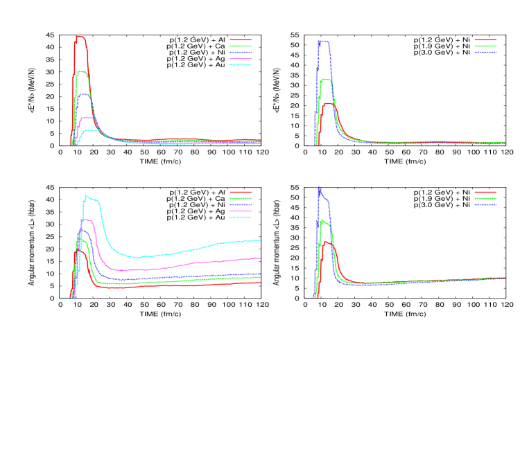
The above considerations are based on the results of calculations averaged over all impact parameters. For particular reaction p+Au at Tp=2.5 GeV, for specific impact parameters, e.g. b = 1 fm, 4 fm, 6 fm, the following dependences: time evolution of average excitation energy (presented in Fig. 3.6), angular momentum (Fig. 3.7) and momentum in beam direction (Fig. 3.8) are obtained.


The example dependences calculated for specific impact parameters agree with results obtained with averaging over all impact parameters; choice of time of calculations of first stage of the reaction ( 35 - 45 fm/c) is satisfactory.
Chapter 4 Bulk properties of the first stage of proton induced reactions
The following scenario of the first stage of proton - nucleus reactions takes place. High energy proton ( MeV) hits a target nucleus. The intra-nuclear cascade starts to develop: the incoming proton, on its way, collides with several target nucleons, transfers energy and momentum to them and may excite them into higher baryonic states. Depending on the position of the cascade nucleons inside the target, they either escape directly from the nucleus or collide secondarily with a few other nucleons transfering further the energy and momentum. Some of the nucleons may leave the nucleus. Development of the cascade can be seen by observing variations of spatial nucleon density with the reaction time. It indicates that proton induced reactions are low-invasive processes.
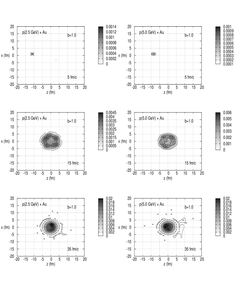
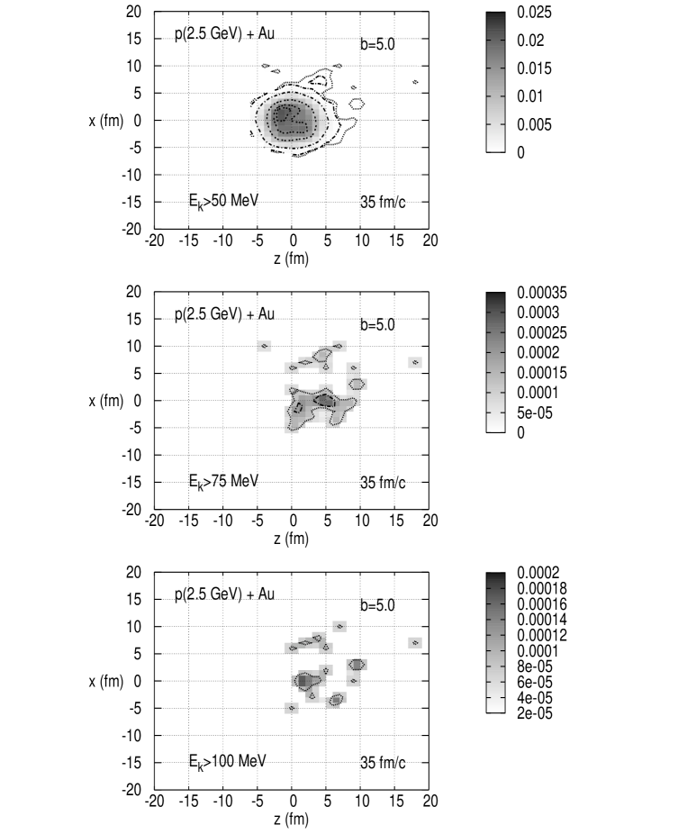
In Figure 4.1 the HSD simulations of time
evolution of nucleon density in central collisions of 2.5 GeV and 5.0 GeV
proton with Au nucleus are presented. The density of nucleons with kinetic
energies MeV has been calculated, in order to see
more clearly the development of the intra - nuclear cascade.
Initially, before proton strikes the target nucleus, the maximal
kinetic energy of nucleons in the target is equal to the Fermi energy ( MeV). As a consequence of interaction nucleons get more energetical.
At the beginning of reaction, the incident proton is in distance of 15 fm
from the center of target nucleus. Projectile enters the target from
the left, is the axis in beam direction.
One can see in the Fig. 4.1, that after 5 fm/c
(1fm/c s),
when proton has not entered the target yet, none of target nucleons has kinetic
energy more than 50 MeV.
Then, looking at the situation corresponding to density distribution sampled
after 15 fm/c, one observes something like a wave going near the surface of
target nucleus. Mainly nucleons from the most outer area of nucleus take part
in the cascade. The center of target is not touched yet.
Situation after 35 fm/c, it means after first fast stage of the reaction
is shown on the bottom plots of the Fig. 4.1.
It is seen that the center of the nucleon density distribution is now
occupied by the cascade nucleons. But the density is not spatially uniform.
The central area corresponds to the maximum of the distribution.
Levels of constant nucleon density (in units nucleon/fm3),
with values increasing to the center of the circular shaped distribution are
clearly visible. It means that in the residual nuclei, the density distribution
of shape like of initial target nucleus is reproduced (the density of initial
nucleus have the Wood-Saxon distribution form (3.13)).
Nevertheless, a small expansion of the nucleus is observed.
The level corresponding to the spatial density of value less than about 0.002
nucleon/fm3 is associated with the free nucleons knocked out of the
target.
Distribution of the nucleon density of residual nuclei, in general, does not
depend significantly on the centrality of proton - nucleus collision. This is
illustrated in Fig. 4.2, where
two-dimensional projections of the nucleon density of residual nuclei, for
different centralities of 5.0 GeV proton with Au nucleus collision are compared
(i.e. for impact parameters of b=1.0, 2.5 and 5.0 fm).
However, on the level corresponding to the lowest spatial density, associated
with emitted nucleons, some differences are observed. They indicate that
more nucleons are emitted in central than in peripheral collisions.

All the presented distributions of nucleon density show that in general, the incoming proton has caused only minor changes of density inside target nucleus.

One of characteristics of created target nucleus is its maximal density. Modification of the density due to penetration of the nucleus by incoming proton is the characteristic feature of proton induced reactions. Such modifications are presented qualitatively in Fig. 4.3, as time evolution of a ratio of maximal nuclear density in case of p+Au reaction at 0.5 GeV, 1.0 GeV, 2.5 GeV and 5.0 GeV of incident energy and the standard nuclear density . It is evident from the Figure, that the incoming proton causes negligible modifications of nuclear density. Though, it is seen, that in case of low energy projectile the maximal density is first slightly increased and then it decreases. In case of higher energetical proton, first slight decrease and then an increase is observed. That could be explained by a fact that incoming low energy projectile almost stops inside target nucleus, causing increase of density, while higher energy projectile goes faster through the nucleus, pushing nucleons away. Then, the situation is changed respectively, due to acting of mean field potential. Nevertheless, the deviations of the presented ratios from the unity are of order of few percent, what proves that proton induced reactions are quite non-invasive processes.
In order to check, how the kinetic energy is distributed inside the residual nuclei, the following test has been made. Based on p+Au reaction, at 2.5 GeV proton beam energy, nucleons, which take part in the intra-nuclear cascade have been observed. It means, nucleons which gained a significant part of the energy of the projectile (i.e. of MeV, MeV). Most of the observed cases indicated homogeneous distribution of kinetic energy inside the residual nuclei. Partial heating up of the nuclei has been noticed in only about of the cases, in peripheral collisions. Illustration of the exceptional situation is shown in Fig. 4.4, where, starting from the top, the nucleon density of residual nuclei of nucleons with kinetic energies MeV, MeV and MeV, respectively are plotted.
Looking at the plot in the bottom of Fig.
4.4 one can distinguish two differently
excited parts. One part of nucleus is composed of nucleons with kinetic
energies greater than 100 MeV, the second part - of nucleons with kinetic
energies lower than 100 MeV. The highly excited group of nucleons, it is about
10 nucleons with an average total momentum equal to about 560(+/-80) MeV/c.
The less excited part, it is till about 184 nucleons with an average total
momentum equal to only about 190(+/-60) MeV/c.
Similar situation is observed, if looking at a bit lower energetical nucleons,
the central plot of Fig. 4.4, nucleons
with kinetic energies greater or lower than 75 MeV.
In this case, the highly excited
part consists of about 20 nucleons with an average total momentum equal to
about 470(+/-90) MeV/c, and less excited part composed of 174 nucleons with an
average total momentum equal to about 190(+/-60) MeV/c.
One can conclude, that the HSD simulations predict something
like formation of two excited sources of evidently unequal masses.
The smaller source consists of relatively few nucleons (up to 20) and is
rather fast, c. The larger source is built of 170 -
180 nucleons and has velocity c. Similar observation has
been drawn from phenomenological analysis of experimental data presented in
[7].
Chapter 5 Properties of residual nuclei after the first stage of proton - nucleus reactions
As it is mentioned above in this work, as result of the first stage of proton
- nucleus reaction, beside emitted particles, an excited nucleus
remains. It differs from the initial target, in average, by only a few
nucleons in mass number. Properties of the residual nucleus (i.e. mass
(), charge (), excitation energy (), three - momentum
() and angular momentum ()) are evaluated, in the frame of
the HSD model, by exploring conservation laws, according to formulas
3.23.
Results of calculations for reactions on various target nuclei, at different
values of incident energy in range from 0.1 GeV to about 10 GeV,
are discussed below.
Let’s look first at one - dimensional distributions of the quantities evolving
with projectile energy and mass of target.
Histogrammed properties for exemplary reactions of 1.9 GeV proton on light
(27Al), heavy (197Au) and two intermediate mass (58Ni and
107Ag) targets are displayed in Fig. 5.1.
Distributions for proton induced reaction on example Al target, at several
values of proton beam energy are shown in Fig. 5.2.
The average values and standard deviations for the presented distributions are
collected in Tables 5.1 and 5.2.
The Figures 5.1 and 5.2 and values collected in the Tables 5.1 and 5.2 indicate, that all of the distributions differ significantly with mass of target, but behave similarly for varied projectile energies.
| reaction | p+Al | p+Ni | p+Ag | p+Au |
|---|---|---|---|---|
| 23.962.25 | 54.712.65 | 102.243.55 | 192.393.69 | |
| 3.0362.25 | 3.292.65 | 4.763.55 | 4.613.69 | |
| 11.641.42 | 26.531.64 | 45.051.98 | 77.341.92 | |
| 1.361.42 | 1.471.64 | 1.961.98 | 1.661.92 | |
| MeV | 74.5681.77 | 122.84120.41 | 144.16125.65 | 222.16171.24 |
| MeV/N | 3.273.63 | 2.302.29 | 1.431.27 | 1.160.91 |
| 4.773.25 | 7.413.59 | 11.765.50 | 17.148.08 | |
| GeV/c | 0.180.24 | 0.220.27 | 0.290.35 | 0.340.38 |
| GeV/c | -0.00110.28 | -0.00140.31 | -0.00580.36 | -0.00450.37 |
| impact energy | 1.0 GeV | 2.0 GeV | 3.0 GeV | 4.0 GeV |
|---|---|---|---|---|
| 23.512.17 | 24.0322.20 | 24.231.99 | 24.122.085 | |
| 11.281.35 | 11.661.37 | 11.781.31 | 11.711.33 | |
| MeV | 65.7654.067 | 73.4684.27 | 70.3188.081 | 74.5098.023 |
| MeV/N | 2.942.61 | 3.223.75 | 3.0263.84 | 3.254.35 |
| 4.752.65 | 4.713.072 | 4.854.48 | 4.995.23 | |
| GeV/c | 0.180.24 | 0.170.23 | 0.160.24 | 0.160.25 |
| GeV/c | -0.00210.27 | -0.000880.27 | -0.00300.27 | 0.00330.27 |
| impact energy | 5.0 GeV | 6.0 GeV | 7.0 GeV | 8.0 GeV |
| 24.0272.19 | 23.942.26 | 23.862.35 | 23.752.41 | |
| 11.661.39 | 11.6031.41 | 11.581.46 | 11.541.47 | |
| MeV | 74.6190.60 | 76.4898.98 | 79.64129.89 | 81.92137.73 |
| MeV/N | 3.294.13 | 3.414.55 | 3.585.8 | 3.716.29 |
| 5.0345.66 | 5.488.25 | 5.157.32 | 6.03511.044 | |
| GeV/c | 0.160.24 | 0.160.25 | 0.170.27 | 0.180.28 |
| GeV/c | -0.0000240.27 | 0.00530.28 | 0.00260.28 | -0.00510.29 |
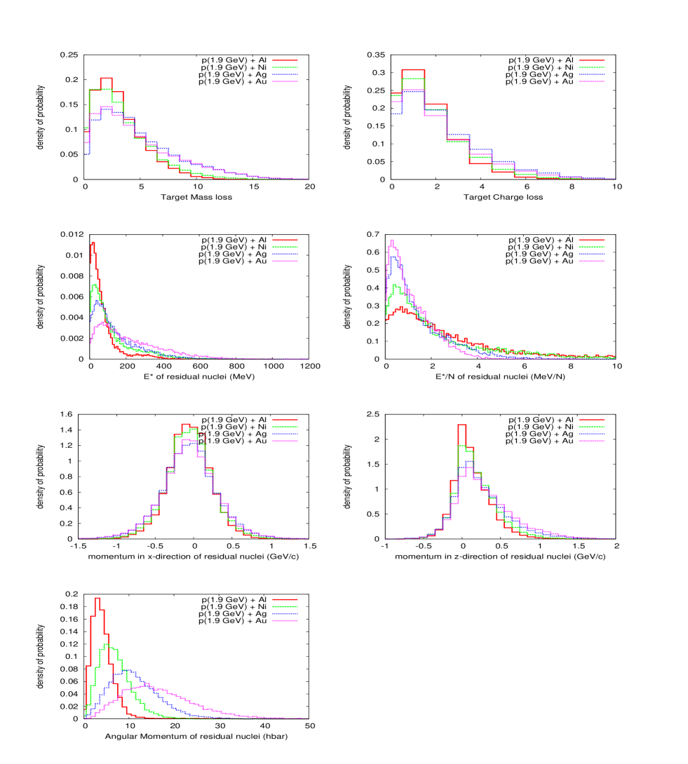
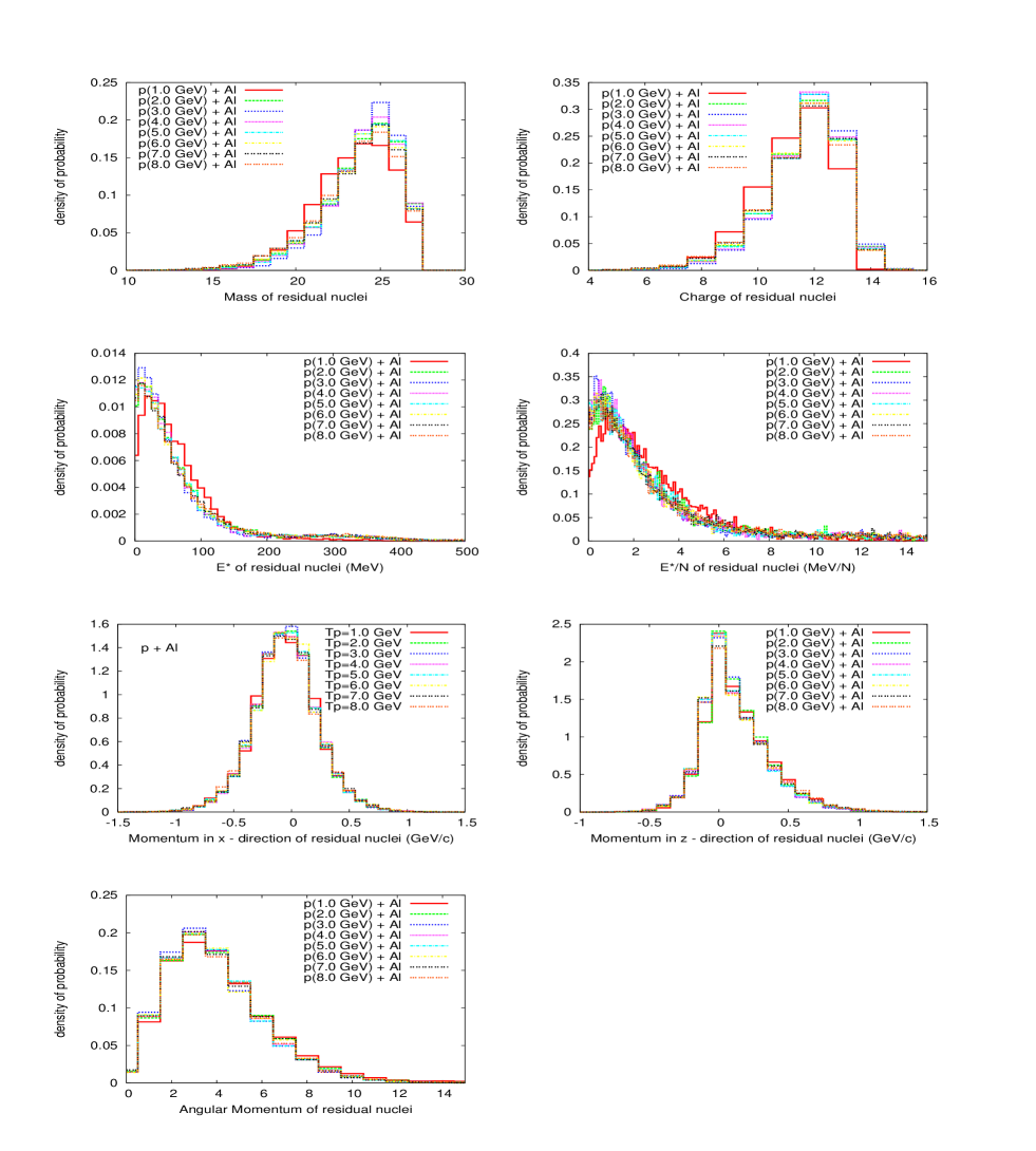
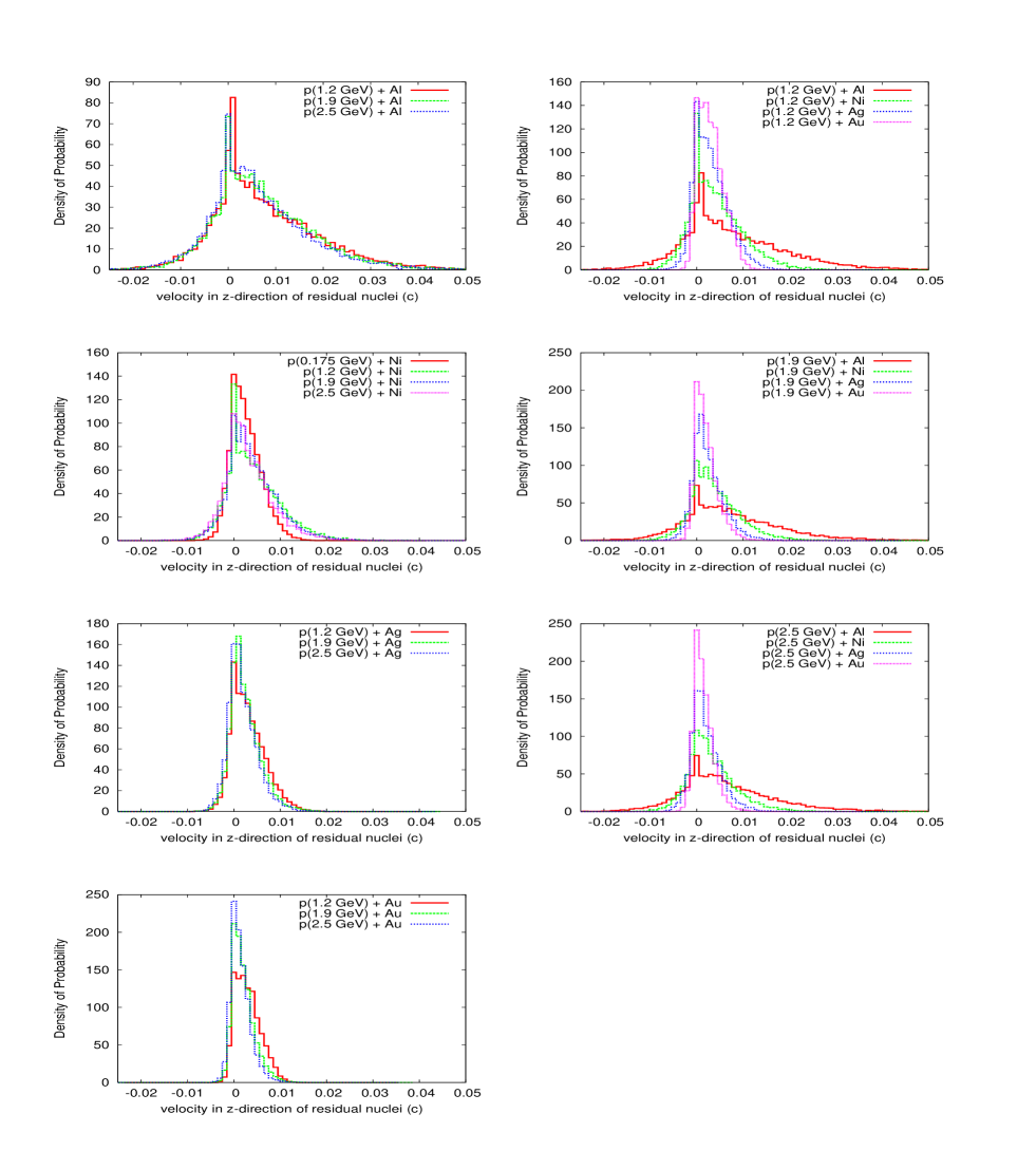
Reason for these behaviors is connected with finite size of nuclei. Average values of excitation energy () and angular momentum () of residual nucleus and width of the distributions increase with mass of target nuclei, at fixed projectile energy. For a chosen target, the distributions of very slightly depend on incident energy. Distributions of almost do not depend on incident energy. This can be explained in an intuitive way by analyzing how the energy and momentum are deposited into a target nucleus. The left in the residual nucleus after the first stage of reaction is in average only a small fraction of the energy, which has been introduced into a target nucleus by incoming proton. Most of the energy is carried away by emitted particles (example energy balance is presented in Sec. 8.1). The number of ejected particles should be treated as a signature how many nucleons were involved in the intra - nuclear cascade. The more nucleon - nucleon collisions inside target nuclei, the larger part of the energy and angular momentum introduced by a projectile is deposited into the residual nucleus. E.g. due to a collision of the incident proton with a nucleon inside a target, a resonance, mainly Delta resonance could be excited. The Delta resonance has a short time of life, i.e. about 1 - 2 fm/c. It decays into nucleon and meson (mainly pion) or collides with other nucleon before the decay. As result, energy is accumulated inside target nucleus. The heavier target, the more collisions can occur, because the cascade of collisions can last for a longer time. For light targets, the excitation energy () is respectively small, because a number of collisions made by a projectile is low. In case of the excitation energy per nucleon () the situation is opposite, i.e. is a decreasing function of mass of target. This is just because in heavier targets, the amount of energy is distributed among more nucleons.
Similarly, distribution of angular momentum of residual nuclei almost does not depend on value of incident energy, but strongly depends on mass of target. The heavier target, the more angular momentum is deposited inside. This is because in the HSD model, quasi - classical approximation for calculations of angular momentum is used; at fixed impact energy, the maximal angular momentum of projectile is proportional to radius of target nuclei. Therefore, in case of heavier targets, more angular momentum is introduced by a projectile.
Distributions of momentum in beam direction (z-component) and the momentum perpendicular to the beam direction (x-component) indicate that residual nuclei are moving according to initial direction of projectile. It is evidently seen (both from the Fig. 5.1 and Table 5.1), that the average values of momentum in x-direction of residual nuclei are consistent with zero.
| c | p+Al | p+Ni | p+Ag | p+Au |
|---|---|---|---|---|
| =1.2 GeV | 0.00820.011 | 0.00460.0056 | 0.00360.0036 | 0.00350.0027 |
| =1.9 GeV | 0.00780.011 | 0.00440.0054 | 0.00290.0033 | 0.00250.0024 |
| =2.5 GeV | 0.00690.010 | 0.00360.0052 | 0.00240.0032 | 0.00190.0021 |
Similar information about the reaction could be extracted from distributions of velocity in beam direction of residual nuclei. The distributions differ significantly with mass of target, but behave similarly for varied projectile energies, as shown in Fig. 5.3. The average values and standard deviations of the values are presented in Table 5.3. It is seen that the lighter target, the broader is the distribution. These are asymmetric, peaked in forward direction, with tails in backward direction. This indicates, that in average, the residual nuclei tend to move forward, according to the initial direction of projectile.
In order to have a better view of the dependences, average values of the quantities and standard deviation of the average values, have been expressed as a function of incident energy and mass of target and presented in Figures 5.4 and 5.5.


Average values and standard deviations of mass number and charge of residual nuclei remaining after first stage of p+Al reaction, in function of projectile energy are presented in Figures 5.6 and 5.7. It is interesting, that both the mass number and the charge, in average, increase up to 3.0 GeV of incident energy. Then decreasing is observed. The ratio of average values of the mass number and charge is constant as function of projectile energy, as shown in Fig. 5.8. Additionally, it exceeded the ratio for initial target nucleus.


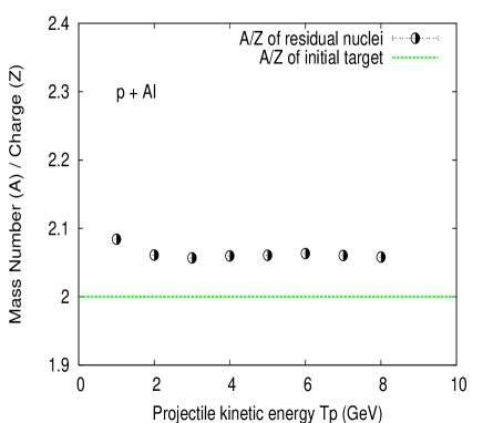
Average values and standard deviations of momentum in beam direction of residual nuclei after first stage of proton induced reaction on several targets, at various incident energies are presented in Fig. 5.9.


One can conclude, that the heavier the target, the more momentum in beam
direction is deposited inside. What more, the maximum in mass dependence on
projectile kinetic energy (at the incident energy equal to 3.0 GeV) for given
target, see Fig. 5.6, corresponds to the minimum of dependence of
momentum in beam direction of residual nuclei in function of projectile
energy.
Behavior of standard deviations as function of projectile kinetic
energy is noteworthy. It is observed, that the higher incident energy, the
broader are distributions of excitation energy, momentum, angular
momentum, mass number, charge of residual nuclei.
This can be qualitatively explained taking into account results of simulations
presented in the Fig. 5.10 (i.e. dependence of multiplicity
and energy of emitted nucleons during the first stage of the reactions on
incident energy).
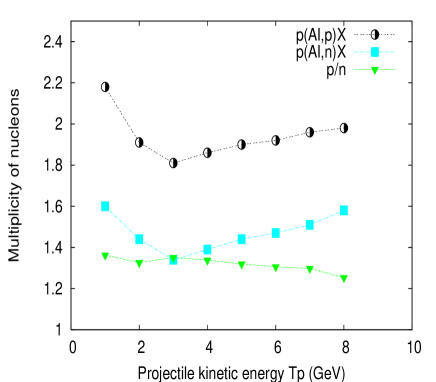
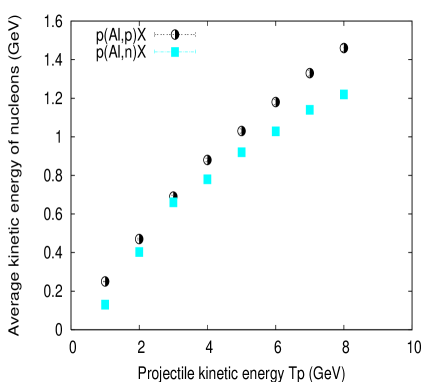
The behavior of multiplicity of emitted nucleons as function of projectile energy perfectly agrees with the behavior of mass and charge of residual nuclei. It means, first, up to about 3.0 GeV of incident energy, number of emitted nucleons decreases, so that mass of residuum increases. With further increase of impact energy, more and more nucleons are emitted, so that mass of the residuum decreases. Obviously, average kinetic energy carried by emitted nucleons is a monotonically increasing function of projectile energy in the whole considered range of projectile energy, as shown in Fig. 5.10. Protons carried out in average more kinetic energy than neutrons, since more protons than neutrons are emitted during first stage of reaction. The p/n ratio is larger than unity, because of the extra proton correspondig to the incident particle (see Fig. 5.10). One can conclude that information of type of projectile is somehow remembered by the system during the first stage of reaction (this topic is undertaken also in Sec. 8.2).
Looking at behaviors of average values of properties of residual nuclei,
especially their momentum in beam direction, mass number and multiplicity of
emitted nucleons during first stage of reaction as function
of incident energy, it is seen that the average values first continuously
decrease (or increase, respectively) with the incident energy, up to about 3
GeV and then consistently, the opposite tendency is observed. The precise
explanation of such behavior is difficult, it must be a result of a few
simultaneous effects. Newertheless, considering elementary processes
(implemented to the model, based on experimental data), one can suggest the
following qualitative explanation.
Such behaviors should be connected with contribution of different
resonances excitations, which depends on the energy introduced by a projectile
into the target nucleus.
At low projectile energy (about 1.0 GeV) nucleons are emitted mainly due to
elastic nucleon - nucleon scattering. More probable than at higher energies is
also, that incoming proton stops inside target nuclei.
At higher incident energies possibility of excitation of resonances (mainly,
the most important here resonance) increases.
A bit less, but more energetic nucleons are emitted. In result, the average
multiplicity of emitted nucleons decreases,
so mass of residual nuclei increases and the average longitudinal momentum
decreases.
At higher incident energy (equal to about 3.0 GeV), from one side the
probability of resonance excitation becomes smaller, and from the
other side probability of excitation of higher resonance is still too low.
This corresponds to the minimum (or maximum) of the incident energy dependences
of the considering quantities. Then, with further increase of projectile
energy, probability of excitation of other resonances increases.
This causes, that more energy and momentum is deposited into residual
nuclei. So, the average longitudinal momentum of residual nuclei increases.
Simultaneously, more particles could be produced, since the ratio of inelastic
to elastic collision increases. The multiplicity of
emitted nucleons increases, so the average mass of remnants decreases.
Behavior of multiplicity and average kinetic energy of emitted nucleons,
as function of target mass number, at an example impact energy is shown in
Fig. 5.11.
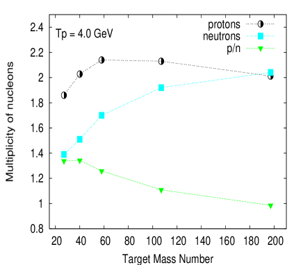
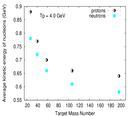
One can see, that the heavier target, the smaller differences in number of emitted protons and neutrons. For the heaviest presented target, the p/n ratio is equal to the unity. One can conclude that in heavy targets, the information about a type of projectile is lost due to possible large number of mutual reactions. Total number of emitted nucleons increases with mass of target nucleus and stabilizes for heavier targets (with mass numbers greater than 60). In heavier targets, the cascade of intra-nuclear collisions can last longer, so that emitted nucleons carries in average less kinetic energy. The nucleon, on its way, going outside the nucleus, has to penetrate through nuclear skin of the nucleus, with high probability undergoes further collisions. As result, more particles with suppressed energies are emitted.
More informations about the excited nuclei is provided by two - dimensional correlation plots of their properties. Example dependences of excitation energy, mass of residual nuclei and their velocity in the beam direction are shown in Fig. 5.12 (velocity versus excitation energy per nucleon and velocity versus residual mass).
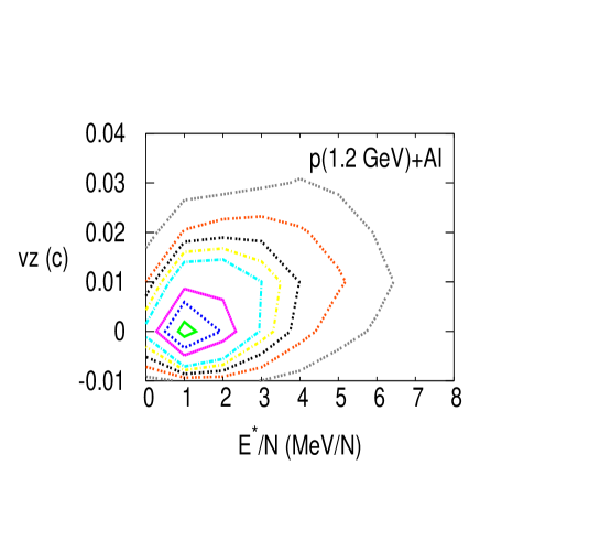
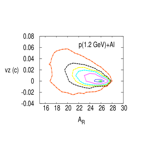
It is meaningful, that velocity in beam direction of residual nuclei increases with increasing excitation energy deposited inside the residual nuclei. This indicates, that the energy is comprised also in onward movement of residual nuclei. Simultaneously, the velocity increases with decreasing mass of residual nuclei, what is equivalent to increase of number of ejected particles. One can conclude that also excitation energy of residual nuclei should increase with decrease of mass of the nuclei. In Figures 5.13 and 5.14, regression function of excitation energy on target mass loss and regression function of angular momentum on target mass loss are presented (for residual nuclei formed in p+Al reaction, at a few impact energies and proton induced reaction on several targets at example 4.0 GeV incident energy, respectively). The dependences are roughly linear functions of the target mass loss.
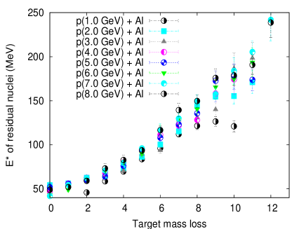

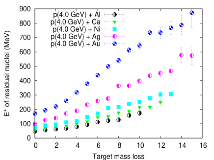
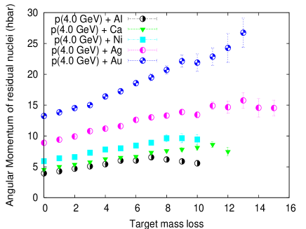
It is seen, that the heavier remnants (for the same initial target), the lower average excitation energy is deposited inside. The average excitation energy increases with decreasing of the remnant mass. Based on the Fig. 5.14, one can conclude that particularly the dependence on mass of target is quite pronounced. It is because, as it is already mentioned above, in heavier targets, where the cascade lasts longer, more energy can be accumulated. In the Figures 5.13 and 5.14, it is also seen, that in the cases of the lowest mass of residual nuclei, (i.e. the target mass loss higher than about 7 nucleons), the increase of excitation energy and angular momentum is not only less pronounced, but even a slight decreases is observed. In such cases, i.e. more ejected particles, the intra - nuclear cascade is lasting for longer time, so that particles with rather moderated energies are emitted.
Example two - dimensional distributions of mass and excitation energy of residual nuclei formed in p+Al reaction, at several projectile energies are displayed in Fig. 5.15. Again, one observes that the higher excitation energy of residual nuclei, the smaller their mass.
Dependence of excitation energy on angular momentum of residual nuclei is presented in Fig. 5.16. The five lines (in upper part of the Fig. 5.16) correspond to the Yrast lines (definition is given in Chapter 7) calculated according to the formula: with different values of the moment of inertia (), where: is the moment of inertia of rigid body (, where and stand for mass and radius of nucleus, respectively), corresponds to the hydrodynamical limit of nucleus (meaning that only a part of nucleus behaves like the rigid body, the other part - in uncorrelated way, see Ref. [52]). One observes that angular momentum increases with increase of the average value of excitaton energy. It is evident, that the dependence is not inconsistent with the Yrast line.

Physicists, who are studing fragmentation have found that this process occurs at some particular value of projectile energy (Tp) (based on (p,7Be) reaction, for various targets at different Tp, see [53]). Fragmentation is a phase transition, what means, that a proper amount of energy needs to be pumped into a system. It follows, that fragmentation occurs at some particular value of , which experimentally has been found to be at least equal to about 5 MeV/N [54, 55].

Using the condition of 5 MeV/N to the HSD model results, presented in Fig. 5.17, it is seen that fragmentation is a very low probable process in proton induced reactions. For example, in p+Al reaction at Tp=5.0 GeV, fragmentation of excited nucleus may occur in about 17 of cases (i.e. the part of spectrum for 5 MeV/N is 17 of the whole spectrum), whereas in p+Au reaction at the same incident energy, only in about 5 of cases. These are cases from the tail of distribution. Based in the Fig. 5.17 one can conclude that fragmentation process is more probable in reactions on light than on heavy targets, and at higher incident energies.
One can suppose that fragmentation of only a part of nucleus could be more probable. This requires inhomogeneous excitation of residual nucleus. It means, not all of nucleons inside the nucleus are involved in carrying of the excitation, i.e. for different target, should be calculated not per each nucleon, but only per some amount of nucleons, which take active part in the cascade. However based on observations of evolution of nucleon density and distribution of kinetic energy inside excited nuclei, it is seen that such partial heating up of nucleus is very low probable. It occurs only in about 1 of cases, as discussed in Chapter 4.
Additionally, experimentalists, who are interested in fragmentation, look for it in central collisions, accompanied with high multiplicity of emitted particles, as it is shown qualitatively by results of the HSD model calculations, presented in Fig. 4.2. Nevertheless, in the HSD simulations, the very low probable partial heating up of nucleus has been found in peripheral collisions (see Fig. 4.4).
Investigated here reactions are very low invasive processes, involving only a few nucleons, causing only minor fluctuations of nucleon density. So, it is evident that there is a negligible probability for fragmentation in proton - nucleus interacting system, in energy range considered in the frame of this work. Spallation is evidently dominant process.
5.1 Parametrization
It is impossible to measure or even to calculate the reaction of proton of
all energies on all target nuclei. One comes to idea to find a global
parametrization for distributions of excitation energy versus mass of residual
nuclei for some chosen sample of targets and energies, involving finally
dependency on the target mass and projectile energy, in order to have the
possibility to interpolate for other energies and targets.
Two-dimensional distributions of excitation energy and mass of residual
nuclei remaining after first stage of proton induced reaction, on a few targets,
at several projectile energies have been parametrized by a sum of at least
three two - dimensional Gaussians:
| (5.1) |
where: stands for heights of the Gaussians, and - define widths in and directions, likewise and - the mean position of the Gaussians in and directions, respectively. Example results of such parametrization are presented in Figures 5.18 and 5.19. It is seen, that the distributions, calculated with the HSD model, are very well described by a sum of Gaussians (5.1).
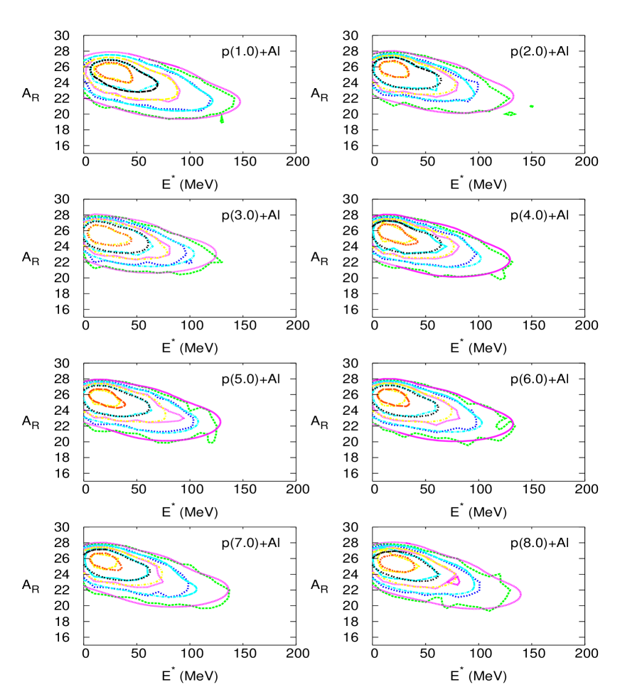
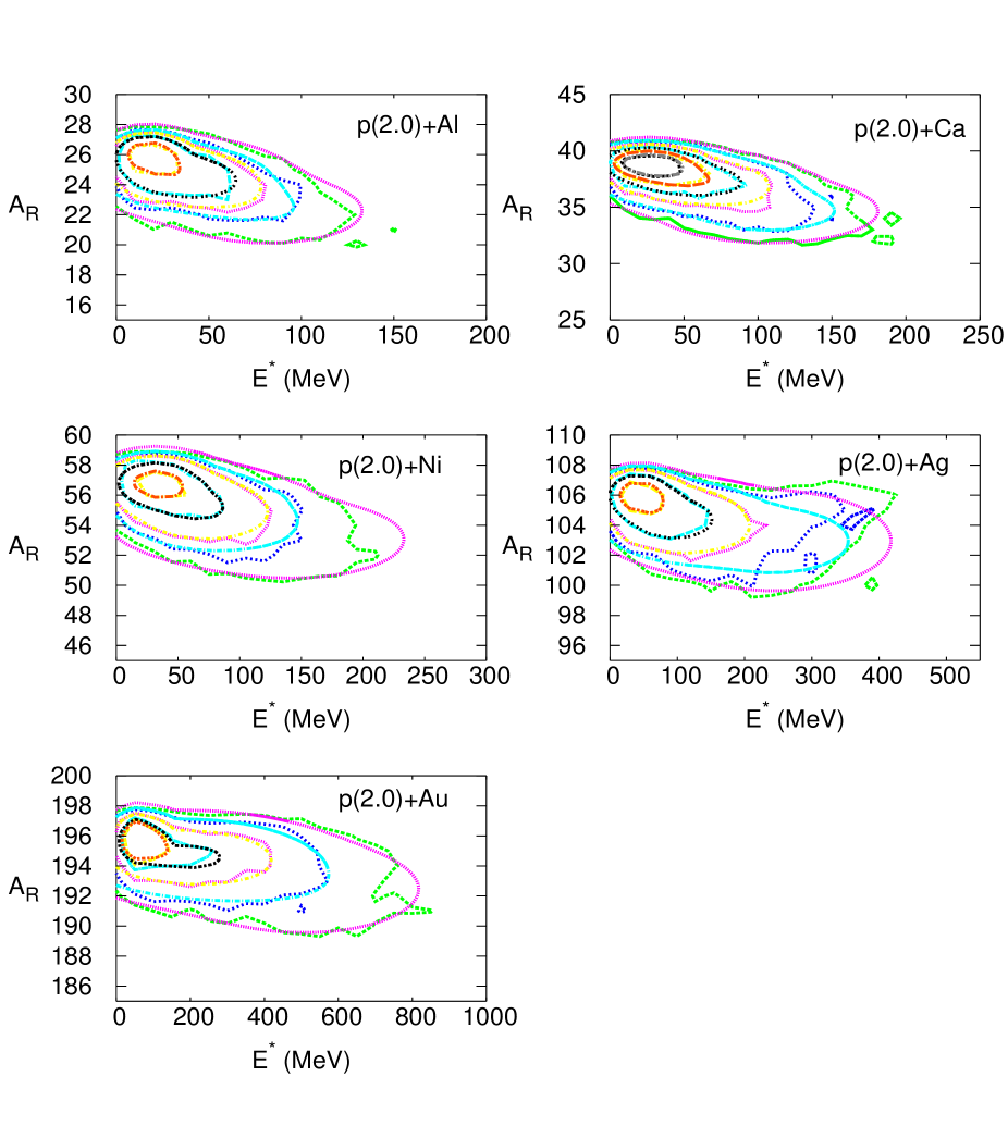
Values of parameters of the Gaussians evolve rather smoothly with incident energy and mass of target nuclei. Example results of parametrization of such dependences are presented in Figures 5.20 and 5.21.
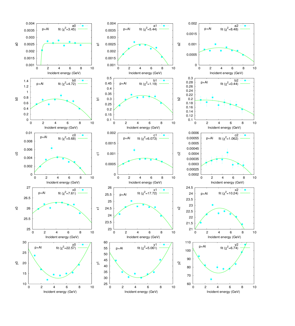
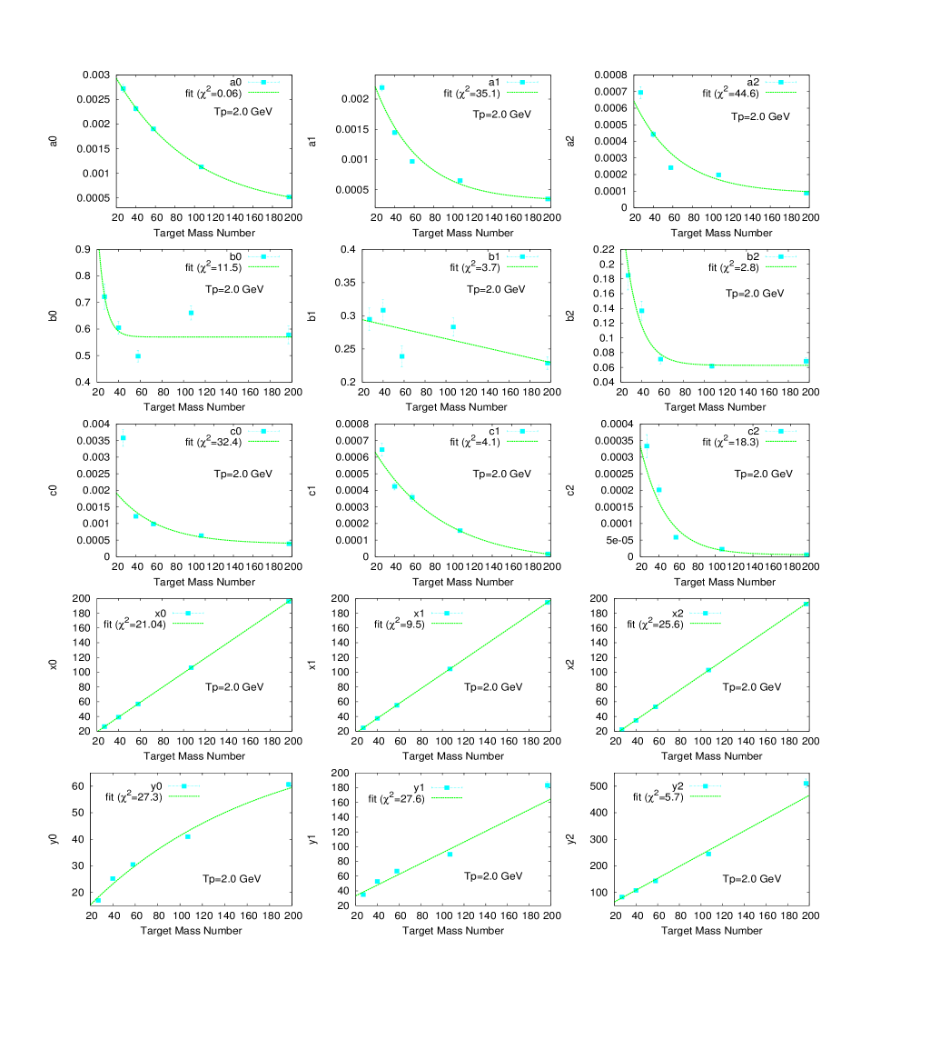
Using the parametrizations, two-dimensional distributions of excitation energy versus mass of residual nuclei could be obtained for any value of projectile energy and target nuclei from the chosen ranges, for the considered cases. In order to verify the parametrization, interpolated distributions have been compared to results of the HSD calculations. Comparisons of distributions for example p+Al reaction at 2.5 GeV beam energy (interpolation of parameters in function of projectile energy, see Fig. 5.20) and p+Zr reaction at 2.0 GeV beam energy (interpolation of parameters in function of mass of target nuclei, see Fig. 5.21) are presented in Fig. 5.22.
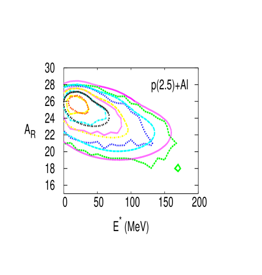
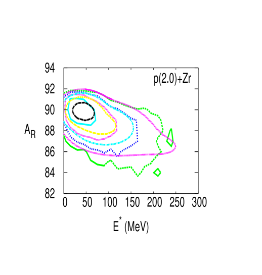
Obtained results are satisfactory. This indicates possibility of realization of such a parametrization for other target nuclei and other incident energies.
Chapter 6 Pion spectra
Pions are the most abundantly produced mesons during proton induced reactions on
atomic nuclei. Creation of pions is very important process in the reactions due
to the fact that they carry away significant part of four-momentum introduced
by incoming particle during the first stage of the reaction.
This is because pion mass ( 140 MeV) is small enough to allow
for copious production of pions in nucleon-nucleon collisions even at low beam
energies, and large enough to contribute significantly to the energy
and momentum transfer.
It should be emphasized that in spite of the fact that momentum
carried away by pions is several times smaller than appropriate
momentum of nucleons (see e.g. the energy balance presented in Sec.
8.1), the contribution of pions to the momentum and
energy transfer may be comparable to that of nucleons. This is because pions,
due to the low production threshold can be produced and reabsorbed
several times during the reaction (threshold for charged pion production in
free nucleon - nucleon collision is equal to about 289 MeV; inside nucleus, it
can be decreased even up to about 141 MeV [56], due to the Fermi
motion). Thus they influence the whole dynamical evolution of the reaction.
Proper treatment of pion production and absorption
may be crucial for realistic estimation of excitation energy and other
properties of residual nuclei after the fast cascade of nucleon - nucleon
collisions.
Calculations of the first stage of the
reaction are sufficient in order to receive realistic pion spectra,
since all pions are produced only in violent nucleon - nucleon collisions,
where the locally available amount of four-momentum is large enough.
One can distinguish two components in pion angular and energy distributions:
high energy anisotropic part, i.e. pions emitted dominantly in forward
direction and isotropic part consisted of low energy thermal pions emitted in
the whole angular range (0∘ - 180∘).
Pions emitted from the first chance NN collisions have high energy, whereas
those from secondary collisions are less energetic.
Building up of pion spectra in time is presented in Figures
6.1 and 6.2.
Typical momentum distributions of pions emitted from 1.0 GeV proton induced
reaction on Al target are shown; corresponds to the momentum
in beam direction. The time evolution of pion distributions is depicted
more precisely in the Fig. 6.2, where
double differential kinetic energy spectra of pions produced during
the example reactions on light (Al) and heavy (Au) target, at low (1.0 GeV) and
higher (2.5 GeV) projectile energy are displayed.
It is seen, that in case of 1.0 GeV proton induced reactions, high energy
anisotropic part of pion distribution is formed first. Then, the isotropic
part is built up. Formation of the low energy part of pion spectra takes longer
time, since it is result of several acts of absorption and emission of pions.
In the Fig. 6.2, all produced pions at the
chosen reaction time are plotted, at further time some of them
can be absorbed or absorbed and re-emitted in other direction, so the number of
presented pions can be lower than at ealier time. After 35 fm/c, all presented
pions are emitted. The number of produced pions is higher in case of 2.5 GeV
proton induced reactions. Pion distributions are evolving with
reaction time only slightly.
At fixed energy of incident protons, pions produced on heavy target are more
abundant than those produced on light target and low energy pions are dominant.
Pion on its way can be several times absorbed and emitted (its mean free path
is equal to 1.0 - 1.5 fm), its initial direction could be changed and its
energy is suppressed. So, it is much more difficult for pion to be emitted
in forward direction in case of heavy target, where it has to pass a longer
distance inside nuclear matter. Therefore, high energy pions emitted in
forward direction dominate in case of light target.
Quantitative comparison of yield of the produced pions is displayed in Table
6.1. It is noteworthy, that almost all of the pions have been
produced due to Delta resonance decay; only a very few pions have been produced
due to N(1440) decay.
| p(1.0 GeV)+Al | p(2.5 GeV)+Al | |||||
| 15 fm/c: | 0.067 | 0.18 | 0.29 | 0.38 | 0.51 | 0.50 |
| 20 fm/c: | 0.071 | 0.18 | 0.29 | 0.37 | 0.47 | 0.47 |
| 35 fm/c: | 0.069 | 0.17 | 0.26 | 0.37 | 0.47 | 0.46 |
| p(1.0 GeV)+Au | p(2.5 GeV)+Au | |||||
| 15 fm/c: | 0.010 | 0.045 | 0.060 | 0.35 | 0.46 | 0.41 |
| 20 fm/c: | 0.085 | 0.19 | 0.26 | 0.53 | 0.60 | 0.52 |
| 35 fm/c: | 0.11 | 0.17 | 0.23 | 0.49 | 0.53 | 0.46 |

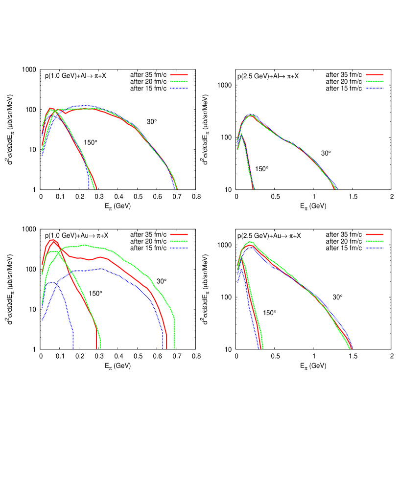

Spectra of pions change significantly with projectile energy.
It is seen in Fig. 6.3, where examplary
distributions of transversal () versus longitudinal () momentum
of neutral pions emitted during proton induced reaction on Ni target
are plotted for various incident energies. These are results of HSD model
calculations, where corresponds to the pion momentum in beam
direction and is defined as .
It can be seen, how the evolution of pion spectra looks like with increase of
incident energy. At low projectile energies pions have not enough energy to
pass through a target nucleus, so they cannot be emitted in forward direction.
In this case, only a small part of target is accessible for pions, the rest of
nucleus corresponds to the so-called nuclear shadow.
Higher pion momenta are associated with increasing incident energy.
With increase of the incident energy, the anisotropic
part of distribution increases. It means, more and more pions have chance to
be emitted in forward directions. The isotropic, low - momentum part of pion
spectra at high projectile energy corresponds to thermal pions, which result
from sequence of several absorptions and emissions.
One should also notice that at high projectile energies (in
the Fig. 6.3 - higher or equal to 2.0 GeV), the isotropic part
of pion momentum spectra is symmetric around .
At low projectile energies
(in the Fig. 6.3 - less than 2.0 GeV), the isotropic part of
spectra, i.e. the most central contour line corresponding to a maximum of
distribution is not symmetric around , but shifted to negative values
of ; to large extent it is due to mentioned nuclear shadow.
The isotropic part of pion spectra that consists of thermal pions has the
Maxwell distribution. This is illustrated by Fig.
6.4, where the experimental distribution of
negative pions, measured by Cochran et al. [57] at backward direction
(150∘), is presented.

The following form of Maxwell function has been used for the parametrization:
where: and are the kinetic energy of the pions
and their mass, respectively. and are fitted parameters.
The following values of the parameters are obtained:
GeV and
GeV.
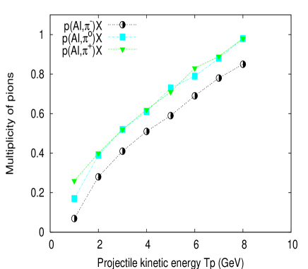
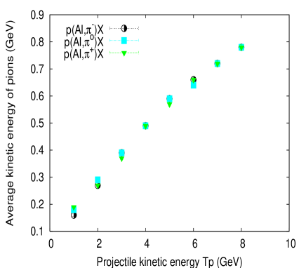
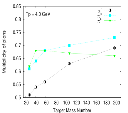
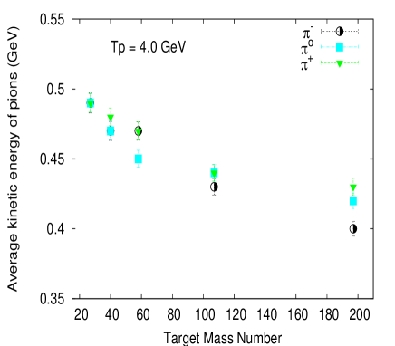
It is interesting to see, how the average yield of pions produced in proton
induced spallation reactions changes with projectile energy and mass of target.
The HSD model calculations predict that multiplicity of pions, in average,
increases both with incident energy and mass of target.
One can expect that due to charge conservation, the relative yield of produced
pions should fulfill the relation: .
The incident energy dependence (presented in Fig. 6.5)
shows, that positive and neutral pion production is favoured, as expected.
For heavier targets, where there are more collisions, multiplicity of positive
pions decreases and for the heaviest target it is even lower than multiplicity
of neutral and negative pions, as displayed in Fig. 6.6.
The target mass dependence shows, that reabsorptions and secondary collisions
play an important role, especially for heavy targets.
Looking at kinetic energy carried by individual emitted pions, it is seen (Fig.
6.5, right) that all kinds of pions produced in
proton induced reactions on a chosen target carry, in average, the same amount
of kinetic energy. The higher energy of the incident proton, the bigger amount
of kinetic energy carried out by pions. In reactions on heavier targets (Fig.
6.6), emitted pions carry away, in average, less
kinetic energy.
In case of the heaviest targets, the negative pions take the least kinetic
energy of all pions. The suppression of kinetic energy of emitted pions from
heavier target is an expected result of numerous possible
reabsorptions and emissions of pions, which become less and less
energetic.
Inclusive differential kinetic energy spectra of pions emitted at different angles, calculated with the HSD model, have been confronted with available experimental data [57], as displayed in Fig. 6.7, for an example distributions of negative pions from p+Pb reaction, at 0.73 GeV of incident energy. One finds, that the calculations overestimate the experimental data.

It is evident, that the pion dynamics in the HSD model needs to be improved, i.e. the number of produced pions should be reduced. Pions are created mainly due to decay of Delta(1232) resonances. It means, pions production and absorption proceeds mainly through the and reactions (see description of the model in Chapter 3). Therefore, modifications of the cross section for the absorption of Delta resonance in reaction and the Delta lifetime should influence the amount of produced pions. In order to estimate the influence, the following corrections have been tested. First, the Delta resonance lifetime has been enlarged. Comparison of the pion spectra calculated with HSD model, with enlarged Delta resonance lifetime and the experimental data [57] is presented in Fig. 6.8 (the calculations are performed with 30 times longer lifetime of Delta resonance). It is seen, that this correction reduces number of pions emitted mainly in backward directions. This is due to the fact, that longer lifetime of Delta resonance implies smaller number of acts of absorption and emission of pions.

If the cross section for the absorption of Delta resonance in reaction is enlarged (by factor 20), the number of pions emitted in forward directions is reduced, as it is shown in Fig. 6.9.

Implementation of both of the corrections reduces the amount of produced pions both in forward and backward directions, as presented in the Fig. 6.10 (these are results of calculations performed with 30 times longer lifetime of Delta resonance and the cross section for its absorption enlarged by a factor 1.5). The improvement of agreement between the data and model results is substantial, however, the introduced modifications are rather drastic. (Improvement of pion dynamics by modifications of Delta resonance lifetime and cross section for Delta absorption has been also performed in frame of the INCL model in [58], but obtained results also do not comply well with experimental data).

Furthermore, it is tested, that the influence of the joined corrections on the pion spectra depends on the value of proton beam energy. The higher beam energy, the lower reduction of the pions yield by the corrections, as it is seen in Figs. 6.11 and 6.12, for spectra of pions produced in p+Au reaction, at low (0.73 GeV) and higher (2.5 GeV) beam energy, respectively. The quantitative distinction of the pions yield from the reactions at two different incident energies are collected in Table 6.2. It has been also verified that implemented corrections do not modify yield and shape of spectra of nucleons. Moreover, the corrections do not influence the properties of residual nuclei after the first stage of reaction. In particular, they do not change excitation energy of the remnants, because the average energy carried out by emitted pions with and without the corrections is the same; due to the corrections less pions are emitted, but they carried, in average, more kinetic energy.
| Tp = 0.73 GeV | Tp = 2.5GeV | |||
| without corrections | with corrections | without corrections | with corrections | |
| : | 0.15 | 0.073 | 0.46 | 0.43 |
| : | 0.11 | 0.053 | 0.54 | 0.48 |
| : | 0.065 | 0.024 | 0.49 | 0.43 |


The not very satisfactory agreement between calculations and experimental data
is not too surprising, because pion production in proton - nucleus collisions
is a complicated process.
Although the elementary cross sections for pions production due to free nucleon
- nucleon interactions are measured and very well known (see e.g.
[59]), in-medium problem appears.
In the HSD model, the in-medium effects are partly included through e.g.
employment of the Pauli principle and cross section for Delta absorption.
However, proper handling of modifications due to in-medium effects are hampered
by a lack of experimental and theoretical knowledge.
Pion production mechanism is highly sensitive to pion
and - resonance dynamics. So, apart from tested above modifications of
the parameters, also introduction of density dependent width of
- resonance (increasing with density), introduction of pion potential,
change of an angular distribution in order to describe possible
anisotropic decay into N channel, etc. can influence the pions
production.
In fact, till now none of the trials have given satisfactory results, see
[60, 61].
The propriety of description of pions dynamics and production due to
proton - nucleus reaction could not be really verified, because experimental
data are rather scarce, especially in projectile energy range of a few GeV
order.
There exists also one more reason that influences the calculated pion spectra. In the HSD model, a target nucleus, i.e. the nuclear density distribution is constructed up to a constant limit , where: is a radius of nucleus, defined as a distance at which the value of nucleus density decreases to a half of the value of density in the center of nucleus; is a mass number of the nucleus; . This is due to difficulties with modelling of the infinite tail of nuclear density at nucleus surface, see [62]. Although the truncated part corresponds to only a small fraction of the whole nucleus density distribution, it can influence the pion spectra. This is because only pions produced close to the surface have a chance to be emitted, as the mean free path of pions is equal to about 1.0 - 1.5 fm, at standard density. The introduced cut off of nuclear surface neglects the possibility of further pion - nucleon interactions at surface, which are quite probable (since pion is a strongly interacting particle) and lead to spuriously higher multiplicity of emitted pions. The nucleus density cut off does not influence nucleons production, because most of nucleons are emitted closer to the center of nucleus, due to the fact that their mean free path is equal to about 3.0 fm. Therefore, the HSD model description of proton induced spallation reaction is not falsified by the used limited distribution of density of target nuclei, only outgoing pion distributions are to some extent misshapen.
Chapter 7 Statistical emission of particles in the second stage of proton - nucleus collisions
The second stage of proton - nucleus reaction can be theoretically described with various statistical models. Historical origin of the models is related to Weisskopf’s paper published in 1937 [4]. Weisskopf considers emission (evaporation) of a neutron with kinetic energy from nucleus , excited to energy , transforming it to nucleus , with excitation energy . Probability of such emission is calculated using the principle of detailed balance. It can be determined if cross section for the inverse process is known (i.e. cross section for production of compound nucleus by collision of a neutron with nucleus ). The probability is expressed as:
| (7.1) |
where: stands for neutron mass, is a spin degeneracy factor,
and are the level densities of the initial and
final nuclei, respectively.
In the Weisskopf expression, angular momentum effects are not taken into
account. In order to consider the effects, one needs to use
the Hauser-Feshbach formalism [63]. In this case, the decay
probability is determined by level density of the residual
nucleus, depending both on its excitation energy and angular momentum
, and transmission coefficient of emitted particle
( is the orbital angular momentum removed by
the particle, is its kinetic energy).
Decay width for state of energy and angular momentum into a
specific channel is expressed as:
| (7.2) |
where: is the level spacing (reciprocal of the level density) of the
decaying nucleus, stands for the particle spin. The following energy and
angular momentum conservation constraints are employed:
,
, where is the binding energy of the emitted
particle in decay channel .
The decay probability into channel is evaluated as:
, where: ,
runs over all open channels.
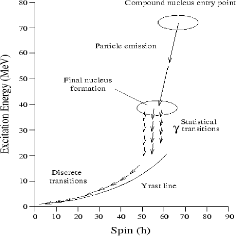
Important step to comprehensive understanding of the dependence of the
level density on angular momentum of compound nucleus was done by J. R. Grover
[64]. He invented the ”Yrast level” term to describe the
lowest lying level at some given angular momentum. It means, that for any
angular momentum the nucleus has to have an excitation energy at least
equals to the rotational energy . Therefore, there cannot be any
states with excitation energy below , i.e. below ”Yrast level”.
Particle decay is inhibited close to the ”Yrast line” (i.e. the level density
is close to zero for the final states allowed by energy and angular momentum
conservation). Deexcitation proceeds mainly by gamma emission along the
”Yrast line”, as illustrated in Fig. 7.1.
In the frame of this work, calculations of the second stage of proton - nucleus reactions have been done with use of PACE2 [20] and GEM [21] codes. Below, basic features and results of the models are presented.
7.1 Evaporation model - PACE 2
The statistical model code PACE2 (Projection Angular-Momentum
Coupled Evaporation, version 2) [20] is based on
the Hauser-Feshbach formalism. The decay sequence of an excited nucleus
is calculated with use of a Monte Carlo procedure, which is followed until the
nucleus reaches its ground state. At each stage of deexcitation, the decay
probability is determined by calculating decay width for neutron, proton,
alpha and gamma. Final states differ in excitation energy, angular momentum,
nucleon number and proton number .
The model contains several parameters, which has to be fixed.
The main ingredients of the code are the level density and transmission
coefficients.
The level density , at a specific value , is given by:
| (7.3) |
where: is the total level density at excitation energy , evaluated according the following formula (given by Weisskopf for Fermi gas, see Ref. [4], [65]):
| (7.4) |
with level density parameter (its dimension is MeV-1).
For selecting the rotational energy contribution, , model of A. J.
Sierk [66] is used.
The transmission coefficients are calculated with use of default
potentials; for protons and neutrons taken from Perey and Perey [67],
for alpha particles from Igo and Huizenga [68].
As the nucleus decays, it is assumed that transmission coefficients of charged
particles are shifted in their kinetic energy dependence: ,
where and are the nucleon and proton numbers of the emitting nucleus,
and is the Coulomb barrier for the emitted particle.
Fission of the excited nuclei is also taken into account.
The fission barrier of Sierk is used [66].
Gamma emission is considered statistically using , , and transition intensities.
7.2 Generalized Evaporation Model
Another model used for the Monte Carlo simulations of the second stage of
the spallation reaction is the Generalized Evaporation Model (GEM),
developed by S. Furihata [21], based on the Weisskopf-Ewing approach
[4, 69].
In the GEM model, 66 nuclides up to Mg are included as ejectiles, not only
the dominant particles emitted from an excited nucleus (i.e. nucleons and
helium isotopes), as it is in the PACE2.
The accurate level density function is used for deriving the decay
width of particle emission, instead of an approximate form, as used in the
PACE2 model (see the previous Section).
Additionally, depending on the excitation energy and mass of the decaying
nucleus, different parametrizations of the level density are
applied, see Ref. [21].
In the GEM model, contrary to the PACE2, the dependence of the level
density on the angular momentum is neglected. Nevertheless, negligible
difference between spectra of evaporated particles, calculated with the PACE2
model, with zero and non-zero values of angular momentum of emitting nuclei,
has been noticed, as displayed in Fig. 7.2.
Adequate multiplicities of evaporated particles, calculated with the PACE2
model, with different values of angular momentum of emitting nucleus are
collected in Table 7.1.

| 0 | 10 | 20 | |
|---|---|---|---|
| n: | 7.80 | 7.80 | 7.70 |
| p: | 0.076 | 0.080 | 0.070 |
| 4He: | 0.031 | 0.031 | 0.031 |
Spectra of evaporated particles (nucleons and 4He) calculated with the PACE2 and GEM models are in good agreement, as shown in Fig. 7.3 for an example Au nucleus, with the excitation energy set to 100 MeV and zero value of angular momentum. Adequate multiplicities of the emitted particles are collected in Table 7.2.

| GEM | PACE2 | |
|---|---|---|
| n: | 8.86 | 7.80 |
| p: | 0.17 | 0.076 |
| 4He: | 0.029 | 0.031 |
Results of the GEM model calculations are very sensitive on the used level density parameter [21]. There is a possibility to use parameter equal to a quotient of mass of emitting nucleus and a constant number MeV-1 (see formula 7.4), where (see Ref.[6, 70]) or one can use the precise Gilbert - Cameron - Cook - Ignatyuk (GCCI) level density parametrization with the energy dependence taken into account, see Ref.[21, 71]. Dependence on the used method of level density parametrization is noticeable e.g. in multiplicities and spectra of evaporated particles. Comparison of spectra of various isotopes evaporated during the second stage of an example p+Au reaction, at 2.5 GeV beam energy, results of the GEM model calculations, with the different level density parameters are presented in Figures 7.4 and 7.5.


It is seen from the Figures, that distributions of light particles
(isotopes of hydrogen and helium) calculated with different level density
parameters are very similar. Contrary, distributions of heavier isotopes
(lithium, beryllium, etc.) differ significantly.
Use of the GCCI level density parameter gives much higher abundance
of the heavier isotopes, than use of the simple parameter.
Moreover, calculations with the parameter result with even higher
abundance than with the GCCI level density parameter.
Adequate multiplicities of the evaporated particles are collected in Table
7.3.
It is seen from the Figures, that choice of level density parameter affects not
only heights of the spectra, but influences also their slopes.
In the frame of the work, the GCCI level density parameter is used
(confrontation with experimental data leads to conclusion, that use of the
GCCI level density parameter gives the most reliable results).
| GCCI | |||
|---|---|---|---|
| n: | 14.78 | 14.90 | 9.016 |
| p: | 1.76 | 1.97 | 0.85 |
| 2H: | 1.11 | 1.11 | 1.17 |
| 3H: | 0.51 | 0.44 | 0.78 |
| 3He: | 0.063 | 0.062 | 0.12 |
| 4He: | 0.84 | 0.76 | 0.85 |
| 6He: | 0.012 | 0.0083 | 0.059 |
| 6Li: | 0.020 | 0.013 | 0.17 |
| 7Li: | 0.018 | 0.012 | 0.22 |
| 8Li: | 0.0055 | 0.0032 | 0.104 |
| 9Li: | 0.0011 | 0.00057 | 0.035 |
| 7Be: | 0.0021 | 0.0016 | 0.027 |
| 9Be: | 0.0039 | 0.0024 | 0.081 |
| 10Be: | 0.0045 | 0.0024 | 0.11 |
| 11Be: | 0.00041 | 0.00019 | 0.021 |
| 8B: | 0.00006 | 0.00004 | 0.0013 |
| 10B: | 0.0022 | 0.0013 | 0.060 |
| 11B: | 0.0018 | 0.00091 | 0.076 |
| 12B: | 0.0011 | 0.00053 | 0.039 |
| 13B: | 0.00013 | 0.00005 | 0.0049 |
| C: | 0.0027 | 0.0015 | 0.093 |
| N: | 0.0011 | 0.00055 | 0.071 |
| O: | 0.00041 | 0.00025 | 0.034 |
Chapter 8 Bulk models predictions for the proton induced nuclear reactions
8.1 Illustration of energy balance of the reaction
In order to show, how large fraction of energy is carried out
during the first and the second stage of proton - nucleus reaction,
respectively, a sample case of the HSD and statistical evaporation model
calculations, for p + Au collision at 2.5 GeV proton beam energy is analysed
in this Section.
The total initial kinetic energy introduced into nucleus by incoming proton is
equal to 2.5 GeV. During the first stage of the reaction, about 1.7 GeV of the
energy is carried away by nucleons and about 0.4 GeV - by pions.
The multiplicity of nucleons is near 4.43, whereas the pion multiplicity,
summed over all pion charges, is equal to 1.48.
The average kinetic energy of one nucleon is about 0.4 GeV, whereas the average
kinetic energy of one pion is equal to 0.29 GeV.
Non-negligible amount of energy is taken away from the excitation energy and
converted into rest masses of emitted pions, i.e. 0.2 GeV.
Remaining energy of the excited nucleus after the first stage
of the reaction, is equal to only about 200 MeV.
This amount of energy is then evaporated in the second stage of the reaction by
emission of mainly neutrons, protons, alphas and gammas.
Emitted neutrons accumulate about 20 MeV of the energy, protons carried
about 3 MeV, alphas - about 1 MeV, and gammas - about 6 MeV.
The multiplicity of neutrons is equal to about 10 and the average kinetic
energy of one neutron is equal to about 2 MeV, multiplicity of protons is equal
to about 1 and the average kinetic energy of one proton is equal to about 3
MeV. Multiplicity of alphas is equal to about 0.3 and the average kinetic
energy of one alpha is equal to about 4 MeV and finally multiplicity of gammas
is equal to about 6 and the average kinetic energy of one gamma is equal to
1 MeV.
After taking into account the binding energy of nucleons inside nucleus, i.e.
about 8 MeV per one nucleon, the whole amount of excitation energy of the
residual nucleus (about 200 MeV) is carried out during the second stage of the
reaction.
The presented balance shows, that the biggest amount of initial energy
deposited in nucleus by incoming proton is carried out during the first stage
of the reaction, i.e. about 85 , and only about 15 of the initial
energy is carried away during the second stage of the reaction.
8.2 Participation of fission processes in spallation reaction
During the second stage of the proton - nucleus spallation reaction, deexcitation of the hot residual nucleus by evaporation of various isotopes takes place, as it is mentioned above in this work. However, there is a possibility, that during this process the evaporating nucleus undergoes fission. In such case, the particles emission is continued from the fission fragments. Probability of fission of particular nuclei depends on the ratio of Coulomb energy and surface energy of individual nucleus. The probability is strongly dependent on fissility parameter () defined as:
| (8.1) |
where: is the charge of a nucleus and is the mass number of a nucleus.
For example, the fissility parameter for Au nucleus, calculated according to the definition (8.1) is equal to 31.7. The experimental data collected in Ref. [72] indicate, that Au nucleus has rather low probability for fission, in comparison of Th and U nuclei. Distribution of the fissility parameter for residual nuclei emerged after the first stage of an example p+Au reaction, at 2.5 GeV beam energy (result of the HSD model calculations) is presented in Fig. 8.1.

The average value of the fissility parameter distribution is equal to .
On the base of a behavior of the fissility parameter in function of mass of residual nuclei, it can be tested if a ratio of charge and mass number is constant during the reaction and equal to the ratio of charge and mass number of the initial target nucleus. The fissility parameter in function of mass of residual nuclei for the example p+Au reaction, at 2.5 GeV proton beam energy is presented in Fig. 8.2.

The ratio of charge and mass number of the Au initial target nucleus is equal to: Z(Au)/A(Au) = 79/197 = 0.40. Using the definition of the fissility parameter (8.1) and assuming that: Z=0.40A, it is obtained that: f=0.16A. Parametrization of the dependence presented in the Fig. 8.2, by a function proportional to the mass number give exactly the same result as received from the definition. This indicates, that in a first approximation, a ratio of charge and mass number is constant during the reaction and equal to the ratio of charge and mass number of the initial target nucleus. However, parametrization of the dependence by a function proportional to some power of the mass number (correcting a slope) gives a bit better accuracy, as presented in Fig. 8.3.

It means, that the ratio of charge and mass number is not exactly equal to the ratio for the initial target nucleus. This is confirmed by multiplicities of protons and neutrons emitted during first stage of the p+Au reaction, at 2.5 GeV proton beam energy. Namely, due to interactions inside the target nucleus, multiplicity of emitted protons (equal to 1.66) is a bit higher than multiplicity of emitted neutrons (equal to 1.63). Contrary, in case of n+Au reaction, at 2.5 GeV neutron beam energy, multiplicity of emitted neutrons during the first stage of the reaction (equal to 1.89) is a bit higher than multiplicity of emitted protons (equal to 1.38). This indicates, that information about type of projectile is kept during the first stage of reaction.
If looking at the kinetic energy distributions of isotopes emitted during the second stage of p+Au reaction, calculated with blocked and allowed fission, differences are visible, because Au nucleus possesses non-zero, although rather small fissility. The example spectra (result of the GEM model calculations) are presented in Fig. 8.4.

It is clearly seen from the Figure, that fission shifts spectra of emitted particles down in their maximum and causes them wider in energetical range, in direction of both lower and higher energies (in Fig. 8.4 the effect is shown for alpha particles). This is because of evaporation from fission fragments, which move in opposite directions. As a consequence there is a bit less particles with intermediate energies, emitted from the unfissioned residuum, but more particles with a bit lower and higher energies, emitted after fission, from excited fragments moving in backward and forward directions, respectively.
Cross section for the different fragments production in function of the fragments masses and charges (result of the HSD+GEM model calculations), for the example p+Au reaction, at 2.5 GeV proton beam energy, calculated with blocked and allowed fission, are presented in Fig. 8.5. Interesting result is obtained, when one subtracts the cross sections obtained with blocked and allowed fission.

One can see in the Figures that fission diminishes amount of nuclei of masses close to 150 - 160 and increases amount of nuclei of masses in the range 60 - 100. One can conclude, that fission is much slower process than evaporation. First evaporation from a hot residual nucleus takes place. Due to evaporation both the mass and excitation energy of residuum decrease. Also the Coulomb energy and the surface energy of the nucleus is changing. If the emission of particles is slow, a possibility of fission occurs. Fission is a collective slow process. This is confirmed by experimental data collected in Ref. [72], which show, that fission cross section decreases with increasing energy provided into nuclei. In case of very fast evaporation, fission has no possibility to occur. The second stage of spallation reaction is a competition between evaporation and fission.
Chapter 9 Comparison of results of the HSD plus evaporation model calculations with experimental data
Result of the HSD plus statistical evaporation model calculations have been examined by confrontation with existing experimental data. Effects are discussed in this Chapter.
9.1 Neutron spectra
Inclusive differential kinetic energy spectra of neutrons, emitted at different
angles during proton - nucleus reactions on various target nuclei and at
various impact energies, calculated with the HSD plus evaporation model
and compared with available experimental data are analysed in this Section.
High energy part of neutron distribution, composed of so-called fast
neutrons, produced during the first stage of the reaction is a result
of the HSD model calculations.
Such neutrons are emitted mainly in forward direction.
Low energy part of neutron distribution, composed of slow neutrons
produced during the second stage of the reaction is a
result of evaporation model calculations.
Such neutrons are emitted both in forward and backward directions.
Neutron spectra obtained as a result of summing up these
two parts are compared with the following experimental data.
Distributions of spallation neutrons produced in proton induced
reactions on Al, Fe, Zr, W, Pb and Th targets at 1.2 GeV beam energy and on
Fe and Pb targets at 1.6 GeV proton beam energy, emitted at angles:
10∘, 25∘, 40∘, 55∘, 85∘,
100∘, 115∘, 130∘, 145∘ and 160∘
are compared with data measured at the SATURNE accelerator in
Saclay [73]. Similarly, calculated spectra of neutrons produced in
proton induced reactions on Pb target at 0.8 and 1.5 GeV beam energies,
emitted at angles: 15∘, 30∘, 60∘, 90∘,
120∘ and 150∘ are compared with experimental data
measured by Ishibashi et al. [74].
The comparisons are presented in Figures:
9.1, 9.2, 9.3,
9.4, 9.5, 9.6,
9.7, 9.8, 9.9 and
9.10, respectively.
One can see, that independently on the value of projectile energy, the calculated neutron spectra produced in proton induced reactions on light targets (i.e. Al, Fe and Zr, presented in the Figures 9.1, 9.2, 9.3 and 9.7, respectively) are in perfect agreement with the adequate experimental data. Contrary, in case of spectra of neutrons produced in proton induced reactions on heavy targets (i.e. W, Pb and Th, presented in the Figures 9.4, 9.5, 9.6, 9.8, 9.9 and 9.10, respectively), the good agreement between calculations and proper experimental data is seen only in backward angles. In forward angles, calculations underestimate experimental data in the central parts of the distributions. Furthermore, based on the presented results of the several reactions, on the six target nuclei, the regular growth of the missing part of the calculated spectra is observed. The effect is continuous and increase monotonically with mass of target. The missing parts, in case of reactions on heavy targets indicate, that apart from the two stages of spallation reaction (fast and slow stage), there must be an additional intermediate stage, probably preequilibrium stage. It seems, that neutron production during this intermediate stage is dominant in case of reactions with heavy targets and negligible for reactions with light targets.


Multiplicities of neutrons emitted during first and second stage of the reactions are collected in Table 9.1. It is clearly seen, that neutrons are emitted mainly in the second stage of spallation reaction.
| reaction | first stage | second stage |
|---|---|---|
| p(1.2 GeV)+Al | 1.65 | 1.20 |
| p(1.2 GeV)+Fe | 2.16 | 2.84 |
| p(1.6 GeV)+Fe | 2.18 | 2.84 |
| p(1.2 GeV)+Zr | 2.24 | 6.15 |
| p(1.2 GeV)+W | 2.10 | 17.48 |
| p(0.8 GeV)+Pb | 1.31 | 21.02 |
| p(1.2 GeV)+Pb | 1.96 | 21.31 |
| p(1.5 GeV)+Pb | 2.19 | 20.57 |
| p(1.6 GeV)+Pb | 2.23 | 19.85 |
| p(1.2 GeV)+Th | 2.00 | 25.80 |
9.2 Proton spectra
Inclusive, double differential kinetic energy spectra of protons emitted at different angles in proton induced reactions on various targets, at broad range of incident energy, calculated with the HSD+GEM model, are compared with available experimental data. Model results of low energy reactions: p+Ni at 0.175 GeV beam energy (in this case, time of first stage calculations is equal to 55 fm/c), compared with experimental data measured by PISA collaboration [7] and p+Bi at 0.45 GeV beam energy (with time of first stage calculations equals to 65 fm/c), compared with data published in [75], are presented in Figures 9.11 and 9.12, respectively. Very good agreement between calculations and data is clearly seen.
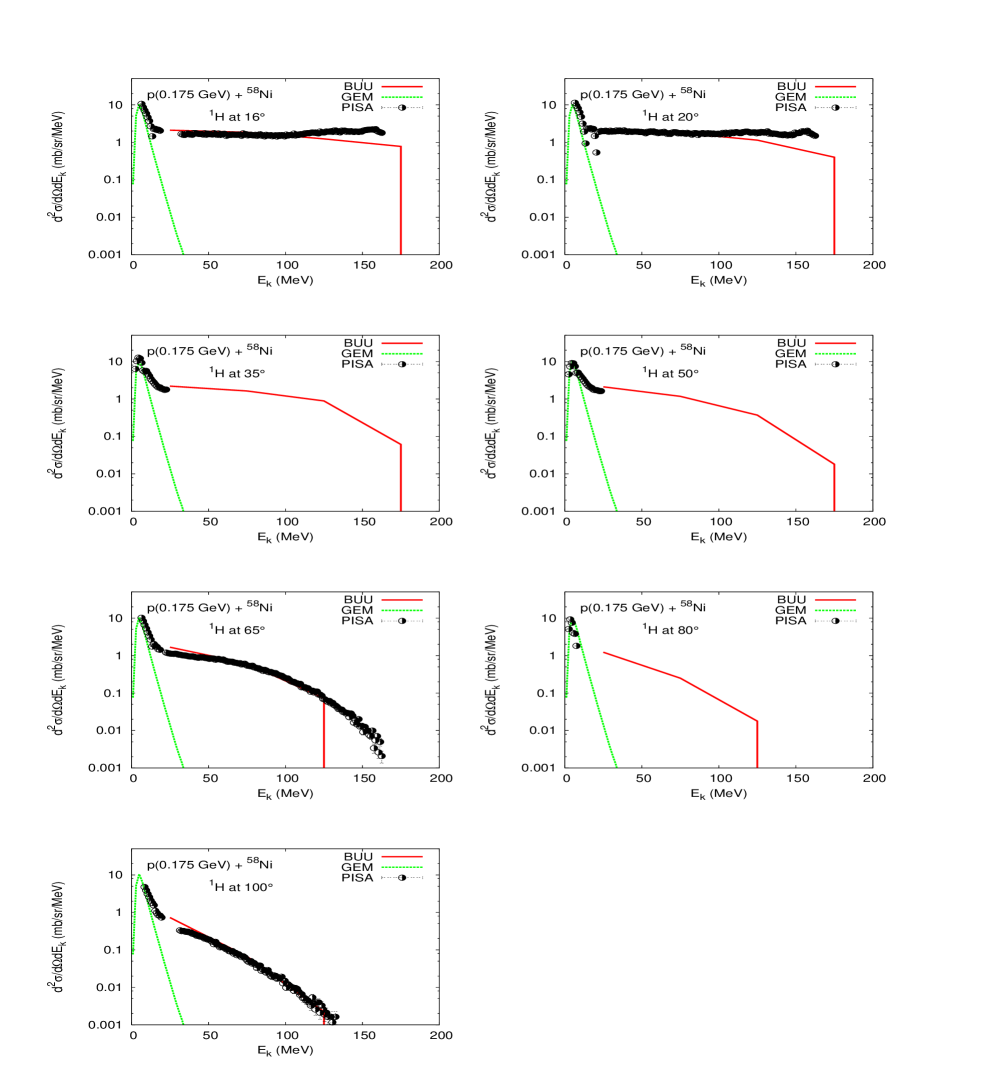
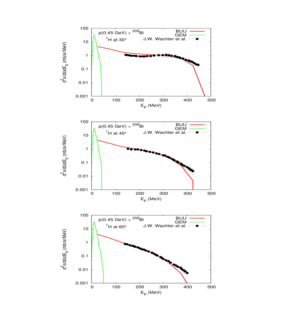
Comparisons of calculated proton spectra produced in reactions induced by higher incident energies, e.g. p+Au at 1.2 GeV, 1.9 GeV and 2.5 GeV projectile energy (with time of first stage calculations equal to 45 fm/c), confronted with data measured by PISA collaboration [7], are shown in Figures 9.13, 9.14 and 9.15. In order to make the comparison easier, the high energy parts of the calculated distributions are plotted only up to 200 MeV of proton kinetic energy. It is seen, that in case of 1.2 GeV of incident energy (Fig. 9.13), the high energy parts of experimental distributions are described well, the low energy parts are slightly overestimated by calculations. In the case of 1.9 GeV beam energy (Fig. 9.14), the whole spectra, especially protons emitted in backward directions are described very well. Low energy part of experimental distributions of protons from reaction at 2.5 GeV (Fig. 9.15) are also very well described by calculations. The high energy parts are slightly underestimated. Nevertheless, the average agreement between the HSD+GEM model results concerning proton spectra and adequate experimental data is satisfactory.
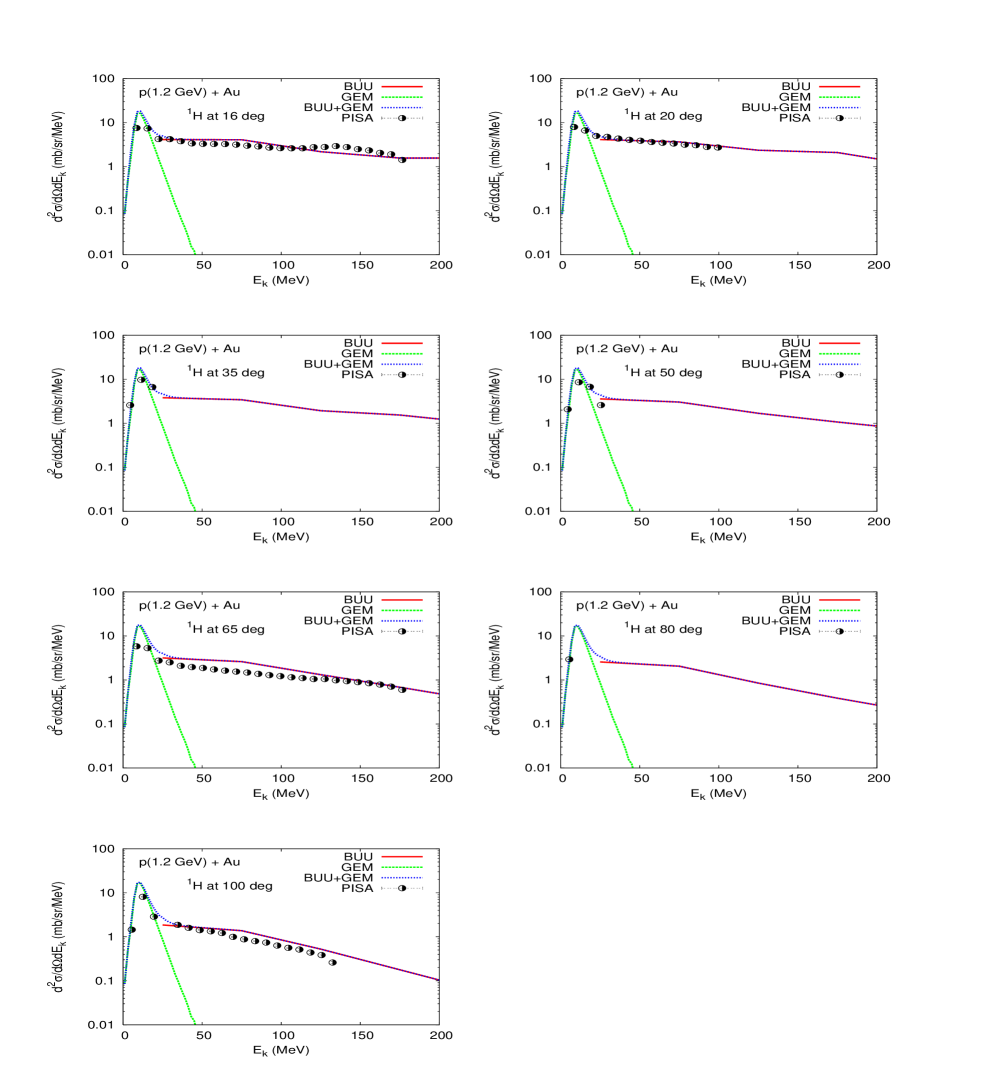
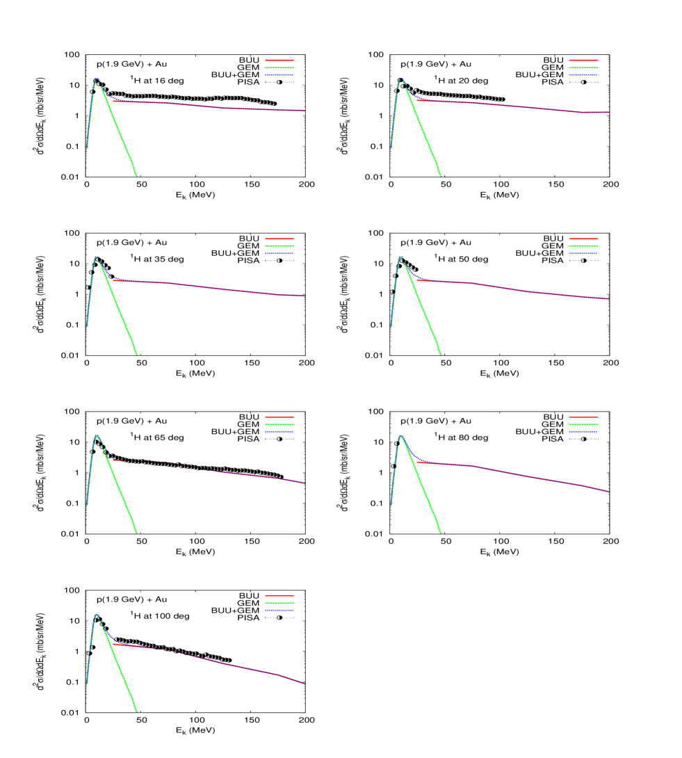

In the presented Figures, contributions from intra-nuclear cascade (high energy part, result of the HSD model calculations) and evaporation (low energy part, result of the GEM model calculations) are visible. The cascade contribution evidently dominates. This indicates, that protons are emitted mainly in the first stage of spallation reaction. This is additionally confirmed by values of multiplicities of protons emitted during first and second stage of reaction, compared in Table 9.2 (quite contrary to the neutron case, consider Table 9.1).
Nucleon distributions depend strongly on projectile energy. The example two-dimensional distributions of transversal () versus longitudinal () momentum of nucleons emitted during the first stage of proton induced reactions on Ni target, at various incident energies are presented in Fig. 9.16. These are results of HSD model calculations, where corresponds to the nucleons momentum in beam direction and is defined as . The two-dimensional distributions depict, how the nucleon spectra evolve with incident energy. In all the cases, low energy part is symmetric around zero value (it is not so in the case of pion production, see Fig. 6.3). With increase of projectile energy, the distribution is building up mainly in longitudinal (forward) direction. It spreads always up to a value corresponding to the value of beam momentum. That is because, it is possible that incoming proton will scatter only slightly on a surface of target nucleus and will appear in forward direction with almost unchanged momentum. In the Fig. 9.16, momentum spectra of all nucleons are presented, since distributions of protons and neutrons emitted during first stage of the reaction are very similar. The only exception concerns momentum corresponding to the beam momentum.
| reaction | first stage | second stage |
|---|---|---|
| p(0.175 GeV)+Ni | 1.61 | 0.91 |
| p(0.45 GeV)+Bi | 2.16 | 1.00 |
| p(1.2 GeV)+Au | 2.67 | 1.13 |
| p(1.9 GeV)+Au | 2.42 | 1.099 |
| p(2.5 GeV)+Au | 2.20 | 0.96 |

9.3 Deuteron spectra
Comparison of inclusive differential energy spectra of deuterons
calculated with the HSD+GEM model, with example experimental data is presented
in Fig. 9.17.

One can see, that only low energy part (i.e. deuterons
evaporated from the residual nucleus during second stage of spallation
reaction) is described by the model calculations. The absence of high energy
part of modelled distributions indicates a lack of deuterons produced during
first stage of the reaction. Certainly, description of the whole distributions
necessitates implementation of some additional mechanisms into the first stage
model. Since deuteron spectra behave very similar as proton distributions
(compare e.g. Figures 9.15 and 9.17), one can
suppose that the high energy part of deuteron spectra are produced due to
a coalescence of proton and neutron during first stage of reaction.
Production of clusters (i.e. light ions) cannot be followed with the HSD
approach, since it is a one body theory.
Nevertheless, a trial of construction of deuterons from the fast
stage of the spallation reaction, with use of informations provided by the HSD
approach, have been undertaken in the frame of this work.
The idea of generation of such deuterons, called here deuterons of
coalescence, is based on the information of positions and momenta of
nucleons belonging to the residual nucleus and nucleons being emitted during
the first stage. The information is taken at a certain point of time, i.e. in
the end of the first stage calculations. Deuterons can be built up in two
manners: by fast proton and proper fast neutron, which are already emitted,
or by
fast proton emitted during fast stage of the reaction and
proper neutron which belongs actually to the excited residual nucleus, but
could have been glued with and taken away by the escaping proton during the
first stage of reaction. In both cases, it is assumed that probability of
creation a deuteron by defined above nucleon pair, depends on their relative
momentum ().
It means, two nucleons are considering as a deuteron if their relative momentum
fulfills assumed condition. The following conditions have been tested:
each pair of neutron and proton can create a deuteron with the same
probability (this gives the highest border of the absolute normalization),
next, deuterons can be created by proton and neutron only if their relative
momentum is lower than or equal to, respectively: 0.45 GeV/c,
0.30 GeV/c and 0.15 GeV/c.
All formed deuterons are additionally repulsed by Coulomb force.
The Coulomb potential is approximated by potential of homogeneously
charged sphere. This is because an incident proton does not cause any
significant changes in the nucleon density distribution inside target nucleus,
as shown in Chapter 4.
Therefore, the kinetic energy of each deuteron is enlarged by value:
| (9.1) |
where: and are charges of target nucleus and deuteron,
respectively, is a radius of target.
Obtained differential energy spectra of deuterons produced in p+Au
reaction at 2.5 GeV proton beam energy are presented in Figures
9.18 and 9.19. The calculated
distributions are compared with experimental data measured by NESSI
collaboration [76].
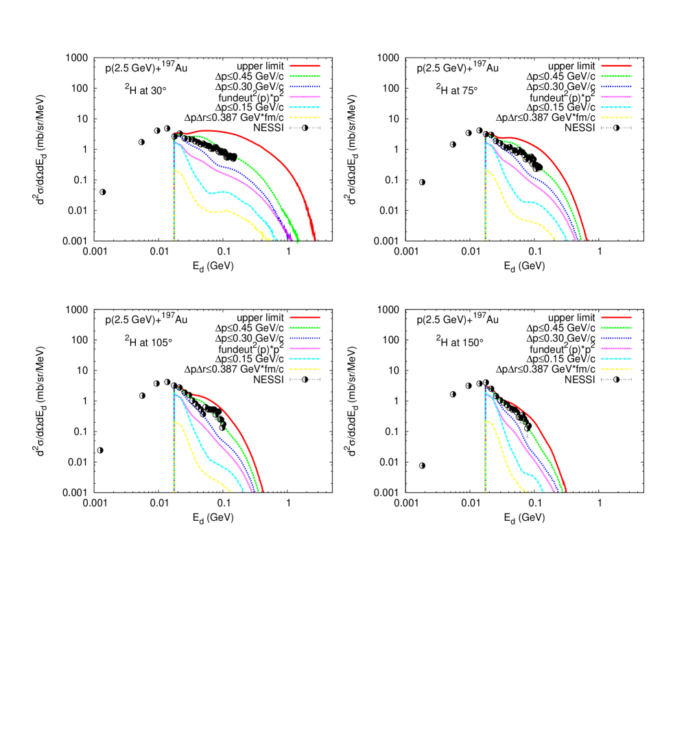
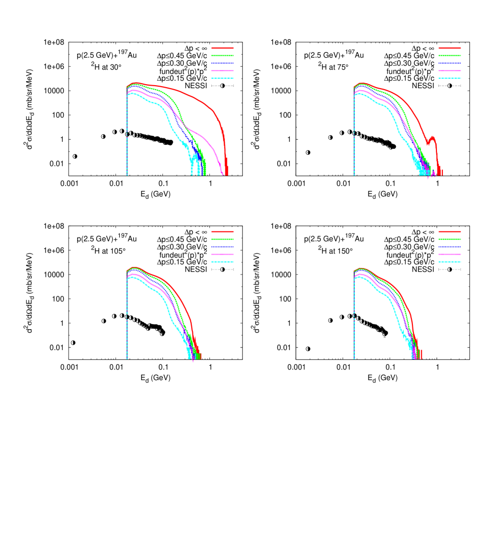
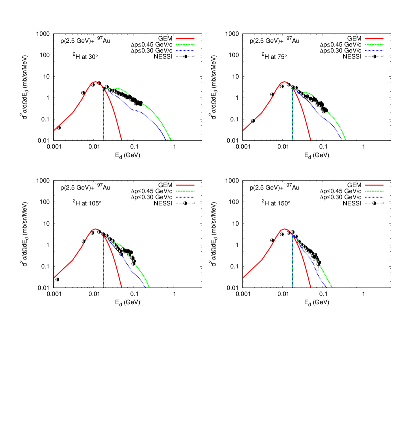
In more precise definition, deuteron is consider as a set of nucleons, which
are sufficiently close to each other in phase space.
Therefore, distributions of deuterons constructed of pairs of fast nucleons,
with condition set not only on their relative momentum (), but also
their relative position () have been tested, too.
The following unit volume of phase space have been selected: 0.387 GeVfm/c (= the Fermi momentum 1.4 fm) [77].
The result underestimates experimental data, as shown in
Fig. 9.18 and 9.19. That is because
of lost of information about the time evolution of relative positions of the
nucleons during the reaction. The condition of relative positions of
nucleons, imposed on the situation at the end of first stage of reaction
rejects nucleon pairs, that it has no record whether in some earlier period of
time nucleons were close enough to create deuterons.
Therefore, it determines, at most, the lowest border of coalescence effect.
There is also possible to define the probability (in fact the density of
probability) of creation a deuteron by a pair of nucleons depending on their
relative momentum, as equal to the modulus of the deuteron
wave function squared: .
The wave function can be parametrized itself as:
| (9.2) |
Values of the coefficients and are taken from
[78]. The used parametrization of the deuteron wave function is
accurate within a few percent, up to momenta of 1 GeV/c,
see Ref. [78].
Obtained in this way spectra of deuterons underestimate the experimental data,
see Figures 9.18 and 9.19.
The calculated spectra of deuterons constructed by two fast nucleons
(Fig. 9.18 and 9.20) are
normalized absolutely. The spectra of deuterons constructed by fast protons and
neutrons from the residual nucleus (Fig. 9.19) cannot be
normalized absolutely.
It is because the information, whether a fast proton before leaving target
nucleus has been near a neutron long enough to
create a deuteron is lost, what gives in this case evident overestimation of
experimental data.
It is seen from the Fig. 9.20, that the high energy part of the experimental spectra are well described by deuterons of coalescence created by a pair of fast nucleons with relative momentum lower or equal to about 0.40 GeV/c. It is also seen that distributions of deuterons of coalescence are perfect continuation of the low energy part. As result, it gives full description of experimental data. However, taking into account shapes of the distributions from Fig. 9.19, one cannot reject possibility that some of the deuterons are produced as coalescence of e.g. fast proton and neutron from residual nucleus.
9.4 Other Ejectiles
Looking at comparison of distributions of heavier particles emitted in proton - nucleus reaction, calculated with the HSD+GEM model with experimental data, displayed in Fig. 9.21, it is seen that only low energy part is described. That is because, in the frame of the model, the light composites are produced only in evaporation stage, as discussed in Sec. 9.3.
It is interesting to know, what is the predictive power of the model, how distributions of the evaporated composites vary with projectile energy and mass of target. Example energy spectra of different ejectiles (isotopes of H, He, Li, Be, B, …) emitted in proton induced reaction on Au target, at a few chosen beam energies are presented in Figures 9.22, and 9.23. Spectra of particles ejected during 2.5 GeV proton induced reactions on few example targets are shown in Figures 9.24 and 9.25. Looking at the distributions of each ejectile, it is clearly seen, that shape of the particular distributions almost does not change with projectile energy, but strongly depends on used target. In all presented cases, the heavier target, the broader the distributions. Average kinetic energy of emitted particle increases with increase of mass of used target, but in this case neutrons are an exception. This indicates, that reason for such behavior is connected with charge of the particles, i.e. Coulomb repulsion force between the ejectiles and an emitting source. The higher charge of the emitting source, the higher average kinetic energy gained by charged ejectiles due to the Coulomb repulsion. Similarly, the particles yield almost does not change with incident energy, but varies significantly with mass of target. Multiplicities of the particles, produced due to discussed here reactions are compared in Tables 9.3 and 9.4. The yield of neutrons increases linearly with increase of the target mass. Multiplicity of each individual charged ejectile varies differently with the target mass. In some cases, it first decreases with the target mass number (for example presented in the Table 9.4, the minimal yield corresponds usually to Ni target) and then increases with further increase of mass of target (e.g. proton yield behaves in opposite way). In many cases, it is also observed roughly linear decrease of the multiplicity with increase of the target mass (as e.g. in case of ). The trends for the particles yield can be to some extent qualitatively understood, since it is known, that the particles emission is influenced by the Coulomb barrier, which is higher for heavier nuclei and by the binding energy, which in average first increases with mass number (A) of target (up to A equal to about 56) and then decreases with A. The relative yield of different ejectiles emitted in one chosen reaction ( Tables 9.3 and 9.4) is also determined by separation energy of individual ejectile, which is not linear with the mass number of ejectile.

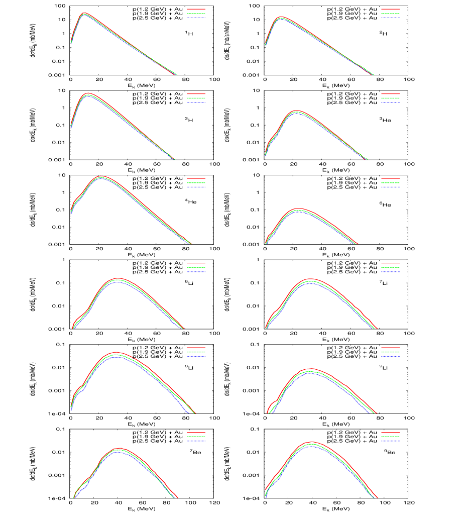
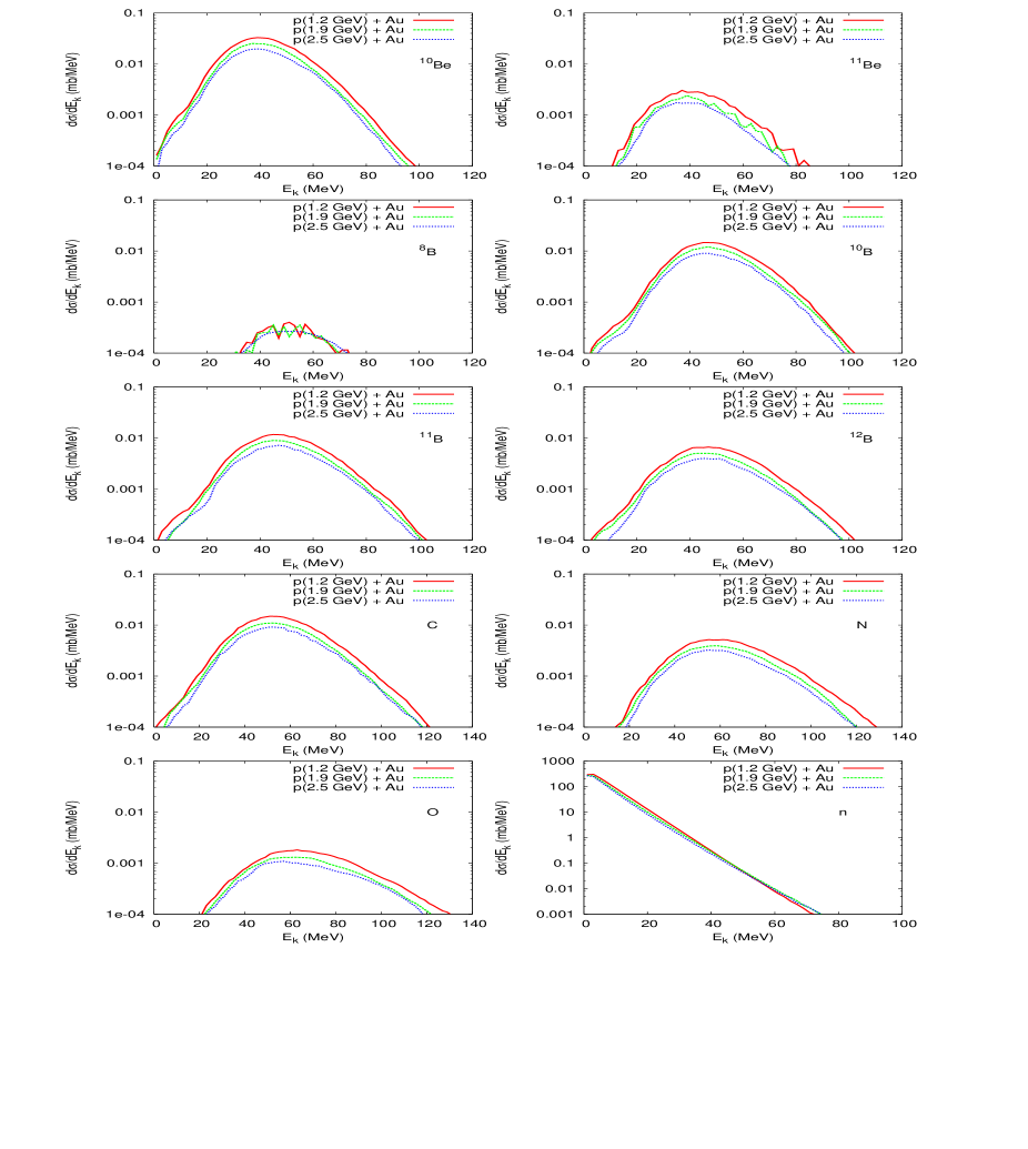
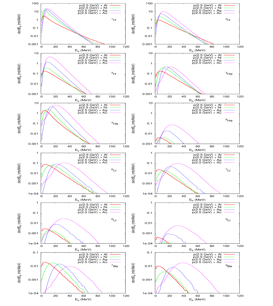
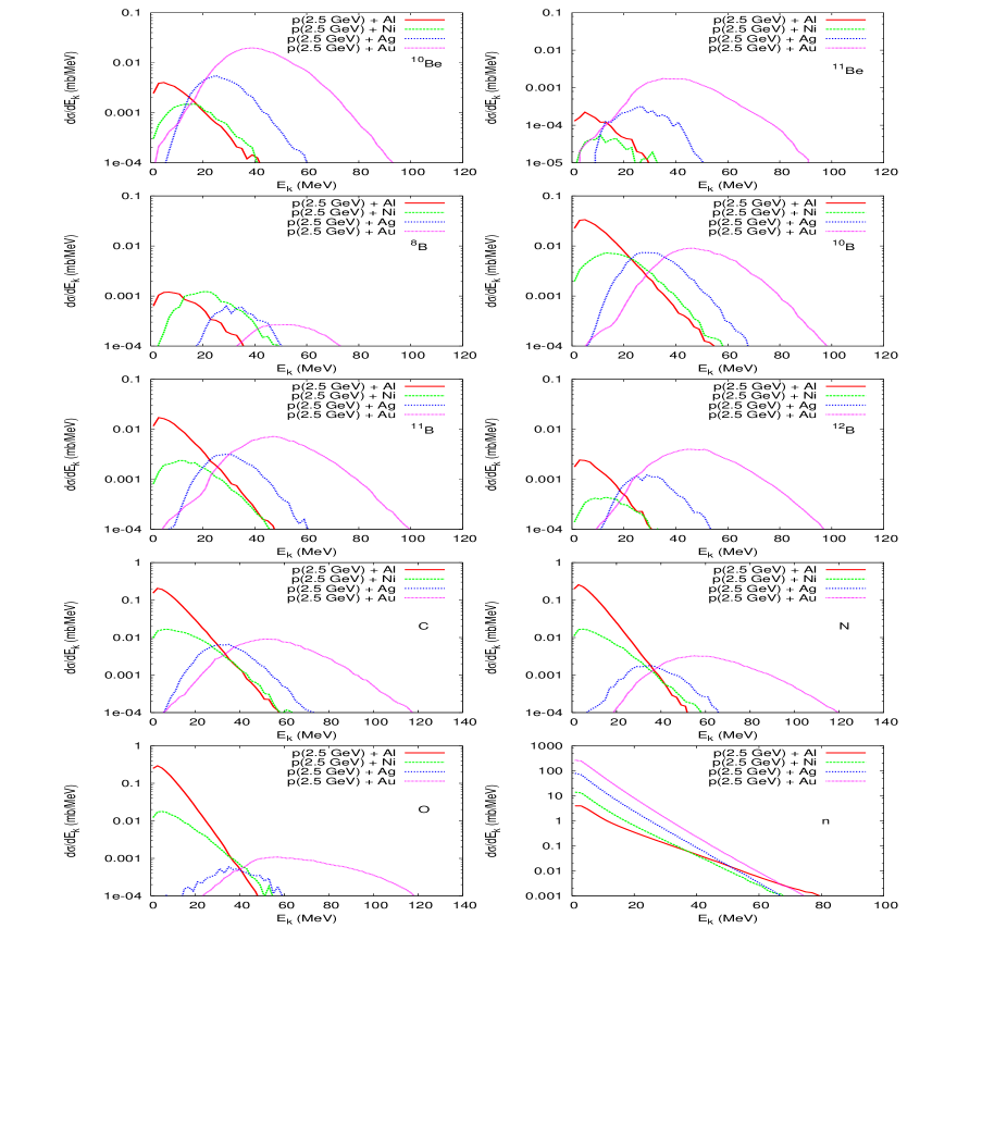
| impact energy | 1.2 GeV | 1.9 GeV | 2.5 GeV |
|---|---|---|---|
| n: | 14.17 | 12.79 | 11.88 |
| : | 1.13 | 1.099 | 0.96 |
| : | 0.59 | 0.59 | 0.51 |
| : | 0.28 | 0.28 | 0.24 |
| : | 0.020 | 0.023 | 0.021 |
| : | 0.59 | 0.56 | 0.48 |
| : | 0.0054 | 0.0058 | 0.0052 |
| : | 0.0045 | 0.0058 | 0.0056 |
| : | 0.0067 | 0.0076 | 0.0067 |
| : | 0.0018 | 0.0022 | 0.0019 |
| : | 0.00039 | 0.00045 | 0.00039 |
| : | 0.00045 | 0.00060 | 0.00055 |
| : | 0.0015 | 0.0017 | 0.0015 |
| : | 0.0018 | 0.0020 | 0.0017 |
| : | 0.00017 | 0.00017 | 0.00016 |
| : | 0.000010 | 0.000018 | 0.000011 |
| : | 0.00065 | 0.00081 | 0.00069 |
| : | 0.00068 | 0.00078 | 0.00067 |
| : | 0.00047 | 0.000497 | 0.00043 |
| : | 0.000061 | 0.000051 | 0.000048 |
| C: | 0.0011 | 0.0012 | 0.0012 |
| N: | 0.00044 | 0.00045 | 0.00043 |
| O: | 0.0002 | 0.00021 | 0.00017 |
| reaction | p+Al | p+Ni | p+Ag | p+Au |
|---|---|---|---|---|
| n: | 0.97 | 1.76 | 6.11 | 11.88 |
| : | 0.82 | 2.20 | 2.19 | 0.96 |
| : | 0.36 | 0.51 | 0.75 | 0.51 |
| : | 0.076 | 0.089 | 0.20 | 0.24 |
| : | 0.082 | 0.10 | 0.082 | 0.021 |
| : | 0.58 | 0.53 | 0.64 | 0.48 |
| : | 0.0017 | 0.0012 | 0.0036 | 0.0052 |
| : | 0.033 | 0.021 | 0.017 | 0.0056 |
| : | 0.0097 | 0.0057 | 0.0092 | 0.0067 |
| : | 0.0012 | 0.00065 | 0.0016 | 0.0019 |
| : | 0.00016 | 0.000046 | 0.00020 | 0.00039 |
| : | 0.0087 | 0.0059 | 0.0032 | 0.00055 |
| : | 0.0040 | 0.0013 | 0.0019 | 0.0015 |
| : | 0.0016 | 0.00055 | 0.0013 | 0.0017 |
| : | 0.000075 | 0.000015 | 0.000068 | 0.00016 |
| : | 0.00059 | 0.00046 | 0.00015 | 0.000011 |
| : | 0.013 | 0.0029 | 0.0019 | 0.00069 |
| : | 0.0061 | 0.00088 | 0.00079 | 0.00067 |
| : | 0.00087 | 0.00016 | 0.00030 | 0.00043 |
| : | 0.000092 | 0.0000069 | 0.000018 | 0.000048 |
| C: | 0.064 | 0.0062 | 0.0018 | 0.0012 |
| N: | 0.070 | 0.0049 | 0.00053 | 0.00043 |
| O: | 0.077 | 0.0048 | 0.00018 | 0.00017 |
| incident energy | after first stage | after second stage |
|---|---|---|
| Tp = 0.5 GeV | 208.361.14 | 188.217.17 |
| Tp = 1.0 GeV | 206.731.48 | 186.657.31 |
| Tp = 2.0 GeV | 205.792.24 | 188.339.70 |
| Tp = 3.0 GeV | 205.702.39 | 189.539.98 |
| Tp = 4.0 GeV | 205.262.82 | 188.6810.24 |
| Tp = 5.0 GeV | 204.573.25 | 187.7010.58 |
| Tp = 7.0 GeV | 203.863.92 | 186.8911.28 |
| Tp = 9.0 GeV | 202.784.73 | 185.0411.83 |
9.5 Massive Fragments
As it is mentioned above, spallation is characterized by observations of one heavy (in respect to the mass of initial target) nucleus, a small number of light fragments and several individual nucleons. Mass distributions of the heavy fragments, produced as result of proton induced spallation reaction on a chosen target vary with incident energy. In Figure 9.26, mass distributions of heavy fragments formed in example p+Pb reactions, at several incident energies (calculated with the HSD + statistical evaporation model), set together with mass distributions of corresponding residual nuclei remaining after first stage of the reactions (results of the HSD model only), are shown.

It is seen, that both of the distributions (after first stage and after whole reaction) broaden with increase of incident energy. Additionally, the higher projectile energy, the lower average mass of nuclei after the first stage of the reaction. Distribution of mass of nuclei produced after the second stage of the reaction is much broader than mass distribution of the remnants of the first stage. The following changes of the distribution of mass of nuclei produced after the second stage, as function of projectile energy are observed. At the lowest presented projectile energy, a maximum at low masses is seen and very small amount of nuclei with masses close to masses of nuclei after first stage of reaction (which are close to mass of the initial target). With increase of incident energy, the distribution broadens. The higher the incident energy, the smaller is the maximum at lower masses. The lighter and lighter nuclei appears. Also more nuclei with masses close to mass of the initial nucleus are produced. Quantitative differences are presented in Table 9.5.
In Figure 9.27, comparison of calculated mass and charge
distributions of products of the proton induced reaction on Au target, at a
few incident energies, with experimental data [79] and [80],
is presented. Agreement between the calculations and measurements is quite
good.
If one compares mass and charge distributions of products of proton induced
reactions on a chosen target, at different projectile energies, significant
difference is seen in mass range and charge range
, as shown in Fig. 9.28.
At the lower projectile energy, two almost separate distributions are visible:
one (, , lower yield) corresponds to fission
products, the second (, , higher yield) indicates
spallation products (fission process is discussed in Sec. 8.2).
At higher incident energy, the split of the distributions vanishes.
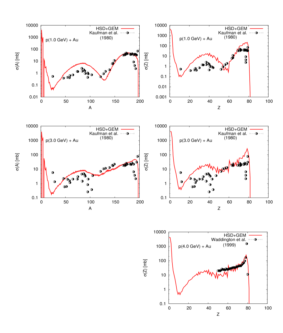
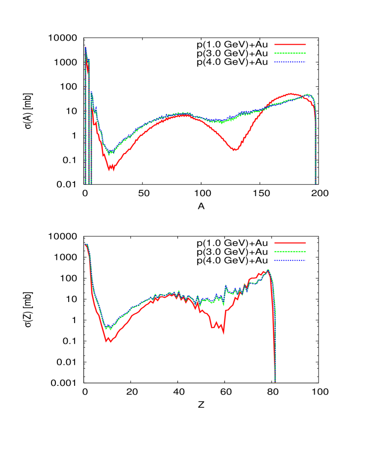
Chapter 10 Comparison of different models predictions on the first stage of proton induced reactions
Apart from the HSD model, a few other microscopic models have been developed in order to describe the fast stage of proton - nucleus reaction. All the models are based on different assumptions or simplifications (as described in Chapters 2 and 3). It is interesting to compare their predictions. In this chapter, results of the HSD, INCL4 ([17]) and QMD ([19]) models are examined.
The most important issue for comparison of results of various models of the first stage of proton - nucleus reaction are: particles production during the first stage of the reaction and properties of residual nuclei remaining after the stage. Predictions on pion production are particularly interesting for comparison. This is due to the fact, that calculations of the first stage of reaction are sufficient in order to receive realistic pion spectra, as all pions are produced only in the fast cascade of nucleon - nucleon collisions, where the available amount of four-momentum is large enough. One of the important features which can influence the magnitude of pion production and absorption is treatment of the nucleon-nucleus mean field (that corresponds to the main difference between the models). To check whether assumptions concerning the mean field in the model calculations affect significantly multiplicity of produced pions, results of the HSD model are compared with the INCL4 and QMD models calculations and presented in Tables 10.1 and 10.2, for 2.5 GeV proton induced reactions on Ni and Au target, respectively.
| HSD | INCL4 | QMD | |
|---|---|---|---|
| 0.51 | 0.35 | 0.42 | |
| 0.46 | 0.34 | 0.36 | |
| 0.38 | 0.18 | 0.28 |
| HSD | INCL4 | QMD | |
|---|---|---|---|
| 0.49 | 0.29 | 0.34 | |
| 0.53 | 0.35 | 0.34 | |
| 0.46 | 0.25 | 0.32 |
It is seen that the relative behavior of the pion multiplicities obtained from the different models is similar: for lighter target (Ni) the : : ratio is equal to 1 : 0.86 : 0.67 for QMD [82], 1 : 0.97 : 0.51 for INCL4 [81] and 1 : 0.90 : 0.75 for the HSD, while for the heavy target (Au) 1 : 1 : 0.94 (QMD [82]), 1 : 1.21 : 0.86 (INCL4 [81]) and 1 : 1.08 : 0.94 (HSD). However, absolute values of pion multiplicities obtained from the HSD model are always higher by factor 1.5 than the values received from the INCL4 and the QMD models, although results of the HSD model are closer to that of the QMD model.
Let’s compare now also an amount of kinetic energy carried out by the most abundantly produced particles during the first stage of the reaction, i.e. nucleons and pions. The average multiplicity and average kinetic energy of nucleons and pions emitted during the first stage of example 2.5 GeV proton induced reaction on Au target are displayed in Table 10.3.
| HSD | INCL4 | QMD | ||||
|---|---|---|---|---|---|---|
| n | 2.23 | 0.781.27 | 3.48 | 0.801.46 | 7.63 | 0.761.83 |
| p | 2.20 | 0.901.36 | 2.68 | 0.961.58 | 5.63 | 0.962.31 |
| 0.49 | 0.140.13 | 0.25 | 0.070.08 | 0.32 | 0.090.11 | |
| 0.53 | 0.150.15 | 0.35 | 0.130.13 | 0.34 | 0.100.12 | |
| 0.46 | 0.130.13 | 0.29 | 0.110.11 | 0.34 | 0.110.12 | |
The values collected in Table 10.3 indicate, that although the average multiplicity of emitted particles provided by the models are slightly different, the average amount of kinetic energy carried out by the particles is almost identical in all of the models. Consequently, properties of residual nuclei evaluated by the different models should be similar. In Figure 10.1, comparison of the properties of residual nuclei, i.e. distributions of mass, charge, excitation energy and momentum in beam direction of the residual nucleus created in example p+Au reaction, at 2.5 GeV beam energy, are shown. The adequate average values are listed in Table 10.4. One observes that the HSD and INCL4 predictions are quite similar.

| HSD | INCL4 | QMD | |
|---|---|---|---|
| 193.03.3 | 191.84.03 | 183.510.1 | |
| 77.61.8 | 77.31.9 | 73.84.3 | |
| 201.7171.3 | 253.6226.3 | 195.5165.8 | |
| 0.280.35 | 0.440.51 | 0.580.62 |
Results of the models are sensitive to used parameters
(in particular time duration of the first stage calculations, which is
determined for each model individually, see [17, 19]).
Therefore it is worthy to compare results obtained from each of the model and
estimate their predictive power by confrontation with experimental data.
In order to describe the nuclear reaction in unified way to verify predictions
of the different models with experimental observations, the first
stage models have been incorporated with one chosen statistical evaporation
model applied for the second stage of reaction, i.e. GEM [21].
Output of the HSD, INCL4 and QMD model, respectively (i.e. mass, charge,
momentum and excitation energy of the residual nuclei) defines input for the
GEM model.
In order to verify which of the distributions of the properties displayed in
the Fig. 10.1 is the most reliable, calculated
double differential kinetic energy spectra of 4He emitted at two different
angles during p+Au reaction at 2.5 GeV incident energy are compared with
experimental data [7], and shown in Fig.
10.2. Distributions of 4He
are the best choice for such a comparison due to the fact, that in the
4He channel evaporation is dominant. As it is shown in Ref.[7],
about 90 of the 4He spectrum consists of the particles produced
during the evaporation stage. One can see, that the models give similar
results, although the HSD and the QMD model results are somehow closer to
experimental data.
In Figure 10.3, comparison of calculated example
fragment mass and charge distributions compared with experimental data
[79] and [80] are displayed.
It is seen, that also in this case the models give similar results.
In particular, results of the HSD and the INCL4 models are almost identical.
If looking at the QMD model calculations, plotted for reaction p+Au at 1.0
GeV beam energy, in the emitted fragment mass number and charge range
corresponding to the fission peak (i.e. and ), they are
lower than calculations of the other models, but closest to the
experimental data. However, outside the range (i.e. , and ,
) results of all considered here models are very similar.


Based on the comparisons, one can conclude that results of the HSD model do not differ significantly from results of the other models. The additional verification by confrontation of the calculations with experimental data indicates, that results of the HSD and the QMD model are particularly close to the experimental data. As results of the HSD model are not distinctly different from that of the QMD model (which is actually the most advanced one), a big advantage of the HSD model, connected with respectively short time of calculations should be mentioned. The average time needed to calculate a reaction with the QMD model is of the order of a few days, while time needed to calculate the adequate reaction with the HSD model - only few hours.

Chapter 11 Summary and Conclusions
Global information of properties of proton - nucleus reactions
(i.e. particles production, properties of residual nuclei after
first stage of the reactions) has been presented in wide range of projectile
energy and mass of target nuclei, with the Hadron String Dynamics (HSD)
[38, 39] model for the first stage of the reaction,
incorporated with statistical evaporation model (GEM [21] and PACE2
[20]) for the second stage. It has been confronted with experimental
data and results of other models.
The version of the HSD code [38] has been developed in order to
describe proton induced spallation reactions in wide energy range
in the following aspects. First of all, to calculate properties of residual
nuclei after first stage of the reaction, defining an input for
models of the second stage calculations.
The code has been developed for description of pion production
in proton - nucleus reactions.
Additionally, a version of HSD code that allows for calculations of pion
induced reactions has been prepared.
Stopping time for the first stage model calculations has been established
based on behaviors of excitation energy, longitudinal momentum and angular
momentum as a function of time. These are decisive for determination of the
duration time of the first stage of proton - nucleus collisions, due to the
fact that in the dependences two phases can be distinguished: a phase of rapid
variations, followed by a phase of much slower variations, indicating
thermodynamical equilibrium of the nucleus. Properties of residual nuclei are
evaluated by exploring conservation of energy, mass, charge, momentum and
angular momentum.
It has been shown, that distributions of properties of residual nuclei (i.e. mass, charge, excitation energy, momentum, angular momentum) differ significantly with mass of target, but behave similarly for varied projectile energies. Multiplicity of emitted pions increases with incident energy and with target mass number. Contrary, e.g. average kinetic energy of other individual emitted particles (i.e. nucleons, pions) increases with kinetic energy of incoming proton, but decreases with target mass number. Higher nucleon and pion momenta and their increasingly forward peaked distributions are associated with increasing incident energy. That is connected with increasingly forward focused nature of nucleon - nucleon collisions with increase of incident energy; the total nucleon - nucleon scattering cross section remains approximately constant, but ratio of inelastic to elastic collisions increases rapidly with impact energy [45].
It has been shown, that the biggest amount of initial energy deposited in nucleus by incoming proton is carried out during the first stage of the reaction, i.e. about 85 , and only about 15 of the initial energy is carried away during the second stage of the reaction. Most of the initial energy is carried out by nucleons and pions. Neutrons are emitted mainly in the second stage of reaction, whereas protons - mainly during the fast cascade stage. Pions are emitted only in the first stage of reaction, where the locally available amount of four-momentum is large enough. In case of light composites, only low energy part of distribution, corresponding to a result of evaporation stage, is described by the HSD plus evaporation model. E.g. for deuterons, the absence of high energy part of modelled distributions indicates a lack of deuterons produced during first stage of the reaction. Description of the whole distributions necessitates future implementation of some additional mechanisms into the first stage model, e.g. coalescence processes. It is observed already in neutron spectra that these additional mechanisms have to depend strongly on size of the system: for heavier targets the neutron spectra in some region are visibly underestimated by model calculations, see Fig. 9.10.
Very interesting conclusion of the work is a prevision for a negligible probability for fragmentation in proton induced reactions, at considered here range of incident energy. This statement is based on results of the HSD model calculations of excitation energy per nucleon of residual nuclei and time evolution of nucleon density. Results of the HSD model show, that a value of excitation energy greater than 5 MeV/N occurs very rarely, in only few percent of cases (studies of fragmentation have found that it occurs at a value of excitation energy per nucleon of a residual nuclei at least equal to about 5 MeV/N [54, 55]). Fragmentation could be more probable if a part of nuclei takes part in excitation, i.e. the excitation energy should be calculated only per some amount of the active nucleons; only this part of nucleus would undergo fragmentation. However modelling of nucleon density evolution with the reaction time shows, that proton induced reactions are very low - invasive processes. Incoming proton causes insignificant modifications of the nuclear density. Energy is rather uniformly distributed among the nucleons of residual nuclei. A situation, when two differently excited parts of nucleus appear, occurs only in about of proton - nucleus reaction cases and rather in peripheral collisions, whereas experimentalists associate fragmentation with central collisions.
It has been shown that in proton induced reaction, in the considered here incident energy range, spallation is evidently dominant process. Moreover, the second stage of spallation reaction is a competition between evaporation and fission.
Results of the HSD model calculations have been compared with available experimental data and with adequate results of other microscopic models (i.e. INCL4 [17] and QMD [19]). The comparisons model - model show that results of the HSD model do not differ significantly from results of the other models calculations. Results of the HSD model are also consistent with various experimental data. Qualitatively, the data are well described by the calculations. Quantitatively, the maximal noticed discrepancy is of factor 2. It concerns pion spectra, which are the worst described cases, i.e. overestimated by a factor of 2. That is because, despite description of NN interactions is well established, details of pions propagation in nuclear matter are very delicate. Legth of free path for pions in nuclear matter of standard density is 1 - 1.5 fm. It means, pions that arrive to detectors stem from surface of nucleus. In models like HSD it is just the surface that is described only approximately. Pions production due to proton - nucleus collisions is a complicated process, since they are not emitted directly, but result from a succession of productions and absorptions inside a nucleus, mediated by Delta resonance.
The comparisons indicates that assumptions and simplifications employed in the HSD model are correct.
In order to obtain the possible best description of proton induced reactions, trials of various feasible modifications of the HSD model parameters has been investigated. However, the possible modifications, as in case of each of semi-classical models are limited. A necessity of the exact fully quantum model appears. Unfortunately, construction of such model of many body strongly interacting system is at present practically impossible.
Summarizing, the global properties of proton induced reactions have been presented in wide range of mass of target and incident energy. It has been shown, that these are quite non-invasive reactions, where spallation is the dominant process. Properties of residual nuclei after the first stage of the reaction are weakly dependent on incident energy, but strongly dependent on mass of target. High momenta of emitted particles are associated with high incident energies. The second stage of the reaction is a competition of evaporation and fission. The agreement of results of the HSD calculations with experimental data and with results of the other microscopic models calculations indicates that proper assumptions have been employed in the HSD model. As discussed in Sec. 5.1, results obtained from the HSD model vary smoothly as function of proton incident energy and mass of target, so interpolation of results is quite feasible.
Acknowledgments
I would like to thank all the people who helped me during the years of
Ph. D. studies.
First of all I would like to express my enormous gratitude to Dr hab. Zbigniew Rudy, for devoting his time, many ideas that helped to bring this dissertation into existence, for his guidance, patience, support, encouragement and help whenever I need it.
I am grateful to Prof. Bogusław Kamys for allowing me to prepare this dissertation in the Faculty of Physics, Astronomy and Applied Computer Science of the Jagiellonian University.
I am extremely grateful to Prof. Bogusław Kamys and Prof. Lucjan
Jarczyk for giving me an opportunity to work in PISA collaboration.
I am indebted to them for their helpful ideas, suggestions, their kindness,
support and encouragement during all the years of my studies.
A big ”thank you” to all colleagues from the PISA collaboration,
especially to:
Prof. D.Filges, Dr F.Goldenbaum, Prof. L.Jarczyk, Prof. B.Kamys, Dr M.Kistryn,
Dr hab. St.Kistryn, Dr E.Kozik, Prof. A.Magiera, B.Piskor-Ignatowicz,
M.Puchała, Dr K.Pysz, Dr hab. Z.Rudy
and M.Wojciechowski.
I’d like to express my gratitude to Dr Małgorzata Kistryn and Małgorzata Puchała for communication concerning results of INCL and QMD model calculations.
I would like to acknowledge Prof. Ulrich Mosel for allowing me to work in his group, at the Institut of Theoretical Physics of Justus-Liebig University in Giessen.
I am extremely grateful to Prof. Wolfgang Cassing for giving me an opportunity to work under his guidance at the Institut of Theoretical Physics in Giessen and ability to use his HSD code. I am indebted to him for help in developing of the code, for sharing his experience, devoting his time and for his patience.
I would like to acknowledge Prof. Jim Ritman for allowing me to work in Research Center Juelich.
I am grateful to Dr Frank Goldenbaum, for the invitation to the Research Center Juelich, for his kindness and help.
I am very grateful to Dr hab. Zbigniew Rudy for careful reading and correcting
this dissertation.
I am also very grateful to Prof. Bogusław Kamys, Prof. Lucjan Jarczyk and
Dr Frank Goldenbaum for correcting some parts of this thesis.
Thanks to all my colleagues from ”the room 03A”, from Giessen and from IKP for the pleasant atmosphere of the daily work.
Bibliography
- [1] N. Bohr, Nature 137(1936)344
- [2] B. B. Cunningham et al., Phys. Rev. 72(1947)739
- [3] R. Serber, Phys. Rev. 72(1947)1114
- [4] V. Weisskopf, Phys. Rev. 52(1937)295
- [5] N. Metropolis et al., Phys. Rev. 110(1958)185
- [6] I. Dostrovsky et al., Phys. Rev. 111(1958)1658
- [7] A. Bubak et al., Non-equilibrium emission of complex fragments from p+Au collisions at 2.5 GeV proton beam energy, accepted for publication in Phys. Rev. C, 2007.
- [8] F. Goldenbaum et al., Phys. Rev. Lett. 77(1996)1230
- [9] W. Przygoda et al., Nucl. Phys. A 783(2007)583
- [10] S. Aiello et al., Nucl. Phys. A 583(1995)461
- [11] B. S. Brown, A. D. Taylor, ICANS XIII, 13th Meeting of the International Collaboration on Advanced Neutron Sources, Report PSI-Proc. 95-02, November 1995, ISSN 1019-6447
- [12] R. Pynn, ICANS XI, 11th Meeting of the International Collaboration on Advanced Neutron Sources, Report KEK 90-25
- [13] G. S. Bauer, ICANS XIV, 14th Meeting of the International Collaboration on Advanced Neutron Sources, Report ANL-98/33, ISSN 1560-859X
- [14] C. D. Bowman et al., Nucl. Inst. Meth. in Phys. Res. A 320(1992)336
- [15] R. Silberberg, C. H. Tsao, Phys. Rep. 191(1990)351
- [16] S. G. Mashnik, On Solar System and Cosmic Rays Nucleosynthesis and Spallation Processes, LANL, Report LA-UR-00-3658, (2000)
- [17] J. Cugnon et al., Nucl. Phys. A, 620(1997)475
- [18] K. Niita, W. Cassing and U. Mosel, Nucl. Phys. A, 504(1989)391
- [19] J. Aichelin, Phys. Rep. 202(1991)233
- [20] A. Gavron in Computational Nuclear Physics 2, Nuclear Reactions, edited by K. Langanke et al., Springer-Verlag 1993, p. 108
- [21] S. Furihata, Nucl. Inst. Meth. in Phys. Res. B 171(2000)251
- [22] H. W. Bertini, Phys. Rev. 131(1963)1801
- [23] Y. Yariv and Z. Fraenkel, Phys. Rev. C, 20(1979)2227
- [24] K. Niita et al., Phys. Rev. C 52(1995)2620
- [25] E. Wigner, Phys. Rev. 40(1932)749
- [26] J. Cugnon et al., Nucl. Phys. A 352(1981)505
- [27] J. Richert, P. Wagner, Phys. Rep. 350(2001)1-92
- [28] W. Bauer, D. R. Dean, U. Mosel, U. Post, Phys. Lett. B, 150(1985)53
- [29] W. Bauer, U. Post, D. R. Dean, U. Mosel, Nucl. Phys. A, 452(1986)699
- [30] X. Campi and J. Desbois, in Proceedings of the 23rd Bormio Conference (Ricerca Scientifica ed Educatione Permanente, Milano, 1985), p. 497
- [31] W. Bauer, Phys. Rev. C, 38(1988)1297
- [32] A. S. Hirsch et al., Phys. Rev. C, 29(1984)508
- [33] T. Murakami et al. (MULTI collab.), Proc. of the Int. Symp. on Clustering Aspects of Quantum Many-body Systems (World Scientific, 2002), p.177
- [34] D. R. Fortney et al., Phys. Rev. C, 21(1980)2511
- [35] Y. Hirata et al., nucl-th/0111019
- [36] S. Yamaguchi and A. Ohnishi, Prog. Theor. Phys. 156(2004)150
- [37] G. F. Bertsch and S. Das Gupta, Phys. Rep. 160(1988)189
- [38] W. Cassing, private communication
- [39] J. Geiss, W. Cassing, C. Greiner, Nucl. Phys. A, 644(1998)107
- [40] B. Anderson, G. Gustafson, Hong Pi, Z. Phys. C, 57(1993)485
-
[41]
Donald H. Perkins, Introduction to High Energy Physics,
(University Press, Cambridge, 2000) - [42] B. Anderson, G. Gustafson, G. Ingelman, T. Sjoestrand, Phys. Rep. 97(1983)31
- [43] A. E. Uehling and G. E. Uhlenbeck, Phys. Rev. 43(1933)552
- [44] G. F. Bertsch, H. Kruse and S. Das Gupta, Phys. Rev. C, 29(1984)673
- [45] Particle Data Group, Phys. Rev. D, 50(1994)1173
- [46] J.H. Koch et al., Ann. Phys. 154(1984)99
- [47] S. Teis et al., Z. Phys. A 356(1997)421
- [48] J. Geiss, PhD thesis, 1998, not published
- [49] W. Cassing, E.L. Bratkovskaya, U. Mosel, S. Teis and A. Sibirtsev, Nucl. Phys. A, 614(1997)415
- [50] W. Ehehalt and W. Cassing, Nucl. Phys. A, 602(1996)449
- [51] J. Geiss, C. Greiner, E. L. Bratkovskaya, W. Cassing, U. Mosel, nucl-th/9803008
- [52] A. Strzałkowski, Wstȩp do fizyki ja̧dra atomowego, W-wa 1979, PWN
- [53] A. Bubak, B. Kamys, M. Kistryn, B. Piskor-Ignatowicz, Nucl. Instr. Meth. B 226(2004)507
- [54] L. Beaulieu et al., Phys. Rev. Lett. 84(2000)5971
- [55] V. E. Viola et al., Phys. Rep. 434(2006)1
- [56] J.Martensson et al., Phys. Rev. C 62(2000)014610
- [57] D. R. F. Cochran et al., Phys. Rev. D 6(1972)3085
- [58] A. Boudard et al., Phys. Rev. C 66(2002)044615
- [59] Baldini et al.: Landolt-Boernstein vol. 12, Springer, Berlin (1987)
- [60] Th. Aoust and J. Cugnon, Phys. Rev. C 74(2006)064607
- [61] A. Engel et al., Nucl. Phys. A 572(1994)657
- [62] A. Kowalczyk, Diploma Thesis, Jagiellonian University 2002, not published
- [63] W. Hauser and H. Feshbach, Phys. Rev. 87(1952)366
- [64] J. R. Grover, Phys. Rev. 127(1962)2142
- [65] A. Bohr and B. R. Mottelson, Struktura Ja̧dra Atomowego, W-wa 1957, PWN
- [66] A. J. Sierk, Phys. Rev. C, 33(1986)2039
- [67] C. M. Perey and F. G. Perey, At. Nucl. Data Tables 17(1976)1
- [68] J. R. Huizenga and G. Igo, Nucl. Phys. 29(1962)462
- [69] V. Weisskopf and P. Ewing, Phys. Rev. 57(1940)472
- [70] I. Dostrovsky et al., Phys. Rev. 116(1959)683
- [71] A. Gilbert and A.G.W. Cameron, Can. J. Phys. 43(1965)1446
- [72] H. G. de Carvalho et al., Nucl. Phys. 53(1964)345
- [73] S. Leray et al., Phys. Rev. C, 65(2002)044621
-
[74]
S. Meigo et al., Nucl. Instr. Meth. A 431(1999)521
K. Ishibashi et al., J. Nucl. Sci. Technol. 34(1997)529 - [75] J. W. Wachter et al., Phys. Rev. C 6(1972)1496
- [76] A. Letourneau et al., Nucl. Phys. A, 712(2002)133
- [77] A. Boudard et al., Nucl. Phys. A, 740(2004)195
- [78] G. Alberi, L. P. Rosa, Z. D. Thome, Phys. Rev. Lett., 34(1975)503
- [79] S. B. Kaufman and E. P. Steinberg, Phys. Rev. C 22(1980)167
- [80] C. J. Waddington et al., The Astrophysical Journal, 519(1999)214
- [81] M. Kistryn, private communication (2007)
- [82] M. Puchała, private communication (2007)