Resonant Inelastic X-ray Scattering (RIXS) Spectra for Ladder Cuprates

Abstract

The ladder compound Sr₁₄Cu₂₄O₄₁ is of interest both as a quasi-one-dimensional analog of the superconducting cuprates and as a superconductor in its own right when Sr is substituted by Ca. In order to model resonant inelastic x-ray scattering (RIXS) spectra for this compound, we investigate the simpler SrCu₂O₃ system in which the crystal structure contains very similar ladder planes. We approximate the LDA dispersion of SrCu₂O₃ by a Cu only two-band tight-binding model. Strong correlation effects are incorporated by assuming an anti-ferromagnetic ground state. The available angle-resolved photoemission (ARPES) and RIXS data on the ladder compound are found to be in reasonable accord with our theoretical predictions.

I Introduction

Resonant inelastic x-ray scattering (RIXS) is a second-order optical process in which there is a coherent absorption and emission of X-rays in resonance with electronic excitations.KoShin RIXS can probe charge excitations extending to fairly high energies of up to $\sim$ 8 eV. This allows the analysis of electronic states over a wide energy range, including electron correlation effects originating from strong electron-electron Coulomb repulsion, providing thus a powerful tool for investigating Mott physics in solids.

The chain-ladder compound Sr₁₄Cu₂₄O₄₁ exhibits very interesting magnetic, transport and properties. It has attracted wide attention due to the discovery of a superconducting phase in highly Ca-doped samples at high pressure nagata and charge order of the doped ladder abbamonte . The compound possesses an incommensurate layered structure consisting of alternating layers of sublattices involving CuO₂ chains and Cu₂O₃ ladders. The superconductivity arises on the ladders, making them a quasi-one-dimensional analog of the cuprates. Very recently, K-edge RIXS data on the ladder compound has been reportedHasan ; Ishii , providing motivation for undertaking corresponding theoretical modeling of the spectra. Here, we attempt to do so by considering the simpler analog compound SrCu₂O₃. This should be a good approximation since interlayer coupling in Sr₁₄Cu₂₄O₄₁ is negligible arai , and both compounds have very similar ladder planes with similar hopping parameters muller . Specifically, we obtain K-edge RIXS spectra within a mean field approach for momentum transfer along as well as perpendicular to the direction of the ladders. A two-band Cu-only tight-binding model is used in which strong correlation effects are incorporated by treating an antiferromagnetic (AFM) ground state.

II Electronic Structure and the Two Band Model

The spin-ladder compound SrCu₂O₃ possesses the orthorhombic structure with space group Cmmm in which Cu₂O₃ planes are stacked with Sr atoms sandwiched between these planes.John Fig. 1 shows the detailed arrangement of Cu and O atoms in the Cu₂O₃ planes. This so-called ‘trellis structure’ involves Cu-O ladders where successive ladders are seen to be offset by half a unit cell. We obtained the band structure of SrCu₂O₃ self-consistently using a full-potential, all electron scheme within the local density approximation (LDA)wien2k ; bansil99_1 . The first principles bands were fitted by a 2-band tight-binding (TB) model in the vicinity of the Fermi energy, and provided the basis for RIXS computations presented in this study. Fig. 2 shows the first-principles as well as the TB bands along several high symmetry lines in the Brillouin zone (BZ). There are seen to be only two bands around the Fermi energy, which display large dispersion along the ladder direction $\Gamma$-Z, and a relatively smaller dispersion along the perpendicular $\Gamma$-X direction. In the first-principles band structure, both these bands are dominated by states of Cu $d_{x^{2}-y^{2}}$ character whose weight is given by the color bar on the right hand side of Fig. 2.

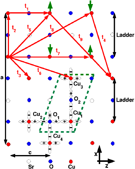
Figure 1: (color online) Arrangement of Cu and O atoms in the Cu₂O₃ planes in the form of a series of ladders offset by half a unit cell along the c-axis. Unfilled circles give the location of out-of-plane Sr atoms. The green parallelepiped marks a primitive unit cell around which the orientation of Cu $d_{x^{2}-y^{2}}$, O ${p_{x}}$, and O ${p_{y}}$ orbitals is shown. Red arrows give the specific hopping parameters used in two-band model fits to the band structure. The AFM ordering of spins in the ladders is depicted by the green arrows.

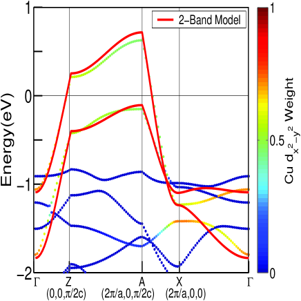
Figure 2: (color online) First-principles LDA band structure of SrCu₂O₃ along several high symmetry lines in the irreducible Brillouin zone is shown by dots of various colors. The colors of the dots code the weight of Cu $d_{x^{2}-y^{2}}$ character in the associated wavefunctions as indicated by the color-bar on the right hand side of the figure. Solid red lines give the 2-band tight-binding model fit to the LDA bands near the Fermi energy.

In making a TB fit to the two aformentioned LDA bands near the Fermi energy, we have adapted a Cu-only 2-band model suggested in Ref. muller, . The detailed form of the TB Hamiltonian is discussed in the Appendix. The TB bands are seen from Fig. 2 to provide a good fit to the LDA bands near the Fermi energy. Our values of various parameters, i.e. the on-site energy $\epsilon_{0}$ and the hopping parameters $t_{1}-t_{9}$, are seen from Table 1 to be in reasonable accord with those of Ref. muller, . The meaning of specific overlap terms involved in defining $t_{1}-t_{9}$ is clarified by the red arrows in Fig.  1. The present TB model includes not only the nearest neighbor hopping terms $t_{1}-t_{3}$, but also the longer range hoppings $t_{4}-t_{9}$. Interestingly, we find that the inter-ladder dispersion (i.e. along Z-A in Fig. 2) cannot be fitted well using only a nearest-neighbor hopping model. Table 1 shows that the intra-ladder hopping parameters ($t_{1}$, $t_{2}$ and $t_{5}$) are generally larger than the inter-ladder terms such as $t_{3}$, $t_{4}$ and $t_{6}$. This can be understood with reference to Fig. 1 where orientation of the Cu-$d_{x^{2}-y^{2}}$ and O-$p_{x}$ and $p_{y}$ orbitals is sketched on a few sites. An intra-ladder Cu-O-Cu path with a bond angle of $180^{o}$ (e.g. Cu₂-O₁-Cu₁) will be expected to provide a larger orbital overlap than an inter-ladder path with a $90^{o}$ bond (e.g. Cu₄-O₁-Cu₁). The glide symmetry of SrCu₂O₃ leads to some dispersion anomalies, including extra degeneracies at the zone boundaries and an apparent $4\pi$ periodicity of the dispersion along the ladder. A $2\pi$ symmetry can be effectively restored by including different cuts along $k_{x}$ as shown in Fig. 3(a). Similar anomalies in $c$-axis dispersion due to a glide symmetry are also found in Bi₂Sr₂CaCu₂O₈ (Bi2212)Bansilkz .

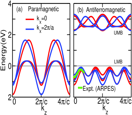
Figure 3: (color online) (a) Paramagnetic, and (b) AFM dispersions within the 2-band TB model as a function of $k_{z}$ at $k_{x}=0$ (red lines) and $k_{x}=2\pi/a$ (blue lines). Experimental ARPES datapoints are shown as green dots.takahashi

Table 1: TB parameters for 2-band model.

Parameter	This work		Ref. muller,
$\epsilon_{0}$	-0.0350(eV)		-0.0450(eV)
$t_{1}$	0.5650		0.5650
$t_{2}$	0.3800		0.3950
$t_{3}$	0.0400		0.0400
$t_{4}$	0.0520		0.0500
$t_{5}$	-0.1200		-0.1150
$t_{6}$	0.0700		0.0400
$t_{7}$	0.0750		0.0750
$t_{8}$	0.0057		0.0050
$t_{9}$	-0.0115		-0.0200

The trellis compound shows the presence of short-range spin order with a spin gap which is consistent with theoretical predictions dagotto . Due to the $180^{o}$ Cu₁-O₁-Cu₂ bonds, the spins are strongly coupled antiferromagnetically on the legs and the rungs of the ladders as indicated by green arrows in Fig. 1.alain However, the displacement of successive ladders with respect to each other frustrates the development of long range AFM order. One nevertheless expects the electronic system to experience significant AFM fluctuations, which are presumably sufficient to impose an underlying dispersion characteristic of the AFM order. In this spirit, we have approximated the correlation effects within a Hartree-Fock model of an itinerant AFM, as in the planar cupratesKusko . Taking the on-site energy to be $U$= 3.3 eV $\sim$ 6$t$, the magnetization was computed self-consistently to be $m$=0.43. The AFM Hamiltonian is given in the Appendix and the resulting dispersions are shown in Fig. 3(b). Comparison with the paramagnetic solution shows that a large gap of $\sim$2.3 eV opens up between the upper (UMB) and the lower magnetic bands (LMB). The theoretical LMBs display the characteristic backfolding near $k_{z}=\pi/2c$, which is in accord with the experimentally observed dispersion (green dots in Fig. 3(b) via ARPES takahashi , and is reminiscent of a similar effect in the insulating planar cuprates.

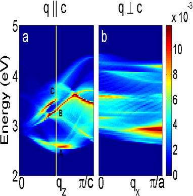
Figure 4: (color online) Color plots show computed RIXS spectra from SrCu₂O₃ for momentum transfer along (a): The ladder direction $q_{z}$ and (b): The direction $q_{x}$ perpendicular to the ladders. Theoretical spectra are not resolution broadened in order to highlight their intrinsic structure. Yellow vertical line marks the momentum transfer value where the detailed spectra, including features marked A-C, are considered in Fig. 5.

III RIXS Spectra

Our computations of the the K-edge RIXS cross section for the Cu $1s\rightarrow 4p$ core level excitation are based on the expression Mark ; nomura

$$\begin{array}[]{c}I(\textbf{q},\omega,\omega_{i})=(2\pi)^{3}N|W(\omega,\omega_{i})|^{2}\\ \times\sum_{j,j^{\prime},\textbf{k}}\chi^{"}_{jj^{\prime}}(\textbf{q},\textbf{k},\omega)|M{ij}(\textbf{k})|^{2}\par\end{array}$$ (1)

where

$$\begin{array}[]{c}\chi^{"}_{jj^{\prime}}(\textbf{q},\textbf{k},\omega)=\delta(\omega+E_{j}(\textbf{k})-E_{j^{\prime}}(\textbf{k}+\textbf{q}))\\ \times n_{j}(\textbf{k})[1-n_{j^{\prime}}(\textbf{q}+\textbf{k})],\end{array}$$ (2)

$n_{j}(k)$ is the electron occupation of the $j^{th}$ band and $E_{j}(k)$ is the corresponding energy dispersion obtained by self-consistently solving the two-band AFM Hamiltonian (see Appendix), and

$$\begin{array}[]{c}W(\omega_{f},\omega_{i})=|\gamma|\Sigma_{k_{1}}\frac{V_{d}}{D(\omega_{i},\textbf{k}_{1})D(\omega_{f},\textbf{k}_{2})}.\end{array}$$ (3)

Here, $D(\omega,\textbf{k})=\omega+\varepsilon_{1s}-\varepsilon_{4p}(k_{1})+i\Gamma_{1s}$, $\gamma$ is the matrix element for scattering from $1s$ to $4p$, and $V_{d}$ is the core-hole potential in $3d$ level. $\omega_{i}(\omega_{f})$ and $q_{i}(q_{f})$ denote the initial (final) energy and momentum, respectively, of the photon, and $\omega=\omega_{i}-\omega_{f}$ and $q=q_{i}-q_{f}$ give the energy and momentum transferred in the scattering process. Since Cu ${1s}$ is a core state, the associated energy band $\varepsilon_{1s}(k)$ is assumed dispersionless. The Cu ${4p}$ band dispersion $\varepsilon_{4p}(k)$ is modeled by a 2D-TB model with nearest neighbor hopping. $\Gamma_{1s}$ is the decay rate of core hole taken to be 0.8 eV. The matrix element $M_{i,j}$ associated with the interaction between the core hole and $3d$ levels around the Fermi energy is

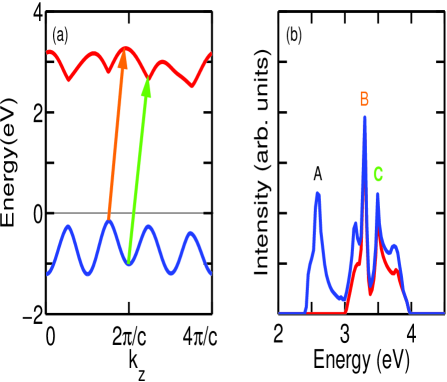
Figure 5: (color online) (a) Lowest and uppermost tight-binding AFM bands in SrCu₂O₃ at $k_{x}=0$. (b) Red line gives partial contribution to the RIXS spectrum at $q_{z}=\pi/{2c}$ (marked by yellow vertical line in Fig. 4(a)) from transitions between the two bands in (a). Blue line gives the corresponding total RIXS spectrum. Features A-C are discussed in the text.

$$\begin{array}[]{c}M_{ij}(\textbf{k})=\sum_{l,\sigma,\sigma^{\prime}}e^{i\textbf{q}\cdot\textbf{R}_{l}}\alpha_{l}X^{j}_{l\sigma}(\textbf{k})\Lambda^{j}_{\sigma,\sigma^{\prime}}(\omega,\textbf{q})X^{j^{\prime}}_{l\sigma^{\prime}}(\textbf{k}+\textbf{q}),\end{array}$$ (4)

in terms of the eigenvectors $X^{j}_{l\sigma}$ of the AFM Hamiltonian, where $\sigma$ denotes electron spin and $l$ an orbital index. $\alpha_{l}\equiv V_{l}/V_{d}$, where $V_{l}$ is the Coulomb interaction between a core hole and an electron on atom $l$ separated by a distance $R_{l}$. Here we approximate the vertex correction $\Lambda\rightarrow\delta_{\sigma,\sigma^{\prime}}$.

Fig. 4 shows RIXS spectra computed within the 2-band AFM model in the form of a color plot for momentum transfer along as well as perpendicular to the direction of the ladders. The d-band spectra have not been broadened in order to emphasize the presence of considerable intrinsic structure in the spectra, despite the large broadening $\Gamma$ associated with the short core hole lifetime. Insight into the nature of these spectra can be obtained by examining expressions 1-4 on which the computations are based. The enhancement factor $W(\omega_{i},\omega_{f})$ is found to vary relatively slowly with energy due to the large $4p$ bandwidth and the substantial damping of the core hole given by $\Gamma_{1s}$. Therefore, spectral shapes are controlled effectively by the term $\sum_{k}\delta(\omega+E_{j}(\textbf{k})-E_{j^{\prime}}(\textbf{k}+\textbf{q}))\times n_{j}(\textbf{k})[1-n_{j^{\prime}}(\textbf{q}+\textbf{k})]\mid X^{j}_{l\sigma}(\omega,\textbf{k})X^{j^{\prime}}_{l\sigma^{\prime}}(\omega,\textbf{k+q})\mid^{2}$. Note that this involves not only the joint density of states (JDOS) factor, $n_{j}(\textbf{k})[1-n_{j^{\prime}}(\textbf{q}+\textbf{k})]\delta(\omega+E_{j}(\textbf{k})-E_{j^{\prime}}(\textbf{k}+\textbf{q}))$, but also the partial electron occupancy of the filled band given by $\mid X^{j}_{l\sigma}(\omega,\textbf{k})\mid^{2}$ and the partial electron occupancy $\mid X^{j^{\prime}}_{l\sigma^{\prime}}(\omega,\textbf{k+q})\mid^{2}$ of the empty band. A large contribution thus results when JDOS connects band extrema, leading to resonant peaks in the RIXS cross-section.
Fig. 5 considers the spectrum at $q_{z}=\pi/{2c}$ in greater detail (i.e. corresponding to the vertical yellow line in Fig. 4(a)). The blue curve in Fig. 5(b) gives the total RIXS cross-section, which of course involves contributions from all allowed transitions from either of the two unfilled bands to one of the two empty bands in the AFM band structure of Fig. 3(b). The red curve in Fig. 5(b) gives the partial contribution to the spectrum from just the pair of bands shown in Fig. 5(a), i.e. the lowest occupied and the highest unoccupied band. In particular, peak C around 3.5 eV in Fig. 5(b) arises from transitions in (a) marked by the green arrow, while peak B has its origin in the transitions given by the orange arrow. [Note that the horizontal shift in the direction of the arrows in Fig. 5(a) is the momentum transfer vector, while the vertical displacement is the energy transferred in the scattering process.] Other spectral details can be analyzed in a similar manner and associated with specific transitions by examining the partial contributions from various pairs of bands. In particular, the resonant peak A around 2.5 eV in Fig. 5(b) results from transitions between the uppermost filled band and the lowest empty band in Fig. 3(a). Along these lines, the intense feature around 3 eV in the $q_{\perp}$ spectra of Fig.  4(b) is found to be associated with transitions between the uppermost filled band and the lowest empty band (as a function of $q_{\perp}$).

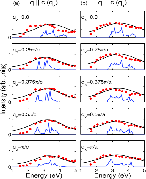
Figure 6: (color online) Comparison of unbroadened (blue curves) and broadened (black curves) RIXS spectra with the corresponding experimental data (red dots) taken from Ref. Hasan, . Left hand side panels are for $q_{\parallel}c$ at various $q_{z}$ values, while the right hand side panels are for $q_{\perp}c$ at various $q_{x}$ values as indicated. Spectra are normalized as shown.

Fig. 6 compares our theoretical spectra with the available experimental RIXS data of Ref. 12 on the ladder compound. Left hand side panels are for momentum transfer along the ladder direction (i.e. $q_{\parallel}c$) with $q_{z}$ varying from 0 to $\pi/c$, while the right hand side panels are for $q_{\perp}c$ with $q_{x}$ varying over the range 0-$\pi/a$. The unbroadened theoretical spectra (blue lines) require a substantial broadening for a meaningful comparison with the data (red dots). Accordingly, we have applied a combined Gaussian and Lorentzian broadening to the computed spectra to obtain the broadened theoretical spectra in Fig. 6 (black lines). The Gaussian broadening is taken as the nominal experimental resolution of 120 meVHasan . The residual broadening, which reflects presumably lifetime effects not accounted for in our computations, is modeled via a Lorentzian with half-width-at-half-maximum of $\Gamma_{d}$=1.1 eV for $q\parallel c$ and of $\Gamma_{d}$=1.4 eV for $q\perp c$foot1 ; ZHRIXS . Although Figs. 4-6 show that the RIXS spectra intrisically contain considerable information concerning the charge excitations and their momentum dependencies in the ladder compound, much of this structure is seen to be lost in the broadened spectra. Nevertheless, for both $q\parallel c$ as well as $q\perp c$, the experimental spectra are in reasonable accord with the broadened theory, some discrepancies in shape and fine structure in the experimental data notwithstanding. In particular, the spectra show a dispersion of $\sim 0.8eV$ along the ladders ($q_{z}$) and negligible dispersion perpendicular to the ladders ($q_{x}$). While we have compared our calculations to the data of Wray et al.Hasan , the undoped data of Ishii et al.Ishii show very similar broadening and dispersion, with a slightly larger gap.

IV Conclusions

We have presented a two-band model and the associated K-edge RIXS spectra for the ladder compound SrCu₂O₃ as a way of capturing the physics of the more complex ladder compound Sr₁₄Cu₂₄O₄₁. RIXS spectra are considered for momentum transfer along as well as perpendicular to the direction of the ladders. Our analysis indicates that the available ARPES and RIXS data are consistent within experimental resolution with the presence of strong antiferromagnetic correlations in the system, which are modeled in our study by introducing an ordered AFM state. Notably, our calculations do not require any significant renormalization of LDA-based band paramters in the ladder compound, and moreover, our value of the effective Hubbard $U$ is similar to that found in the insulating planar cupratesKusko .
Acknowledgements This work is supported by the U.S.D.O.E contracts DE-FG02-07ER46352, AC03-76SF00098 and benefited from the allocation of supercomputer time at NERSC and Northeastern University’s Advanced Scientific Computation Center (ASCC). MZH is supported by DOE/DE-FG02-05ER46200.

Appendix: AFM and Paramagnetic Hamiltonians and Dispersions

The AFM Hamiltonian for the two band model can be written as

$$\begin{array}[]{c}H=\sum_{j}\varepsilon_{0}d_{j}^{+}d_{j}+\sum_{<i,j>}t_{ij}(d_{j}^{+}d_{i}+d_{j}d_{i}^{+})+\\ \sum_{j}Un_{d_{j}\uparrow}n_{d_{j}\downarrow}\end{array}$$ (5)

where $n_{d_{j}}=d_{j}^{+}d_{j}$, $\varepsilon_{0}$ is the on site energy, $t_{ij}$’s are the hopping parameters (see Fig. 1), and $U$ is Hubbard U. The AFM ordering of spins is shown in Fig. 1 by green arrows. The Hartree-Fock decomposition of the Hubbard term in the Hamiltonian is given by

$$\begin{array}[]{c}n_{d_{j}\uparrow}n_{d_{j}\downarrow}\rightarrow\\ n_{d_{j}\uparrow}<n_{d_{j}\downarrow}>+<n_{d_{j}\uparrow}>n_{d_{j}\downarrow}-\\ <n_{d_{j}\uparrow}><n_{d_{j}\downarrow}>\\ U_{m}=\frac{U}{2}(<n_{d_{j}\uparrow}>-<n_{d_{j}\downarrow}>)=Um\\ <n>=<n_{d_{j}\uparrow}>+<n_{d_{j}\downarrow}>\end{array}$$ (6)

We can now rewrite the AFM Hamiltonian as

$${\mathcal{H}}_{11} = {\mathcal{H}}_{44}=\triangle+U_{m},~{}~{}~{}~{}{\mathcal{H}}_{22}={\mathcal{H}}_{33}=\triangle-U_{m}$$ (7)

$$\newline {\mathcal{H}}_{12} = -t_{2}-t_{3}\exp(ik_{x}/2)-t_{6}\exp(3ik_{z}/2)-2t_{8}\cos(2k_{z}),$$

$$\newline {\mathcal{H}}_{13} = -2t_{1}\cos(k_{z})-2t_{4}\cos((k_{z}-k_{x})/2)-2t_{9}\cos((3k_{z}-k_{x})/2),$$

$$\newline {\mathcal{H}}_{14} = -2t_{5}\cos(k_{z})-t_{3}\exp(-i(k_{z}-k_{x})/2)-t_{6}\exp(-i(3k_{z}+k_{x})/2),$$

$$\newline {\mathcal{H}}_{23} = -2t_{5}\cos(k_{z})-t_{3}\exp(i(k_{z}-k_{x})/2)-t_{6}\exp(i(3k_{z}-k_{x})/2),$$

$$\newline {\mathcal{H}}_{24} = -t_{1}\cos(k_{z})-2t_{4}\cos((k_{z}+k_{x})/2)-2t_{9}\cos((3k_{z}+k_{x})/2)),$$

$$\newline {\mathcal{H}}_{34} = {\mathcal{H}}_{12},$$

where

$$\triangle = \varepsilon_{\circ}-2t_{7}\cos(2k_{z})-2t_{4}\cos((k_{z}+k_{x})/2)-2t_{9}\cos((3k_{z}-k_{x})/2)).$$

For the the paramagnetic case $U_{m}$ is equal to zero and the $4\times 4$ AFM Hamiltonian is reduced to a $2\times 2$ form with matrix elements

$${H}_{11}={H}_{22} = \epsilon_{0}-2t_{1}\cos(k_{z})-2t_{7}\cos(2k_{z})-4t_{4}\cos(k_{x}/2)\cos(k_{z}/2)-4t_{9}\cos(k_{x}/2)\cos(3k_{z}/2),$$ (8)

$$\newline {H}_{12} = -t_{2}-2t_{5}\cos(k_{z})-2t_{8}\cos(2k_{z})-2t_{3}\exp(ik_{x}/2)\cos(k_{z}/2)-2t_{6}\exp(ik_{x}/2)\cos(3k_{z}/2),$$

The resulting dispersion ismuller

$$\varepsilon_{\pm}(\textbf{k})=\epsilon_{0}+\epsilon_{\|}(k_{z})\cos(k_{x}/2)+(\epsilon_{\bot,1}(k_{z})\cos(k+x/2)\pm(\epsilon_{\bot,3}(k_{z})^{2}+\epsilon_{\bot,4}(k_{z})^{2}+2\epsilon_{\bot,3}(k_{z})\epsilon_{\bot,3}(k_{z})\cos(k_{x}/2))^{1/2}$$ (9)

where

$$\epsilon_{\|}(k_{z}) = -2t_{1}\cos(k_{z})-2t_{7}\cos(2k_{z}),$$ (10)

$$\newline \epsilon_{\bot,1}(k_{z}) = -4t_{4}\cos(k_{z}/2)-4t_{9}\cos(3k_{z}/2),$$

$$\newline \epsilon_{\bot,3}(k_{z}) = t_{2}+2t_{5}\cos(k_{z})+2t_{8}\cos(2k_{z}),$$

$$\newline \epsilon_{\bot,4}(k_{z}) = 2t_{3}\cos(k_{z}/2)+2t_{6}\cos(3k_{z}/2),$$

References

- (1) A. Kotani and S. Shin, Rev. Mod. Phys. 73, 203 (2001).
- (2) T. Nagata, M. Uehara, J. Goto, J. Akimitsu, N. Motoyama, H. Eisaki, S. Uchida, H. Takahashi, T. Nakanishi, and N. Môri, Phys. Rev. Lett. 81, 1090 (1998).
- (3) P. Abbamonte, G. Blumberg, A. Rusydi, A. Gozar, P. G. Evans, T. Siegrist, L. Venema, H. Eisaki, E. D. Isaacs, G. A. Sawatzky Nature 431, 1078 (2004).
- (4) L. Wray, D. Qian, D. Hsieh, Y. Xia, H. Eisaki, and M. Z. Hasan Phys. Rev. B 76, 100507(R) (2007).
- (5) K. Ishii, K. Tsutsui, T. Tohyama, T. Inami, J. Mizuki, Y. Murakami, Y. Endoh, S. Maekawa, K. Kudo, Y. Koike, and K. Kumagai, Phys. Rev. B 76, 045124 (2007).
- (6) M. Arai, and H. Tsunetsugu, Phys. Rev. B 56, R4305 (1997).
- (7) T.F.A. Mller , V. Anisimov, T. M. Rice, I. Dasgupta, and T. Saha-Dasgupta, Phys. Rev. B 57, R12655 (1998).
- (8) D.C. Johnston, M. Troyer, S. Mayhara, D. Lidsky, K. Ueda, M. Azuma, Z. Hiroi, M. Takano, M. Isobe, Y. Ueda, M. A. Korotin, V. I. Ansimov, A. V. Mahajan, and L. L. Miller, cond-mat/0001147.
- (9) P. Blaha, K. Schwarz, G.K.H. Madsen, D. Kvasnicka, and J. Luitz, WIEN2k, An Augmented Plane Wave + Local Orbitals Program for Calculating Crystal Properties (Technische Universitat, Vienna, 2001).
- (10) A. Bansil, S. Kaprzyk, P. E. Mijnarends, and J. Tobola, Phys. Rev. B 60, 13396 (1999).
- (11) A. Bansil, M. Lindroos, S. Sahrakorpi, and R.S. Markiewicz, Phys. Rev. B71, 012503 (2005).
- (12) E. Dagotto, and T.M. Rice, Science 271, 618 (1996).
- (13) A. Gellé, and M-B. Lepetit, Phys. Rev. Lett 92, 236402 (2004).
- (14) C. Kusko, R. S. Markiewicz. M. Lindroos, and A. Bansil, Phys. Rev. B 66, 104513(R) (2002).
- (15) T. Takahashi, T. Yokoya, A. Ashihara, O. Akaki, H. Fujisawa, A. Chainani, M. Uehara, T. Nagata, J. Akimitsu, and H. Tsunetsugu, Phys. Rev. B 56, 7870 (1997).
- (16) R.S. Markiewicz, and A. Bansil, Phys. Rev. Lett. 96, 107005 (2006).
- (17) Takuji Nomura, Jun-ichi Igarashi, J. Phys. Soc. Jpn. 73, 3171-3176 (2004).
- (18) Interestingly, these values of are substantially larger than those found previously in analyzing RIXS data from an electron-doped planar cuprate ZHRIXS .
- (19) Y.W. Li, D. Qian, L. Wray, D. Hsieh, Y. Kaga, T. Sasagawa, H. Takagi, R.S. Markiewicz, A. Bansil, H. Eisaki, S. Uchida, M.Z. Hasan, cond-mat/0704.3111v1.