Drude weight in systems with open boundary conditions

Abstract

For finite systems, the real part of the conductivity is usually decomposed as the sum of a zero frequency delta peak and a finite frequency regular part. In studies with periodic boundary conditions, the Drude weight, i.e., the weight of the zero frequency delta peak, is found to be nonzero for integrable systems, even at very high temperatures, whereas it vanishes for generic (nonintegrable) systems. Paradoxically, for systems with open boundary conditions, it can be shown that the coefficient of the zero frequency delta peak is identically zero for any finite system, regardless of its integrability. In order for the Drude weight to be a thermodynamically meaningful quantity, both kinds of boundary conditions should produce the same answer in the thermodynamic limit. We shed light on these issues by using analytical and numerical methods.

Transport properties define materials as superconductors, metals, or insulators.kohn64 ; shastry90 ; scalapino92 In one dimension, transport can help differentiate integrable from nonintegrable systems. Integrable systems, in general, display an infinite conductivity at all temperatures,castella95 an effect that has been related to the strong influence of conservation laws, while at high temperatures, generic (nonintegrable) systems are expected to exhibit a finite resistivity caused by umklapp scattering and inelastic collisions.

Let us consider a finite system of length $L$ (in units of the lattice constant); the real part of the conductivity can be written ascastella95 ; shastry90 ; shastry06

$$\textrm{Re}\left[\sigma_{L}(\omega)\right] = \pi D_{L}\delta(\hbar\omega)+\frac{\pi}{L}\left(\frac{1-e^{-\beta\hbar\omega}}{\omega}\right)$$ (1)

$$\times\sum_{\epsilon_{n}\neq\epsilon_{m}}p_{n}|J_{nm}|^{2}\delta(\epsilon_{m}-\epsilon_{n}-\hbar\omega),$$

where

$$D_{L}=\frac{1}{L}\left[\langle\hat{\Gamma}\rangle-\hbar\sum_{\epsilon_{n}\neq\epsilon_{m}}\frac{p_{n}-p_{m}}{\epsilon_{m}-\epsilon_{n}}|J_{nm}|^{2}\right],$$ (2)

is the Drude weight (or charge stiffness), the stress tensor operator $\hat{\Gamma}=-q_{e}\lim_{k\rightarrow 0}\frac{1}{k}[\hat{J}(k),\hat{n}(-k)]$, $\hat{J}$ is the current operator, $J_{nm}=\langle n|\hat{J}|m\rangle$ are its matrix elements, $\hat{n}(k)$ is the Fourier transform of the local density operator $\hat{n}_{j}$, $q_{e}$ the charge, and $\Gamma=\langle\hat{\Gamma}\rangle/\hbar L$. The Boltzmann weight of a state $|m\rangle$ is denoted by $p_{m}=e^{-\beta\epsilon_{m}}/Z$, with $\epsilon_{m}$ being its energy, $\beta=1/k_{B}T$, and $Z$ the partition function.

In one dimension, and finite temperatures, the Drude weight can also be computed as,castella95 ; shastry06 (assuming that there is no true superconductivity)

$$D^{*}_{L}=\frac{\beta\hbar}{L}\sum_{\epsilon_{n}=\epsilon_{m}}p_{n}|J_{nm}|^{2}.$$ (3)

Equation (1) is true for all boundary conditions. In the thermodynamic limit (TL), it leads to the decomposition $\textrm{Re}\left[\sigma_{\infty}(\omega)\right]=\pi D_{\infty}\delta(\hbar\omega)+\sigma_{reg}(\omega)$, where the infinite volume object $D_{\infty}=\lim_{L\rightarrow\infty}D_{L}=\lim_{L\rightarrow\infty}D^{*}_{L}$, and $\sigma_{reg}$ is the “regular” part of the conductivity. In systems with periodic boundary conditions (pbc’s), $D_{L}$ and $D^{*}_{L}$ are found to be nonzero in integrable systems at all temperatures, i.e., they display an infinite conductivity, whereas $D_{L}$ and $D^{*}_{L}$ are expected to exponentially vanish with the system size for nonintegrable systems.castella95 ; fabian03

A very different situation arises when one studies systems with open boundary conditions (obc’s). There, one can legitimately defineshastry06 the position operator $\hat{X}=\sum_{j}j\,\hat{n}_{j}$, which satisfies the following commutation relations: $\hat{J}=i[\hat{X},\hat{H}]$, where $\hat{H}$ is the Hamiltonian of the system and $\hat{\Gamma}=-i[\hat{X},\hat{J}]$. Since $J_{nm}=i(\epsilon_{m}-\epsilon_{n})\langle n|\hat{X}|m\rangle$, one can see that $D^{*}_{L}$ (3) is identically zero, and that the first and second terms in the right hand side of Eq. (2) cancel each other, so that $D_{L}$ is also identically zero. The vanishing of $D_{L}$ and $D^{*}_{L}$ for systems with obc’s is true regardless of their integrability.

Considering the results above, one could question whether the Drude weight is a meaningful thermodynamic quantity, i.e., whether one would obtain the same result, measuring it in (quasi-) one-dimensional (1D) experiments involving closed rings or open chains. This is a valid concern since $D_{\infty}$ is not a usual bulk thermodynamic quantity. (For the latter, the equivalence of boundary conditions in the TL is obvious.) In an expansion of the energy of the system in powers of $L$, $D_{\infty}$ at $T=0$ is proportional to a term that scales like $1/L$.kohn64 ; shastry90 Our goal in this work is to shed light on this puzzle.

We consider 1D systems of spinless fermions,

$$\hat{H} = -t\sum_{j}\hat{c}^{\dagger}_{j}\hat{c}_{j+1}+\textrm{h.c.}+V\sum_{j}\hat{n}_{j}\hat{n}_{j+1}$$ (4)

$$-t^{\prime}\sum_{j}\hat{c}^{\dagger}_{j}\hat{c}_{j+2}+\textrm{h.c.}+V^{\prime}\sum_{j}\hat{n}_{j}\hat{n}_{j+2}$$

with nearest ($t$) and next-nearest ($t^{\prime}$) neighbor hopping, interacting with nearest ($V$) and next-nearest ($V^{\prime}$) neighbor repulsive potentials. The sum over $j$ is appropriately defined for pbc’s and obc’s. $c^{\dagger}_{j}$ ($c_{j}$) are the creation (annihilation) operators for spinless fermions at a given site $j$, and $\hat{n}_{j}=c^{\dagger}_{j}c_{j}$ are the corresponding density operators. This model is known to be integrable for $t^{\prime}=V^{\prime}=0$. (It can be mapped onto the XXZ spin 1/2 chain.) To understand the effects of obc’s in more generic nonintegrable systems, we study systems with finite values of $t^{\prime}$ and $V^{\prime}$.

The current and stress tensor operators for this model can be written as

$$\hat{J} = \frac{iq_{e}t}{\hbar}\sum_{j}\hat{c}^{\dagger}_{j}\hat{c}_{j+1}+\textrm{H.c.}+\frac{2iq_{e}t^{\prime}}{\hbar}\sum_{j}\hat{c}^{\dagger}_{j}\hat{c}_{j+2}+\textrm{H.c.},$$

$$\hat{\Gamma} = \frac{q^{2}_{e}t}{\hbar}\sum_{j}\hat{c}^{\dagger}_{j}\hat{c}_{j+1}+\textrm{H.c.}+\frac{2q^{2}_{e}t^{\prime}}{\hbar}\sum_{j}\hat{c}^{\dagger}_{j}\hat{c}_{j+2}+\textrm{H.c.}.$$

As a starting point for our analysis, let us consider the case of noninteracting fermions. With pbc’s, the single-particle eigenstates of the Hamiltonian are plane waves $|m\rangle=1/\sqrt{L}\sum_{j}e^{ik_{m}j}\hat{c}^{\dagger}_{j}|0\rangle$ with energy $\epsilon_{m}=-2t\,\cos(k_{m})$, where $k_{m}=2\pi m/L$ and $m=-L/2+1,\ldots,L/2$. In this case, $|J_{nm}|^{2}=[2q_{e}t\,\sin(k_{m})]^{2}\delta_{m,n}$, i.e., the matrix elements of $\hat{J}$ are fully diagonal, and $D_{L}=\langle\hat{\Gamma}\rangle/\hbar L=q^{2}_{e}\langle\hat{H}\rangle/\hbar L$. At finite temperatures, and for sufficiently large system sizes, $D_{L}^{*}=D_{L}$.

For obc’s, on the other hand, standing waves being the noninteracting eigenstates, have the form $|m\rangle=\sqrt{2/(L+1)}\sum_{j}\sin(k_{m}j)\hat{c}^{\dagger}_{j}|0\rangle$ with energy $\epsilon_{m}=-2t\,\cos(k_{m})$, where $k_{m}=\pi m/(L+1)$ and $m=1,\ldots,L$. The matrix elements of the current operator are then

$$|J_{nm}|^{2}=\frac{8q^{2}_{e}t^{2}}{(L+1)^{2}}\left[1-(-1)^{(m-n)}\right]\frac{\sin^{2}(k_{m})\sin^{2}(k_{n})}{\left[\cos(k_{m})-\cos(k_{n})\right]^{2}},$$

and vanish whenever $(m-n)$ is an even number, i.e., only eigenstates with a different parity produce nonvanishing values of $J_{nm}$. This expression shows that the matrix elements of $\hat{J}$ have a very interesting property: although $|J_{nm}|$ vanish for $m=n$, they attain their largest values for the smallest (odd) differences between $m$ and $n$. For very large systems, the factor $1/L^{2}$ produces vanishing values of $J_{nm}$ unless $n\sim m$. Rewriting $k_{n}=k_{m}\pm\pi l/(L+1)$, $l=1,3,\ldots$ one can see that $\textrm{Re}\left[\sigma(\omega)\right]$ is a sum of delta functions $\delta[\omega\pm 2\pi t\,\sin(k_{m})l/(L+1)]$ whose weight decreases as $\sim 1/l^{2}$.

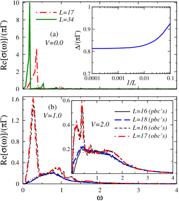
Figure 1: (color online). Regular part of $\textrm{Re}\left[\sigma(\omega)\right]$ for integrable systems ($t^{\prime}=V^{\prime}=0$) in (a) the noninteracting case ($V=0$), (b) $V=1.0$, and [inset in (b)] the isotropic (Heisenberg) point $V=2.0$. All of these results were obtained at a very high temperature $\beta=0.001$ (infinite in the noninteracting case) and half-filling. The inset in (a) shows how $\Delta$ (see text) behaves as one approaches the TL. The values of $V$, $\beta$, and $\omega$ are given in units of $t$.

In Fig. 1(a), we show $\textrm{Re}\left[\sigma(\omega)\right]$ (binned to obtain a smooth curve) for noninteracting particles in two systems with obc’s and different sizes. This figure shows that (i) broadened delta functions collapse to larger peaks (whose width reduces as the system size increases) situated at $\omega\sim 2\pi l/L$ with $l=1,3,\ldots$, and (ii) these peaks move toward smaller frequencies as $L$ increases. From the previous analysis, one can conclude that although for finite open systems $D_{L}$ and $D^{*}_{L}$ are always zero, for $L\rightarrow\infty$, a delta peak develops at $\omega=0$, but this time generated by the collapse of delta peaks that come from the so-called regular part of the conductivity. In addition, from the sum rule $\int_{-\infty}^{\infty}\textrm{Re}\left[\sigma(\omega)\right]d\omega={\pi}\langle\hat{\Gamma}\rangle/\hbar L$,shastry06 one obtains that the weight of such $\omega=0$ peak is $\pi D_{\infty}=\lim_{L\rightarrow\infty}\pi\langle\hat{\Gamma}\rangle/\hbar L=\lim_{L\rightarrow\infty}\pi q^{2}_{e}\langle\hat{H}\rangle/\hbar L$, which is identical to $\pi D_{\infty}$ as obtained from periodic systems since the energy is identical in both cases.

At this point, one may wonder about the behavior of the finite frequency ($\omega\sim\pm 2\pi l/L$, $l=1,3,\ldots$) peaks as $L$ is increased. It may happen that as $L\rightarrow\infty$, (i) all the weight is concentrated in the lowest $\omega=\pm 1/L$ peaks, and the others disappear, or (ii) the weight is distributed among several peaks with different values of $\omega$. To answer this question, we have studied the summed weight of the peaks at $\omega\sim\pm 2\pi/L$ as a function of increasing system size, a quantity we call $\Delta$. Results are shown in the inset in Fig. 1(a). They confirm the scenario (ii) above since, as $L\rightarrow\infty$, $\Delta$ saturates at around 80% of $\pi\Gamma$. Hence, the other peaks with $l>1$ remain finite, and they are needed to account for the exact Drude weight in the TL.

Moving away from the noninteracting case, but keeping the system integrable, we cannot make the corresponding analytical treatment, so we turn to a full exact diagonalization of finite chains. We perform calculations in the grand-canonical ensemble, and all results presented in what follows are obtained at half-filling ($n=0.5$).

For generic integrable systems with pbc’s, the matrix elements of $\hat{J}$ are not diagonal anymore like in the noninteracting case. This means that weight moves away from the Drude peak and the regular part of $\textrm{Re}\left[\sigma(\omega)\right]$ becomes finite. This can be seen in Fig. 1(b) and its inset, where we have plotted $\textrm{Re}\left[\sigma(\omega)\right]$ for two integrable systems with different values of $V$. The scaling of the Drude weight with system size, together with a “simple minded” linear extrapolation to the TL, are shown in Fig. 2(a). As seen there, for both $V=1.0$ and $V=2.0$, we obtain a finite value of $D_{\infty}$.shastry90 ; castella95 ; fabian03 ; mukerjee07

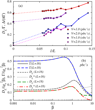
Figure 2: (color online). (a) Scaling of the Drude weight (pbc’s) and $\Delta$ (obc’s) with the system size, for $V=1.0$ and $2.0$ and $\beta=0.001$. (b) The Drude weight, computed as $D_{L}$ and $D^{*}_{L}$, and $\Gamma$ as a function of $\beta$ for the isotropic case ($V=2.0$).

The results presented so far were obtained at a very high temperature ($\beta=0.001$), where finite size effects are the smallest, but transport properties are still nontrivial. In Fig. 2(b), one can see that for $T>10$, the actual value of $T$ is not essential since quantities such as $D_{L}T$, $D^{*}_{L}T$, and $\Gamma T$ become almost independent of $T$. Figure 2(b) also shows that, for the considered temperatures and system sizes, $\Gamma$ is independent of the system size, while $D_{L}$ and $D^{*}_{L}$ still exhibit finite size effects. It is important to notice that albeit $D_{L}$ and $D^{*}_{L}$ are identical for any given system size at high temperatures, finite size effects build differences between these two ways of computing the Drude weight at lower temperatures.fabian03

After reviewing the pbc case, we can now analyze the effects of obc’s on more generic integrable systems. In Fig. 1(b) and its inset, we have plotted $\textrm{Re}\left[\sigma(\omega)\right]$ for chains with obc’s, and two different values of $V$, together with the results for pbc’s. One can clearly see there that large peaks develop in the obc data over the pbc results, and that these peaks move toward lower frequencies as $L$ is increased.kuhner00 Actually, for $V=1.0$, one can see that the two largest obc peaks are located at $\omega\sim 2\pi l/L$, $l=1$ and 3, similar to the noninteracting case. These results strongly suggest that in the TL, the finite frequency peaks for obc’s will collapse into a single $\omega=0$ Drude peak like the one obtained for pbc’s.

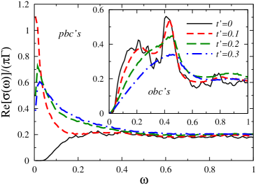
Figure 3: (color online). Regular part of $\textrm{Re}\left[\sigma(\omega)\right]$ for nonintegrable systems with pbc’s ($L=17$) and (inset) obc’s ($L=16$) as one moves away from the isotropic integrable point by increasing the value of $t^{\prime}$. In all cases, $V=2.0$ and $\beta=0.001$.

In Fig. 2(a), we show how $\Delta$ behaves with increasing system size for $V=1.0$ and $V=2.0$. [$\Delta$ is computed in this case as two times the area over the dotted lines in Fig. 1(b).] In both cases, the behavior of $\Delta$ is consistent with extrapolated $\omega=0$ peaks with a finite weight in the TL. Like for the noninteracting case, extrapolating $\Delta$ to $L\rightarrow\infty$ does not reproduce the value of $D_{\infty}$ obtained for systems with pbc’s. This, we infer, is due to the weight distributed over peaks with higher frequencies, which, following the noninteracting case, should all collapse to $\omega=0$ as $L\rightarrow\infty$. The extrapolations in Fig. 2(a) show that the relative weight of peaks with higher $\omega$ in chains with obc’s increases as one departs from the noninteracting case.

Having shed light on integrable systems, we now turn to the nonintegrable case. As mentioned before, in systems with pbc’s, breaking integrability is expected to produce an exponentially (with the system size) vanishing Drude weight. We first consider (Fig. 3) the case in which in Eq. (4) integrability is broken by $t^{\prime}$, which also breaks the particle-hole symmetry of the integrable model. In Fig. 3, one can see that, even for small finite systems, introducing $t^{\prime}$ has dramatic effects in $\textrm{Re}\left[\sigma(\omega)\right]$. A peak develops at low frequencies. Given the sum rule for $\textrm{Re}\left[\sigma(\omega)\right]$, such a peak can be related to the disappearance of the Drude peak and the transfer of its weight to finite frequencies. Hence, the system acquires a finite dc conductivity, which decreases with increasing $t^{\prime}$ (Fig. 3).

For small finite systems with obc’s, on the other hand, nothing dramatic should happen when a small $t^{\prime}$ is introduced. This is because in the integrable case, there is no zero frequency delta peak, but, instead, finite frequency peaks that are already present in the regular part of $\textrm{Re}\left[\sigma(\omega)\right]$. As seen in the inset in Fig. 3, adding $t^{\prime}$ to integrable chains with obc’s only reduces the height of the lowest frequency peak in $\textrm{Re}\left[\sigma(\omega)\right]$ and, with increasing $t^{\prime}$, its weight moves toward higher frequencies.

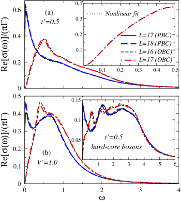
Figure 4: (color online). Regular part of $\textrm{Re}\left[\sigma(\omega)\right]$ for nonintegrable chains with different system sizes. (a) $t$-$t^{\prime}$-$V$ model with $t^{\prime}=0.5$, (b) $t$-$V$-$V^{\prime}$ model with $V^{\prime}=1.0$, and [inset in (b)] $t$-$t^{\prime}$-$V$ model for a system of hard-core bosons with $t^{\prime}=0.5$. The inset in (a) shows the low-frequency part of $\textrm{Re}\left[\sigma(\omega)\right]$ for the fermionic $t$-$t^{\prime}$-$V$ model together with a nonlinear fit (see text). In all cases, $V=2.0$, $\beta=0.001$, and $t^{\prime}$, $V$, $V^{\prime}$, $\beta$, and $\omega$ are given in units of $t$.

An apparent difference between $\textrm{Re}\left[\sigma(\omega)\right]$ in systems with pbc’s and systems with obc’s (Fig. 3) is that, while the former exhibit a finite dc conductivity, the latter exhibit a vanishing one. The vanishing of the dc conductivity for finite systems with obc’s is understandable by using an analogy with pbc’s with a small but finite momentum $q$. For $q\neq 0$, we know from the conservation law [$\omega\,\hat{n}(q,\omega)\simeq q\,\hat{J}(q,\omega)$] that the current must vanish in the dc limit.mukerjee07 One expects, in this case, to see diffusion, i.e., $\sigma(q,\omega)=\sigma(0,\omega)/[1-iDq^{2}/\omega]$ with $q\sim\pi/L$ for obc’s. This means that at very low frequencies for obc’s, $\textrm{Re}\left[\sigma(\omega)\right]\sim\omega^{2}$. As shown in the inset in Fig. 4(a), our data are crudely consistent with that. There, we also show the result of a nonlinear fit to $\textrm{Re}\left[\sigma(\omega)\right]=\sum_{a=1,6}C_{a}\omega^{a}$, where we find that $C_{1}\simeq 0$.

From the previous analysis, one expects the region of $\omega$’s over which $\textrm{Re}\left[\sigma(\omega)\right]\rightarrow 0$ to reduce with increasing $L$ and, eventually, in the TL, to recover the $k=0$ result obtained for pbc’s. In the main panel of Fig. 4(a), we depict results for pbc’s and obc’s in systems with two different sizes. There, one can see that, indeed, for obc’s, the low-frequency region with decreasing conductivity moves to lower frequencies with increasing system size. In the TL, the usual belief is that long time tails in the autocorrelation of the current will ultimately take over, asymptotically leading to $\textrm{Re}\left[\sigma(\omega)\right]\sim A-B\sqrt{|\omega|}$.mukerjee06

We should stress that our conclusions above are valid for generic nonintegrable systems, i.e., they are not limited to the $t$-$t^{\prime}$-$V$ model presented in Figs. 3 and 4(a). For example, in Fig. 4(b) we show that similar results are obtained when $t^{\prime}$=0 but $V^{\prime}$$\neq$$0$ ($t$-$V$-$V^{\prime}$ model, main panel), and $V^{\prime}$=0, $t^{\prime}$$\neq$$0$ ($t$-$t^{\prime}$-$V$ model), but for a system of hard-core bosons (inset). The last two models preserve the particle-hole symmetry present in the integrable case, so our conclusions are also independent of its presence or absence in nonintegrable systems.

In summary, we have argued that even though the real part of the conductivity in finite systems with obc’s is qualitatively different from that of systems with pbc’s, they both have a common thermodynamic limit. For integrable systems, this means that there is an infinite dc conductivity, characterized by a finite Drude weight. On the other hand, for nonintegrable systems, the dc conductivity is finite and, in our 1D systems, it decreases as one moves away from the integrable point.

- (1)
- (2) W. Kohn, Phys. Rev. 133, A171 (1964).
- (3) B. S. Shastry and B. Sutherland, Phys. Rev. Lett. 65, 243 (1990).
- (4) D. J. Scalapino, S. R. White, and S. C. Zhang, Phys. Rev. Lett. 68, 2830 (1992); Phys. Rev. B 47, 7995 (1993).
- (5) H. Castella, X. Zotos, and P. Prelovšek, Phys. Rev. Lett. 74, 972 (1995); X. Zotos, F. Naef, and P. Prelovšek, Phys. Rev. B 55, 11029 (1997), and references therein.
- (6) B. S. Shastry, Phys. Rev. B 73, 085117 (2006).
- (7) F. Heidrich-Meisner et al., Phys. Rev. B 66, 140406(R) (2002); 68, 134436 (2003).
- (8) S. Mukerjee and B. S. Shastry, arXiv:0705.3791.
- (9) T. D. Kühner, S. R. White, and H. Monien, Phys. Rev. B 61, 12474 (2000).
- (10) S. Mukerjee, V. Oganesyan, and D. Huse, Phys. Rev. B 73, 035113 (2006); T. R. Kirkpatrick, D. Belitz, and J. V. Sengers, J. Stat. Phys. 109, 373 (2002).