Capacity of The Discrete-Time Non-Coherent Memoryless Rayleigh Fading Channels at Low SNR

Abstract

The capacity of a discrete-time memoryless channel, in which successive symbols fade independently, and where the channel state information (CSI) is neither available at the transmitter nor at the receiver, is considered at low SNR. We derive a closed form expression of the optimal capacity-achieving input distribution at low signal-to-noise ratio (SNR) and give the exact capacity of a non-coherent channel at low SNR. The derived relations allow to better understanding the capacity of non-coherent channels at low SNR and bring an analytical answer to the peculiar behavior of the optimal input distribution observed in a previous work by Abou Faycal, Trott and Shamai. Then, we compute the non-coherence penalty and give a more precise characterization of the sub-linear term in SNR. Finally, in order to better understand how the optimal input varies with SNR, upper and lower bounds on the capacity-achieving input are given.

I INTRODUCTION

In wireless communication, the channel estimation at the receiver is not often possible due, for instance, to the high mobility of the sender or the receiver or both. Therefore, achieving reliable communication over fading channels where the channel state information (CSI) is available neither at the transmitter nor at the receiver, is of a particular interest. Establishing the performance limits, in terms of channel capacity, error probability, etc.., in such a non-coherent scenario has recently motivated extensive works (see for example [1], [2]). When CSI is available at the receiver, the channel capacity, commonly known as the coherent capacity has been studied by Ericson [3] for a Single Input Single Output (SISO) channel and recently by many other authors for a Multiple Input Multiple Output (MIMO) channel [4] [5]. Conversely, when CSI is not available at both ends, computing the channel capacity, known as the non-coherent capacity, as well as computing the optimal input distribution achieving this capacity, for both SISO and MIMO channels, is a rather tedious task [6] [7]. The main difficulty in computing the non-coherent capacity relies on the fact that the capacity-achieving input distribution is discrete with a finite number of mass points, where one of them is located at the origin. The number of these mass points increases with the signal-to-noise ratio (SNR). Since no bound on the number of mass points with respect to SNR is actually available, it is very difficult to find closed form expressions for both the achievable capacity and the optimal input distribution for all SNR values. Fortunately, numerical computation of the capacity and the optimal input distribution has been made possible using the Khun-Tucker condition which is a necessary and sufficient condition for optimality, for of a SISO channel [6] and for a MIMO channel [7].

Earlier in 1999, using a block fading channel, Marzetta and Hochwald have obtained the structure of the optimal input, with explicit calculations for the special case of a SISO channel at high SNR values or with a large coherence time [8]. The non-coherent capacity was also computed as a function of the number of transmit and receive antennas as well as the coherence time at high SNR in [9]. At a low SNR regime, it was also shown in [9] that to a first order of magnitude of the SNR, there is no capacity penalty for not knowing the channel at the receiver which is not the case at the high SNR regime. It has been well established previously that at low SNR, just like in an additive white Gaussian noise (AWGN) channel, the capacity of a fading channel varies linearly with the SNR regardless of whether or not the CSI is available at the receiver [10], [11]. Recently, this power efficiency at a low SNR regime or equivalently at a large channel bandwidth has motivated work towards a better understanding of the non-coherent capacity at a low SNR regime [1], [13], [14] for both SISO and MIMO channels using several fading models.

In this paper, we analyze the capacity of a discrete time non-coherent memoryless Rayleigh fading SISO channel at low SNR. The main contributions of this paper are:

1. Derivation of an analytical closed form of the channel mutual information at low SNR, which may also be considered as a lower bound on the channel mutual information for an arbitrary SNR value.

2. Derivation of a fundamental relation between the capacity-achieving input distribution and the SNR value, from which an exact capacity expression is deduced at low SNR.

3. Derivation of novel upper and lower bounds on the non-zero mass point location of the optimal input, which allow to deduce lower and upper bounds respectively on the non-coherent capacity at low SNR.

The paper is organized as follows. Section II presents the system model. In section III, we derive a closed form expression of the channel mutual information at low SNR which is also a lower bound on the channel mutual information at all SNR values. The optimal input distribution as well as the non-coherent capacity are presented in Section IV. Numerical results are reported in Section V and Section VI concludes the paper.

II CHANNEL MODEL

We consider a discrete-time memoryless Rayleigh-fading channel given by:

$$r(l)=h(l)s(l)+w(l),\hskip 28.45274ptl=1,2,3,...$$ (1)

where $l$ is the discrete-time index, $s(l)$ is the channel input, $r(l)$ is the channel output, $h(l)$ is the fading coefficient and $w(l)$ is an additive noise. More specifically, $h(l)$ and $w(l)$ are independent complex circular Gaussian random variables with mean zero and variances $\sigma_{h}^{2}$ and $\sigma_{w}^{2}$, respectively. The input $s(l)$ is subject to an average power constraint, that is $E[|s(l)|^{2}]\leq P$, where $E[.]$ indicates the expected value. It is assumed that the channel state information is available neither at the transmitter nor at the receiver. However, even though the exact values of $h(l)$ and $w(l)$ are not known, their statistics are, at both ends.

Model (1) appears for example during the decomposition of a wideband channel into parallel noninteracting channels, or when a narrow-band signal is hopped rapidly over a large set of frequencies, one symbol per hop [1].

Since the channel defined in (1) is stationary and memoryless, the capacity achieving statistics of the input $s(l)$ are also memoryless, independent and identically distributed (i.i.d). Therefore, for simplicity we may drop the time index $l$ in (1). Consequently, the distribution of the channel output $r$ conditioned on the input $s$ can be obtained after averaging out the random fading coefficient $h$, yielding:

$$f_{r|s}(r|s)=\frac{1}{\pi(\sigma_{h}^{2}|s|^{2}+\sigma_{w}^{2})}\exp\left[\frac{-|r|^{2}}{\sigma_{h}^{2}|s|^{2}+\sigma_{w}^{2}}\right].$$ (2)

Noting that in (2), the conditional output distribution depends only on the squared magnitudes $|s|^{2}$ and $|r|^{2}$, we will no longer be concerned with complex quantities but only with their squared magnitudes. Conditioned on the input, $|r|^{2}$ is chi-square distributed with two degrees of freedom:

$$f_{|r|^{2}|s}(t|s)=\frac{1}{(\sigma_{h}^{2}|s|^{2}+\sigma_{w}^{2})}\exp\left[\frac{-t}{\sigma_{h}^{2}|s|^{2}+\sigma_{w}^{2}}\right].$$ (3)

Normalizing to unit variance, let $y=|r|^{2}/\sigma_{w}^{2}$ and let $x=|s|\sigma_{h}\sigma_{w}$. Then (3) may be written more conveniently as:

$$f_{y|x}(y|x)=\frac{1}{(1+x^{2}}\exp\left[\frac{-y}{1+x^{2}}\right],$$ (4)

with the average power constraint $E[x^{2}]\leq a$, where $a=P\sigma_{h}^{2}/\sigma_{w}^{2}$ is the SNR per symbol time.

III THE CHANNEL MUTUAL INFORMATION

For the channel (4), the mutual information is given by [12]:

$$I(x;y)=\int\int f_{y|x}(y|x)f_{x}(x)\ln{\frac{f_{y|x}(y|x)}{f_{(y;x)}(y;x)}}dxdy.$$ (5)

The capacity of channel (4) is the supremum

$$C=\sup_{E[x^{2}]\leq a}I(x;y)$$ (6)

over all input distributions that meet the constraint power. The existence and uniqueness of such an input distribution was established in [6]. More specifically, the optimal input distribution for channel (4) is discrete with a finite number of mass points, where one of them is necessarily null. That is, the capacity (6) is expressed by

$$C=\max_{E[x^{2}]\leq a}\sum_{i=0}^{N-1}p_{i}\int_{0}^{\infty}f_{y|x_{i}}(y|x_{i})\ln\left[\frac{f_{y|x_{i}}(y|x_{i})}{\sum_{j}p_{j}f_{y|x_{j}}(y|x_{j})}\right]dy,$$ (7)

where $x_{0}=0<x_{1}<x_{2}\ldots<x_{N-1}$ are the mass point locations and where $p_{0},p_{1}\ldots,p_{N-1}$ their probabilities respectively. This optimization problem is very difficult since the number of discrete mass points, the optimum probabilities and their locations are unknown. In [6], numerical evaluation of the capacity and the optimum input distribution was given using the Khun-Tucker condition which is necessary and sufficient for optimality. The authors have found empirically that two mass points are optimal for low SNR and that the number of mass points increases monotonically with SNR. Many other papers have used these results in order to further understand the non-coherent capacity and the optimal input distribution behavior as the SNR approaches zero [13],[14].

Since we focus on the low SNR regime, we may use in (7) a discrete input distribution with two mass points, where one of them is null, to obtain the optimal capacity at low SNR. Furthermore, this on-off signaling also provides a lower bound on the non-coherent capacity for all SNR values. Clearly, using computer simulation, it was shown in [6] that on-off signaling provides a tight lower bound on the capacity for the SNR values considered. That is, a lower bound on the capacity may be expressed by:

$$C_{LB}=\max_{E[x^{2}]\leq a}I_{LB}(x;y),$$ (8)

where $I_{LB}(x;y)$ is a lower bound on the channel mutual information $I(x;y)$ given by:

$$I_{LB}(x;y)=I_{LB}(x_{1},p_{1})=\sum_{i=0}^{1}p_{i}\int_{0}^{\infty}f_{y|x_{i}}(y|x_{i})\ln\left[\frac{f_{y|x_{i}}(y|x_{i})}{\sum_{j}p_{j}f_{y|x_{j}}(y|x_{j})}\right]dy,$$ (9)

and the average constraint power becomes: $p_{1}x_{1}^{2}\leq a$. Note that the optimization problem in (8) is less complex than in (7) since we deal with only two unknowns $p_{1}$ ND $x_{1}$. Furthermore, it is proven below that further simplifications can be obtained, using the fact that $I_{LB}(x_{1},p_{1})$ is monotonically increasing in $x_{1}$ and thus the problem at hand may be reduced to a simpler maximization problem without constraint. We summarize this result in lemma 1.

Lemma 1

The optimal capacity at low SNR and a lower bound on it for all SNR values is given by:

$$C_{LB}=\max_{x_{1}\geq\sqrt{a}}I_{LB}(x_{1},a),$$ (10)

where $I_{LB}(x_{1},a)$ is the channel mutual information for a given mass point location $x_{1}$ and a given SNR value $a$. Furthermore, $I_{LB}(x_{1},a)$ may be written as:

$$I_{LB}(x_{1},a)=\begin{cases}a-a\left[\frac{\ln{(1+x_{1}^{2})}}{x_{1}^{2}}+\frac{1}{1+x_{1}^{2}}+\frac{x_{1}^{2}}{1+x_{1}^{2}}\cdot{}_{1}F_{2}\left(1,\frac{1}{x_{1}^{2}},1+\frac{1}{x_{1}^{2}},-\frac{(1+x_{1}^{2})(x_{1}^{2}-a)}{a}\right)\right]\\ -\ln{\left(1-\frac{a}{x_{1}^{2}}\right)}-\ln{\left(1+\frac{a}{(1+x_{1}^{2})(x_{1}^{2}-a)}\right)}&\text{if $x_{1}>\sqrt{a}$},\\ 0&\text{if $x_{1}=\sqrt{a}$}\end{cases}$$ (11)

where ${}_{2}F_{1}(\cdot,\cdot,\cdot,\cdot)$ is the Gauss hypergeometric function.

Proof:

For convenience, the proof is presented in Appendix A. ∎

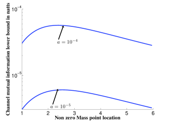
(a) Very Low SNR

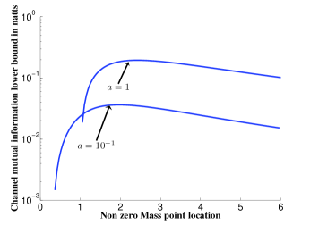
(b) Low SNR

(c) High SNR

Figure 1: Channel mutual information lower bound versus non-zero mass point for 3 SNR regimes: a) Very Low SNR, b) Low SNR and c) High SNR

In Lemma 1, the existence of a maximum for a given SNR value $a$ is guaranteed by the continuity of $I_{LB}(x_{1},a)$ and the fact that it is bounded with respect to $x_{1}$ over the interval $[\sqrt{a},\infty[$. This can be readily seen in Fig. 1 where we have plotted the lower bound $I_{LB}(x_{1},a)$ for different values of $a$. As can be seen in Fig. 1, $I_{LB}(x_{1},a)$ has a maximum for the 3 SNR regimes. The existence of such a maximum is also rigorously established in Appendix A. Clearly, as was discussed in Appendix A, the maximization (10) is reduced to solving the equation $\frac{\partial}{\partial x_{1}}I_{LB}(x_{1},a)$ for a given SNR value $a$. Ideally, an analytical solution would provide an insight as to how the non-coherent capacity and the optimal input distribution vary with the SNR. However, solving such an equation for arbitrary SNR values is very ambitious since it involves an analytical solution to a transcendental equations. Nevertheless, it is of interest to focus on the low SNR regime to get the benefit of some advantageous simplifications in order to elucidate the non-coherent capacity behavior at low SNR.

IV NON-COHERENT CAPACITY AT LOW SNR

In this section, we will use Lemma 1 to derive a fundamental analytical relation between the optimal input distribution at a low SNR regime and the particular SNR value $a$. We show in Theorem 1 that this fundamental relation holds up to an order of $a$ strictly less than 2. As is shown below, the derived relation is very useful since it allows computing the optimal input distribution for a given SNR value $a$ while providing a rigorous characterization as to how the non zero mass point locations and their probabilities vary with $a$. Moreover, the derived relation may be used to compute the exact non-coherent capacity at low SNR values.

IV-A A fundamental relation between the optimal input distribution and the SNR

We present the fundamental relation between the optimal input distribution and the SNR value in the following Theorem:

Theorem 1

At a low SNR value $a$, the optimal input probability distribution for an order of magnitude of $a$ strictly less than 2, is given by:

$$f_{x}(x)=\begin{cases}x_{1}&\text{with probability $p_{1}=\frac{a}{x_{1}^{2}}$},\\ 0&\text{with probability $p_{0}=1-p_{1}$},\end{cases}$$ (12)

where $x_{1}$ is the solution of the equation:

$$x_{1}^{2}-(1+x_{1}^{2})\ln(1+x_{1}^{2})-\pi\left(\frac{a}{x_{1}^{2}+x_{1}^{4}}\right)^{\frac{1}{x_{1}^{2}}}\csc{\left(\frac{\pi}{x_{1}^{2}}\right)}\left[1+x_{1}^{2}-\pi\cot{\left(\frac{\pi}{x_{1}^{2}}\right)}+\ln{\left(\frac{a}{x_{1}^{2}+x_{1}^{4}}\right)}\right]=0.$$ (13)

Furthermore, the non-coherent channel capacity is given by:

$$C(a,x_{1})=a-a\cdot\frac{\ln{(1+x_{1}^{2})}}{x_{1}^{2}}-a^{1+\frac{1}{x_{1}^{2}}}\cdot\frac{\pi\csc{\left(\frac{\pi}{x_{1}^{2}}\right)}\left(\frac{1}{x_{1}^{2}+x_{1}^{4}}\right)^{\frac{1}{x_{1}^{2}}}}{1+x_{1}^{2}}$$ (14)

Proof:

For convenience, the proof is presented in Appendix B. ∎

Clearly, (13) is also a transcendental equation, for which determining an analytical solution is a very tedious task. Although it is very involved to derive an analytical solution of (13) in the form of $x_{1}=f(a)$, it is of interest from an engineering point of view, to resolve (13) numerically and obtain the optimal $x_{1}$ for a given SNR value $a$. One may then get the value of the non-coherent capacity by replacing in (14) the obtained value of $x_{1}$. Moreover, (13) provides some insight on the behavior of $x_{1}$ as $a$ tends toward zero. For example, using (13), one may determine the limit of $x_{1}$ as $a$ tends toward zero. To see this, let $M$ be this limit and let us assume that $M$ is finite. From Appendix B, we know that for the optimal input distribution, the non-zero mass point location $x_{1}$ is greater than one. Thus, its limit as $a$ tends toward zero is greater or equal than one $M\geq 1$. Then, taking the limits on both sides of (13) as $a$ goes to zero yields:

$$M^{2}-(1+M^{2})\ln{(1+M^{2})}=0.$$ (15)

That is, if $M$ is finite, it would be equal to zero, the unique solution to (15), but this is impossible since $M\geq 1$. Hence, consistently with [6, 13], $\underset{a\rightarrow 0}{\lim}x_{1}=\infty$ . Furthermore, we have found that (13) may be written in a more convenient way as:

$$a=\exp{\left[x_{1}^{2}W\bigl{(}k,\varphi{(x_{1})}\bigr{)}-x_{1}^{2}+\pi\cot{\bigl{(}\frac{\pi}{x_{1}^{2}}\bigr{)}}+\ln{(x_{1}^{2})}+\ln{(1+x_{1}^{2})}-1\right]},$$ (16)

with $k=-1$ if $a\leq a_{0}$ and $k=0$ elsewhere, and where $W{(\cdot,\cdot)}$ is the Lambert function, with $\varphi{(x)}$ given by:

$$\varphi{(x)}=-\frac{\sin{(\frac{\pi}{x^{2}})}(-x^{2}+\ln{(1+x^{2})}+x^{2}\ln{(1+x^{2})})}{\pi x^{2}}\cdot\exp{\left(\frac{-\pi\cot{\left(\frac{\pi}{x^{2}}\right)}}{x^{2}}+1+\frac{1}{x^{2}}\right)}.$$ (17)

Also, $a_{0}$ is the solution of (13) for $x_{1}=x_{0}$, where $x_{0}$ is the root of the equation $\varphi{(x)}=-\frac{1}{e}$. The number $-\frac{1}{e}$ comes out in our analysis from the fact that it is the unique point shared by the principal branch of the Lambert function $W(0,x)$ and the branch with $k=-1$, $W(-1,x)$. That is $W(0,-\frac{1}{e})=W(-1,-\frac{1}{e})$. This guarantees the continuity of $a$ in (16) for all $x_{1}$ values. Numerically, we have found that $a_{0}=0.0582$ and $x_{0}=\sqrt{3.93388}$. Hence, (16) may also be viewed as a fundamental relation between the optimal input distribution and $a$ for discrete-time non-coherent memoryless Rayleigh fading channels at low SNR. On the other hand, (16) provides the global answer as to how the non-zero mass point location of the optimal on-off signaling and the SNR are linked together. For this purpose, a simple analysis of (16) has been done and some important results are recapitulated in the following corollary.

Corollary 1

At low SNR, we have:

1. For all $a\leq a_{0}$, $a_{0}=0.0582$, $a$ is an decreasing function with respect to $x_{1}$ and for all $a>a_{0}$, $a$ is an increasing function of $x_{1}$.

2. For all $a$, $x_{1}\geq x_{0}$, where $x_{0}=\sqrt{3.93388}$.

3. $\underset{x_{1}\rightarrow\infty}{\lim}{a}=0$.

Corollary 1 agrees with [6] where it was shown using computer simulation that the non-zero mass point location passes through a minimum before moving upward. However, by specifying the edge point $(x_{0},a_{0})$, Corollary 1 gives a more precise characterization concerning this peculiar behavior of the non-zero mass point locations. Furthermore, Corollary 1 also refines the lower bound on $x_{1}$, $x_{1}>1$ and derives $x_{0}$ as an improved lower bound on the non-zero mass point location at low SNR. Moreover, from (16), we may write:

$$\ln{(a)}+x_{1}^{2}=x_{1}^{2}W\bigl{(}k,\varphi{(x_{1})}\bigr{)}+\pi\cot{\bigl{(}\frac{\pi}{x_{1}^{2}}\bigr{)}}+\ln{(x_{1}^{2})}+\ln{(1+x_{1}^{2})}-1.$$ (18)

It is then easy to check that the right hand side (RHS) of (18) is a decreasing function of $x_{1}$ for $x_{1}<x_{0}$, which yields an upper bound on $x_{1}$:

$$x_{1}^{2}\leq-\ln{(a)}+\xi_{0},$$ (19)

where $\xi_{0}=\ln{(a_{0})}+x_{0}^{2}$, which is again consistent with the upper bound derived in [13]. Note that the upper bound (19) is valid for all $a\leq a_{0}$ whereas the upper bound provided in [13] holds for $a\ll a_{0}$ for which $\xi_{0}$ is negligible. On the other hand, combining (19) and the lower bound on $x_{1}$ provided in Corollary 1 one may obtain:

$$a^{\alpha}x_{0}^{2}\leq a^{\alpha}x_{1}^{2}\leq a^{\alpha}(\xi_{0}-\ln{(a)}).$$ (20)

for all $\alpha>0$. That is:

$$\underset{a\rightarrow 0}{\lim}{\bigl{(}a^{\alpha}x_{1}^{2}\bigr{)}}=0,$$ (21)

which means that $a^{\alpha}$ tends toward zero faster than $x_{1}^{2}$ does toward infinity. This result may also be used to gain further insight on the capacity behavior at low SNR. For instance, from (14), we may write the non-coherent capacity as:

$$C(a)=a+\textit{o}(a),$$ (22)

where $\textit{o}(a)=-a\cdot\frac{\ln{(1+x_{1}^{2})}}{x_{1}^{2}}-a^{1+\frac{1}{x_{1}^{2}}}\cdot\frac{\pi\csc{\left(\frac{\pi}{x_{1}^{2}}\right)}\left(\frac{1}{x_{1}^{2}+x_{1}^{4}}\right)^{\frac{1}{x_{1}^{2}}}}{1+x_{1}^{2}}$, meaning that the non-coherent capacity varies linearly with $a$ at low SNR and hence non-coherent communication at low SNR may be qualified as energy efficient communication.

IV-B Energy efficiency and non-coherence penalty

In general, the capacity of a channel including a Gaussian channel and a Rayleigh channel varies linearly at low SNR [13]. The difference between these channels in terms of capacity can only be explained by the sub-linear term $\textit{o}(a)$ in (22). The sub-linear term has been defined in [13] as:

$$\Delta(a):=a-C(a).$$ (23)

At low SNR, the sub-linear term $\Delta(a)$ is also related to the energy-efficiency. let $E_{n}$ be the transmitted energy in Joules per information nat, then we have:

$$\frac{E_{n}}{\sigma_{w}^{2}}\cdot C(a)=a.$$ (24)

Using (23), we can write:

$$\frac{E_{n}}{\sigma_{w}^{2}}=\frac{1}{1-\frac{\Delta(a)}{a}}\approx 1+\frac{\Delta(a)}{a},$$ (25)

where the approximation holds if $\frac{\Delta(a)}{a}$ is sufficiently small. Note that if

$$\frac{\Delta(a)}{a}\rightarrow 0,$$ (26)

then from (23) and (25), we have respectively:

$$C(a) \approx a$$ (27)

$$\frac{E_{n}}{\sigma_{w}^{2}} \approx 1,$$ (28)

which implies that the highest energy efficiency of -1.59 (dB) per information bit could be theoretically achieved. For a Gaussian channel and a fading channel under the coherent assumption, the sub-linear terms are respectively given by [13]:

$$\Delta_{AWGN}(a) = \frac{1}{2}a^{2}+o(a^{2})$$ (29)

$$\Delta_{coherent}(a) = \frac{1}{2}E[\|h\|^{4}]a^{2}+o(a^{2})$$ (30)

For a non-coherent Rayleigh fading channel, the sub-linear term can be computed using (14):

$$\Delta(a)=a\cdot\frac{\ln{(1+x_{1}^{2})}}{x_{1}^{2}}+a^{1+\frac{1}{x_{1}^{2}}}\cdot\frac{\pi\csc{\left(\frac{\pi}{x_{1}^{2}}\right)}\left(\frac{1}{x_{1}^{2}+x_{1}^{4}}\right)^{\frac{1}{x_{1}^{2}}}}{1+x_{1}^{2}}.$$ (31)

Note that at very low SNR and following (31), $\frac{\Delta(a)}{a}$ converges to zero making the non-coherent Rayleigh channel also energy efficient. However, as SNR increases, the convergence of $\frac{\Delta(a)}{a}$ to zero is slower than $\frac{\Delta_{AWGN}(a)}{a}$ and $\frac{\Delta_{coherent}(a)}{a}$. This could be seen from (21) indicating that $x_{1}$ converges slower to infinity than $a$ does to zero. To illustrate this, as an example, let us calculate the value of $\frac{\Delta(a)}{a}$ for an SNR value $a=-30dB$. Following (31), we can write:

$$\frac{\Delta(a)}{a}=\frac{\ln{(1+x_{1}^{2})}}{x_{1}^{2}}+a^{\frac{1}{x_{1}^{2}}}\cdot\frac{\pi\csc{\left(\frac{\pi}{x_{1}^{2}}\right)}\left(\frac{1}{x_{1}^{2}+x_{1}^{4}}\right)^{\frac{1}{x_{1}^{2}}}}{1+x_{1}^{2}}.$$ (32)

Solving (16) for $a=-30dB$ with respect to $x_{1}^{2}$ yields: $x_{1}^{2}\approx 4.96815$. Then, substituting this value in (32), we obtain $\frac{\Delta(a)}{a}\approx 49\%$. Note that for AWGN and coherent Rayleigh fading channels, $\frac{\Delta_{AWGN}(a)}{a}$ and $\frac{\Delta_{coherent}(a)}{a}$ are at the same order of magnitude than the SNR value in this case. It takes a lower SNR for non-coherent communication to achieve the same energy efficient as AWGN and coherent Rayleigh fading channels.

In the range of SNR values of interest, we may define the non-coherence penalty per SNR as:

$$\frac{C_{coherent}(a)-C(a)}{a}.$$ (33)

where $C_{coherent}$ is the channel capacity under coherent assumption. Now, from [13], we can write $C_{coherent}$ as:

$$C_{coherent}(a)=a+\textit{O}(a)=a+\textit{o}(a^{2-\alpha}),$$ (34)

for any $1>\alpha>0$. Recalling that the non-coherent capacity in (14) was obtained using series decomposition to an order strictly smaller than 2, then combining (14) and (34), we derive the exact non-coherence penalty per SNR up to this order:

$$\frac{C_{coherent}(a)-C(a)}{a}=\frac{C_{coherent}-C}{C_{coherent}}=\frac{\ln{(1+x_{1}^{2})}}{x_{1}^{2}}+a^{\frac{1}{x_{1}^{2}}}\cdot\frac{\pi\csc{\left(\frac{\pi}{x_{1}^{2}}\right)}\left(\frac{1}{x_{1}^{2}+x_{1}^{4}}\right)^{\frac{1}{x_{1}^{2}}}}{1+x_{1}^{2}}$$ (35)

Now using (21), dividing both sides of (35) by $a^{\alpha}$, ($\alpha>0$) and taking the limit as $a$ tends to zero yields:

$$C_{coherent}(a)-C(a)\gg a^{1+\alpha},$$ (36)

where $\gg$ means:

$$\underset{a\rightarrow 0}{\lim}\frac{C_{coherent}(a)-C(a)}{a^{1+\alpha}}=\infty.$$ (37)

Inequality (36) indicates that not only the non-coherent capacity is much greater than $a^{2}$ as was established in [1], but more precisely, it is much greater than $a^{1+\alpha}$ since $a^{1+\alpha}\gg a^{2}$, $1>\alpha>0$. Again, this result is in full agreement with [13].

In this subsection, we have discussed exact closed forms of the optimal input distribution and the non-coherent capacity based on the fundamental relation (13) or equivalently (16). However, one may be interested in deriving simpler lower and upper bounds on these quantities in order to better understand how they vary with the SNR value $a$. This is discussed next.

IV-C Upper and lower bounds on the non-coherent capacity

Considering (16), since we are interested in the low SNR regime, we assume for simplicity that $a\leq a_{0}$. Thus the Lambert function in (16) is the branch with $k=-1$, that is $W(-1,x)$. A lower bound on the non-coherent capacity is easily obtained by combining (19) and (14) and will be referred to as $C_{LB}(a)$. We now derive the lower bound on the optimal non-zero mass point location and the upper bound on the non-coherent capacity in Theorem 2.

Theorem 2

At low SNR values $a$, a lower bound on the optimal non-zero mass point location is given by:

$$x_{1,LB}=\frac{y}{\sqrt{-W\Biggl{(}-1,\varphi{\Bigl{(}\frac{y}{-\ln{\bigl{(}-\varphi{(y)}\bigr{)}}}\Bigr{)}}\Biggr{)}}},$$ (38)

where $y=\sqrt{1+\ln{\frac{1}{a}}}$. Furthermore, an upper bound on the non-coherent capacity can be obtained from (14) as:

$$C_{UB}(a)=C(a,x_{1,LB})$$ (39)

Proof:

For convenience, the proof is presented in Appendix C. ∎

V Numerical Results and Discussion

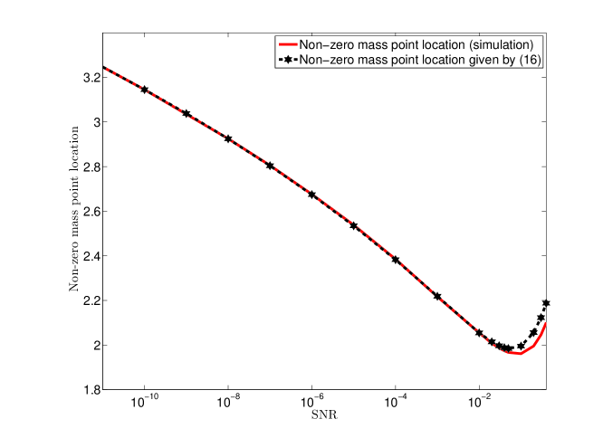
Figure 2: Location of non-zero mass point versus the SNR value $a$ (linear).

The curves in Fig. 2 show respectively, the non-zero mass point location of the capacity-achieving input distribution $x_{1}$ obtained using maximization (10), and the one obtained using relation (13) or equivalently (16). As can be seen from Fig. 2, the two curves are undistinguishable at low SNR, confirming that (17) is exact at low SNR. As the SNR increases, a small discrepancy between the two curves starts to appear. This is expected since (16) holds for up to an order of magnitude strictly smaller than 2 and thus for small SNR values, (but not smaller than about $2.10^{-2}$), a discrepancy may appear. Nevertheless, even for an SNR greater than $2.10^{-2}$, the curve obtained using (16) is very instructive especially as it follows the same shape as the one obtained by simulation results. An interesting future work would be to use (17) in order to understand why a new mass point should appear as the SNR increases. It should be mentioned that the discrepancy observed in Fig. 2 may be rendered as small as desired using high order series expansion. However, the analysis would be unrewardingly too complex.

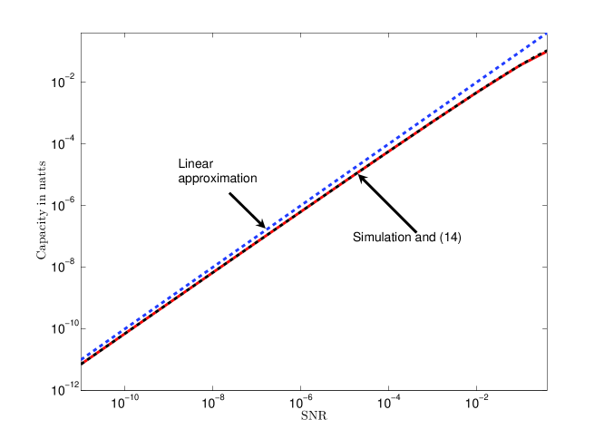
Figure 3: Non-coherent capacity versus the SNR value $a$ (linear).

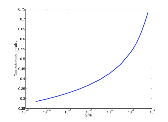
Figure 4: Non-coherentce penalty per SNR versus the SNR value $a$ (linear).

Figure 3 depicts the non-coherent capacity curves. Again, the curve obtained by computer simulation and the one obtained using (14) are undistinguishable. More interestingly, the discrepancy observed at not very low SNR values in Fig. 2 has vanished, implying that the capacity is not very sensitive to the non-zero mass point location. Also shown in Fig. 3 is the linear approximation $C(a)=a$, which is an upper bound on the capacity. As can be noticed in Fig. 3, the linear approximation follows the same shape as the exact non-coherent capacity curves at low SNR and becomes quite loose for SNR values greater than $10^{-2}$. This implies that the sub-linear term defined in (23) is much more important at these SNR values. This can be seen in Fig. 4 where we have plotted the non-coherence penalty percentage given by (35). Figure 4 confirms that there is no substantial gain in the channel knowledge in a capacity sense at very low SNR, thus indicating that non-coherent communication is almost as power-efficient as AWGN and coherent communications. As the SNR increases, a non-coherence penalty begins to appear reaching up to $70\%$.

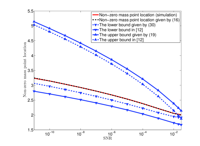
Figure 5: Exact non-zero mass point locations and the derived upper and lower bounds as well as those reported in [13] versus the SNR value $a$ (linear).

The derived upper and lower bounds on the non zero mass point locations given respectively by (19) and (38) as well as well as the bounds derived in [13] are plotted in Fig. 5 along with the exact curves at low SNR. As can be seen in Fig. 5, the upper bound in [13], albeit tighter than (19), crosses the exact curves at about $2.10^{-2}$. At these not so low SNR values, the derived bound in [13] is no longer an upper bound, consistently with our discussion in Subsection IV-A. On the other hand, the lower bound (38) is tighter than the one derived in [13] for all SNR values.

VI Conclusion

In this paper, we have addressed the analysis of the capacity of discrete-time non-coherent memoryless Rayleigh fading channels at low SNR. We have computed explicitly the channel mutual information at low SNR which is also a lower bound on the channel mutual information, albeit not necessarily at low SNR values.

Using the derived expression of the channel mutual information, we have been able to provide a fundamental relation between the non-zero mass point location of the capacity-achieving input distribution and the SNR. This fundamental relation brings the complete answer about how the optimal input distribution varies with the power constraint at low SNR. It also provides an analytical explanation on what was previously observed through computer simulation in [6] about the peculiar behavior of the non-zero mass point location at low SNR values. The exact non-coherent capacity has been derived and insights on the capacity behavior which can be gained through functional analysis has been shown.

In order to better understand how the non-zero mass point location varies with the SNR, we have also derived lower and upper bounds which have been compared to recently derived bounds. The newly derived lower bound is tighter for all SNR values of interest, whereas somewhat looser, the upper bound was shown to hold for larger SNR values.

Appendix A Proof of lemma 1

For convenience, we will use $f(x)$ instead of $f_{x}(x)$ to denote the probability density function of the random variable $x$ at the value $x$. We first prove that $I_{LB}(x;y)$ is a strictly monotonically increasing function with respect to $x_{1}$. Differentiating (9) with respect to $x_{1}$ yields

$$\frac{\partial}{\partial{x_{1}}}I_{LB}(x_{1},p_{1})=p_{1}\int_{0}^{\infty}{\frac{\partial}{\partial{x_{1}}}}f(y|x_{1})\ln{\left(\frac{f(y|x_{1})}{f(y)}\right)}dy$$ (A.40)

Differentiating (4), we obtain:

$$\frac{\partial}{\partial{x_{1}}}f(y|x_{1})=\frac{2x_{1}}{(1+x_{1}^{2})^{2}}\left[y-(1+x_{1}^{2})\right]f(y|x)$$ (A.41)

Substituting (A.41) in (A.40) yields:

$$\frac{\partial}{\partial{x_{1}}}I_{LB}(x_{1},p_{1})=\frac{2p_{1}x_{1}}{(1+x_{1}^{2})^{2}}\int_{0}^{\infty}\left[y-(1+x_{1}^{2})\right]f(y|x_{1})\ln{\left(\frac{f(y|x_{1})}{f(y)}\right)}dy$$ (A.42)

Let $g(y)$ be defined as $g(y)=\ln{\left(\frac{f(y|x_{1})}{f(y)}\right)}$. Now, we need the following lemma.

Lemma 2

Let $f(y)$ be a probability density function with mean $m$. If $g(y)$ is a strictly monotonically increasing function then

$$\int{(y-m)f(y)g(y)}>0$$ (A.43)

Proof:

The proof follows along similar lines as Lemma 1 in [6]. ∎

To apply Lemma 2, it is sufficient to note that

$$\frac{f(y)}{f(y|x_{1})}=p_{1}+p_{0}(1+x_{1}^{2})\exp{\left[y\left(\frac{1}{1+x_{1}^{2}}-1)\right)\right]}$$ (A.44)

is strictly decreasing with respect to $y$ because the exponent of the exponential function is negative, therefore $\frac{f(y|x_{1})}{f(y)}$ is strictly increasing and so is $g(y)$. Finally, using the fact that $(1+x_{1}^{2})$ is the mean of $f(y|x_{1})$ and applying Lemma 2 to (A.42), we obtain:

$$\frac{\partial}{\partial{x_{1}}}I_{LB}(x_{1},p_{1})>0,$$ (A.45)

which means that $I_{LB}(x_{1},p_{1})$ is strictly increasing with respect to $x_{1}$. Consequently, the average power constraint holds with equality. That is $E[x^{2}]=p_{1}x_{1}^{2}=a$. Hence (8) is equivalent to:

$$\begin{cases}C_{LB}=\underset{x_{1}\geq\sqrt{a}}{\max}{I_{LB}(x_{1},p_{1})}\\ p_{1}x_{1}^{2}=a.\end{cases}$$ (A.46)

Next, we prove the existence of the maximum in (A.46). Clearly, $I_{LB}(x_{1},p_{1})$ is now a function of $x_{1}$ and $a$ since $p_{1}x_{1}^{2}=a$. That $x_{1}\geq\sqrt{a}$ follows automatically from the fact that $p_{1}\leq 1$. On the other hand, $I_{LB}(x_{1},p_{1})$ in (9) is positive-definite and continue with respect to $x_{1}$ and $p_{1}$ and thus so is $I_{LB}(x_{1},a)$ for a given SNR value $a$. Moreover $I_{LB}(x_{1},a)$ is upper-bounded over the interval $[\sqrt{a},\infty[$ otherwise, one would have, for some SNR value, say $a^{0}$ :

$$\forall\ \epsilon\ >0,\quad\exists\ x_{1}^{0}\ >\ \sqrt{a^{0}}\quad|\quad I_{LB}(x_{1}^{0},a^{0})\ >\ \epsilon.$$ (A.47)

But this statement also means that the channel mutual information-an upper bound on $I_{LB}(x_{1},a^{0})$- is unbounded for $a^{0}$ which contradicts the fact that the capacity exists for all SNR values as proven in [6]. Hence, $I_{LB}(x_{1},a)$ is necessarily upper-bounded. Furthermore, the continuity of $I_{LB}(x_{1},a)$ over $[\sqrt{a},\infty[$ implies that the upper-bound is either achieved at a finite value $x_{1}$ or at $\infty$. The last case is however impossible. To see this, it is sufficient to observe that for a given $a$, as $x_{1}$ goes to infinity, $p_{1}$ tends toward zero. Thus following (9), $\underset{x_{1}\rightarrow\infty}{\lim}I_{LB}(x_{1},a)=I_{LB}(\infty,0)=0$, and consequently $I_{LB}(x_{1},a)=0$ for all $x_{1}\in[\sqrt{a},\infty[$ which is impossible since the discrete input distribution $x$ and the output $y$ are dependent. That is, the upper bound is achieved at a finite value $x_{1}$ and this proves the existence of the maximum in (A.46). Moreover, since the maximum is not at the borders of $[\sqrt{a},\infty[$, we necessarily have at the maximum $\frac{\partial}{\partial x_{1}}I_{LB}(x_{1},a)=0$.

Finally, in order to prove (11), we directly compute the lower bound $I_{LB}(x_{1},p_{1})$ from (9):

$$I_{LB}(x_{1},p_{1}) = \underbrace{p_{0}\int_{0}^{\infty}f(y|0)\ln{(f(y|0))}dy}_{I_{1}}-\underbrace{p_{0}\int_{0}^{\infty}f(y|0)\ln{(f(y))}}_{I_{2}}$$ (A.48)

$$+\underbrace{p_{1}\int_{0}^{\infty}f(y|x_{1})\ln{(f(y|x_{1}))}}_{I_{3}}-\underbrace{p_{1}\int_{0}^{\infty}f(y|x_{1})\ln{(f(y))}}_{I_{4}}$$

$I_{1}$ and $I_{3}$ may be easily computed:

$$I_{1}=p_{0}\int_{0}^{\infty}e^{-y}\ln{(e^{-y})}dy=-p_{0}=1-p_{1}$$ (A.49)

$$I_{3} = p_{1}\int_{0}^{\infty}\frac{1}{1+x_{1}^{2}}e^{-\frac{y}{1+x_{1}^{2}}}\ln{\left(\frac{1}{1+x_{1}^{2}}e^{-\frac{y}{1+x_{1}^{2}}}\right)}dy$$ (A.50)

$$= -p_{1}\left(1+\ln{(1+x_{1}^{2})}\right)$$

$$I_{2} = p_{0}\int_{0}^{\infty}e^{-y}\ln{\left(p_{0}e^{-y}+\frac{p_{1}}{1+x_{1}^{2}}e^{-\frac{y}{1+x_{1}^{2}}}\right)}dy$$ (A.51)

$$= \underbrace{\int_{0}^{\infty}p_{0}e^{-y}\ln{\left(p_{0}e^{-y}\right)}dy}_{I_{21}}+\underbrace{\int_{0}^{\infty}p_{0}e^{-y}\ln{\left(1+\frac{p_{1}}{p_{0}(1+x_{1}^{2})}e^{\left(1-\frac{1}{1+x_{1}^{2}}\right)y}\right)}dy}_{I_{22}}$$

$I_{21}$ can be easily computed:

$$I_{21}=p_{0}\left[\ln{(p_{0})}-1\right]$$ (A.52)

In order to compute $I_{22}$, let $\alpha=1+x_{1}^{2}$ and $\beta=\frac{p_{1}}{p_{0}\alpha}=\frac{p_{1}}{(1-p_{1})\alpha}$. Thus, $I_{22}$ may be written:

$$I_{22} = \frac{p_{0}\alpha}{\alpha-1}\int_{1}^{\infty}t^{\frac{1-2\alpha}{\alpha-1}\ln{(1+\beta t)}}dt$$ (A.53)

$$= \frac{p_{0}\alpha}{\alpha-1}\left\{\left[\frac{1-\alpha}{\alpha}t^{-\frac{\alpha}{\alpha-1}}\ln{(1+\beta t)}\right]_{1}^{\infty}-\frac{1-\alpha}{\alpha}\beta\int_{1}^{\infty}\frac{t^{-\frac{\alpha}{\alpha-1}}}{1+\beta t}dt\right\}$$

The integral on the RHS of (A.53) may be computed as [15]:

$$\int_{1}^{\infty}\frac{t^{-\frac{\alpha}{\alpha-1}}}{1+\beta t}dt=\frac{\alpha-1}{\alpha\beta}\cdot{}_{2}F_{1}\left(1,1+\frac{1}{\alpha-1},2+\frac{1}{\alpha-1},-\frac{1}{\beta}\right)$$ (A.54)

Substituting (A.54) in (A.53), we obtain:

$$I_{22}=p_{0}\left[\ln{(1+\beta)}+\frac{\alpha-1}{\alpha}{}_{2}F_{1}\left(1,1+\frac{1}{\alpha-1},2+\frac{1}{\alpha-1},-\frac{1}{\beta}\right)\right],$$ (A.55)

and thus combining (A.51), (A.52) and (A.55), yields:

$$I_{2}=p_{0}\left[\ln{(p_{0})}-1\right]+p_{0}\left[\ln{(1+\beta)}+\frac{\alpha-1}{\alpha}\cdot{}_{2}F_{1}\left(1,1+\frac{1}{\alpha-1},2+\frac{1}{\alpha-1},-\frac{1}{\beta}\right)\right].$$ (A.56)

The integral $I_{4}$ may be computed similarly. We skip the details and give below the final result:

$$I_{4}=p_{1}\ln{(p_{0})}-p_{1}\alpha+p_{1}\left[\ln{(1+\beta)}+(\alpha-1)\cdot{}_{2}F_{1}\left(1,\frac{1}{\alpha-1},1+\frac{1}{\alpha-1},-\frac{1}{\beta}\right)\right].$$ (A.57)

Following (A.48), (A.49), (A.50), (A.56), (A.57) and using the fact that:

$${}_{2}F_{1}\left(1,\frac{1}{\alpha-1},1+\frac{1}{\alpha-1},-\frac{1}{\beta}\right)+\frac{1-p_{1}}{p_{1}}\cdot{}_{2}F_{1}\left(1,1+\frac{1}{\alpha-1},2+\frac{1}{\alpha-1},-\frac{1}{\beta}\right)=1,$$ (A.58)

we obtain:

$$I_{LB}(x_{1},p_{1}) = -\ln{(1-p_{1})}+p_{1}\left(x_{1}^{2}-\ln{(1+x_{1}^{2})}\right)-\ln{(1+\beta)}$$ (A.59)

$$-\frac{p_{1}(\alpha-1)}{\alpha}\left[(\alpha-1)\cdot{}_{2}F_{1}\left(1,\frac{1}{\alpha-1},1+\frac{1}{\alpha-1},-\frac{1}{\beta}\right)+1\right].$$

Combining (A.59) and (A.46) yields (11) which completes the proof of Lemma 1.

Appendix B Proof of theorem 1

At low SNR, a discrete input distribution with two mass points, one of them located at zero, achieves the non-coherent capacity [6]. That $p_{1}=a/x_{1}^{2}$ was proven in Appendix A. Therefore, (12) is true. To derive (13), it is a matter of series expansion calculus.

Before proceeding, it should be reminded that for the optimal input distribution given in Theorem 1, the non-zero mass point location $x_{1}$ is greater than 1 $(x_{1}>1)$ [6, 13]. Then, series expansion of (11) to the second order, around the point $(x_{1},a)=(x_{1},0)$, where $x_{1}$ is an arbitrary real greater than one, can be obtained using Mathematica:

$$I_{LB}(x_{1},a) = \biggl{(}(1-\frac{\log(1+x_{1}^{2})}{x_{1}^{2}})a+\frac{1}{2(x_{1}^{2}-1)}a^{2}+\textit{o}{(a^{2})}\biggr{)}$$ (B.60)

$$-a^{\frac{1}{x_{1}^{2}}}\biggl{(}\pi x_{1}^{2}\biggl{(}x_{1}^{2}(1+x_{1}^{2})\biggr{)}^{-\frac{1+x_{1}^{2}}{x_{1}^{2}}}\csc{\biggl{(}\frac{\pi}{x_{1}^{2}}\biggr{)}}a$$

$$+\frac{\pi\biggl{(}x_{1}^{2}(1+x_{1}^{2})\biggr{)}^{-\frac{1+x_{1}^{2}}{x_{1}^{2}}}\csc{\biggl{(}\frac{\pi}{x_{1}^{2}}}\biggr{)}}{x_{1}^{2}}a^{2}+\textit{o}{(a^{2})}\biggr{)},$$

where the symbol $\circ{(a^{n})}$ represents a function say $g(x_{1},a)$, such that $\underset{a\rightarrow 0}{\lim}\frac{g(x_{1},a)}{a^{n}}=0$. Since $x_{1}>1$, then there exists $\epsilon>0$ such that $1+\frac{1}{x_{1}^{2}}<2-\epsilon$. Thus, (A.40) may be written as:

$$I_{LB}(x_{1},a)=\biggl{(}1-\frac{\log(1+x_{1}^{2})}{x_{1}^{2}}\biggr{)}a-\pi x_{1}^{2}\biggl{(}x_{1}^{2}(1+x_{1}^{2})\biggr{)}^{-\frac{1+x_{1}^{2}}{x_{1}^{2}}}\csc{\biggl{(}\frac{\pi}{x_{1}^{2}}\biggr{)}}a^{1+\frac{1}{x_{1}^{2}}}+\textit{o}{(a^{2-\epsilon})},$$ (B.61)

which represents series expansion to an order strictly less than 2. Up to this order, we may make some abuse of notation, drop the term $\textit{o}{(a^{2-\epsilon})}$ and write (B.61) as:

$$I_{LB}(x_{1},a)=\biggl{(}1-\frac{\log(1+x_{1}^{2})}{x_{1}^{2}}\biggr{)}a-\pi x_{1}^{2}\biggl{(}x_{1}^{2}(1+x_{1}^{2})\biggr{)}^{-\frac{1+x_{1}^{2}}{x_{1}^{2}}}\csc{\biggl{(}\frac{\pi}{x_{1}^{2}}\biggr{)}}a^{1+\frac{1}{x_{1}^{2}}}.$$ (B.62)

Maximizing (A.42) with respect to $x_{1}>1$ is equivalent to:

$$\min_{x_{1}>1}\Biggl{[}\frac{\log(1+x_{1}^{2})}{x_{1}^{2}}+\pi x_{1}^{2}\biggl{(}x_{1}^{2}(1+x_{1}^{2})\biggr{)}^{-\frac{1+x_{1}^{2}}{x_{1}^{2}}}\csc{\biggl{(}\frac{\pi}{x_{1}^{2}}\biggr{)}}a^{1+\frac{1}{x_{1}^{2}}}\Biggr{]}.$$ (B.63)

As was proven in Appendix A, at the maximum, we have necessarily $\frac{\partial}{\partial x_{1}}I_{LB}(x_{1},a)=0$. Differentiating (B.63) with respect to $x_{1}$ yields (13). Finally, (14) follows from (B.62). This completes the proof of Theorem 1.

Appendix C Proof of theorem 2

For $a<a_{0}$ and $x_{1}>x_{0}$, (16) may be written as:

$$a(x_{1})=\exp{\bigl{[}x_{1}^{2}W\bigl{(}-1,\varphi{(x_{1})}\bigr{)}-x_{1}^{2}+\pi\cot{\bigl{(}\frac{\pi}{x_{1}^{2}}\bigr{)}}+\ln{(x_{1}^{2})}+\ln{(1+x_{1}^{2})}-1\bigr{]}}.$$ (C.64)

Moreover, it is easy to check that $a$ in (C.64) is a decreasing function with respect to $x_{1}$ and that:

$$-x_{1}^{2}+\pi\cot{\bigl{(}\frac{\pi}{x_{1}^{2}}\bigr{)}}+\ln{(x_{1}^{2})}+\ln{(1+x_{1}^{2})}-1>1,$$ (C.65)

for $x_{1}>x_{0}$. Thus, using (C.64) and (C.65), we have:

$$a(x_{1})>a_{lb}(x_{1})=\exp{\bigl{[}x_{1}^{2}W\bigl{(}-1,\varphi{(x_{1})}\bigr{)}+1\bigr{]}},$$ (C.66)

where $a_{lb}(x_{1})$ is a lower bound on $a(x_{1})$. Since $a_{lb}(x_{1})$ is also a decreasing function with respect to $x_{1}$, then for a low SNR value $a$, (C.66) may be seen as a lower bound on the optimal non-zero mass point location $x_{1}$ and we equivalently have:

$$x_{1}>x_{1,lb},$$ (C.67)

where $x_{1,lb}$ is the solution of $a_{lb}(x_{1})=a$. Next, we derive a lower bound on $x_{1,lb}$.

Let us fixe a low SNR value $a<a_{0}$ and consider the function on the RHS of (C.66) written for simplicity as:

$$a=\exp{\bigl{[}x_{1,lb}^{2}W\bigl{(}-1,\varphi{(x_{1,lb})}\bigr{)}+1\bigr{]}},$$ (C.68)

or equivalently by letting $y=\sqrt{1+\ln{\bigl{(}\frac{1}{a}\bigr{)}}}$:

$$x_{1,lb}^{2}=\frac{y^{2}}{-W\bigl{(}-1,\varphi{(x_{1,lb})}\bigr{)}}.$$ (C.69)

Since $-W\bigl{(}-1,\varphi{(x_{1,lb})}\bigr{)}>1$ for $x_{1,lb}>x_{0}$, it is easy to see that $y^{2}>x_{1,lb}^{2}$. Hence, using the fact that $\varphi{(\cdot)}$ and $-W\bigl{(}-1,\cdot\bigr{)}$ are strictly increasing functions, we have:

$$x_{1,LB}^{(1)}=\frac{y}{\sqrt{-W\bigl{(}-1,\varphi{(y)}\bigr{)}}}<x_{1,lb}=\frac{y}{\sqrt{-W\bigl{(}-1,\varphi{(x_{1,lb})}\bigr{)}}},$$ (C.70)

where the superscript $(^{1})$ on the left hand side of (C.70) means a first lower bound. Next we improve the lower bound $x_{1,LB}^{(1)}$ to obtain a tighter one. But before going on, we remind this result from [16] which aims at resolving transcendental equations involving Lambert function iteratively using self-mapping techniques:

Lemma 3

For the region specified by $x<1$ and $-\frac{1}{e}<y<0$, an infinite-ladder solution to the equation:

$$y(x)=xe^{x}$$ (C.71)

is easily identified as

$$x(y)=L_{<}(y),$$ (C.72)

with the ladder $L_{<}(y)$ defined as

$$L_{<}(y)=-\ln{\Biggl{(}\frac{\ln{\frac{\ln{(\ldots)}}{-y}}}{-y}\Biggr{)}}.$$ (C.73)

Proof:

The proof and more details concerning the Lambert function can be found in [16]. ∎

Clearly, using (C.73) and the fact that the solution of (C.71) is also $x(y)=W(-1,y)$, one can obtain a simple upper bound on the Lambert function in the interval of interest:

$$W(-1,y)\leq\ln{(-y)}-\ln{\bigl{(}-\ln{(-y)}\bigr{)}}.$$ (C.74)

Since for $x_{1,lb}>x_{0}$, $\varphi{(x_{1,lb})}\in]-\frac{1}{e},0[$ and $W(-1,\varphi{(x_{1,lb})})<0$, then applying (C.74) to $\varphi{(x_{1,lb})}$ yields:

$$W(-1,\varphi{(x_{1,lb})}) \leq \ln{\bigl{(}\frac{-\varphi{(x_{1,lb})}}{-\ln{\bigl{(}-\varphi{(x_{1,lb})}\bigr{)}}}\bigr{)}}$$ (C.75)

$$\leq \ln{\bigl{(}\frac{-\varphi{(y)}}{-\ln{\bigl{(}-\varphi{(x_{1,lb})}\bigr{)}}}\bigr{)}}$$ (C.76)

$$\leq \ln{\bigl{(}-\varphi{(y)}\bigr{)}}.$$ (C.77)

Inequality (C.76) holds because $y>x_{1,lb}$ and $\varphi{(\cdot)}$ is an increasing function, likewise (C.77) follows from the fact that for $x>x_{0}$, $\varphi{(x)}>-\frac{1}{e}$ and thus $\frac{1}{-\ln{\bigl{(}-\varphi{(x)}\bigr{)}}}<1$. Moreover, (C.77) implies

$$\frac{y}{-\ln{\bigl{(}-\varphi{(y)}\bigr{)}}}\geq\frac{y}{-W(-1,\varphi{(x_{1,lb})})}=x_{1,lb}$$ (C.78)

Applying again respectively $\varphi{(\cdot)}$ and $-W(-1,\cdot)$ to both sides of (C.78) gives:

$$x_{1,LB}^{(2)}=\frac{y}{\sqrt{-W\biggl{(}-1,\varphi{\Bigl{(}\frac{y}{-\ln{\bigl{(}-\varphi{(y)}\bigr{)}}}\Bigr{)}}\biggr{)}}}\leq\frac{y}{\sqrt{-W(-1,\varphi{(x_{1,lb})})}}=x_{1,lb}.$$ (C.79)

Finally, to prove that $x_{1,LB}^{(2)}$ is tighter than $x_{1,LB}^{(1)}$, it is sufficient to note that since $\varphi{(x_{1,lb})}\in]-\frac{1}{e},0[$, $y>x_{1,lb}$ and $\varphi{(\cdot)}$ is an increasing function, then $\varphi{(y)}\in]-\frac{1}{e},0[$ and we have consequently: $y>\frac{y}{-\ln{\bigl{(}-\varphi{(y)}\bigr{)}}}$. Applying again respectively $\varphi{(\cdot)}$ and $-W(-1,\cdot)$ to this inequality yields:

$$x_{1,LB}^{(1)}=\frac{y}{\sqrt{-W\bigl{(}-1,\varphi{(y)}\bigr{)}}}\leq\frac{y}{\sqrt{-W\biggl{(}-1,\varphi{\Bigl{(}\frac{y}{-\ln{\bigl{(}-\varphi{(y)}\bigr{)}}}\Bigr{)}}\biggr{)}}}=x_{1,LB}^{(2)}.$$ (C.80)

Combining (C.79) and (C.80), we have:

$$x_{1,LB}^{(1)}\leq x_{1,LB}^{(2)}\leq x_{1,lb},$$ (C.81)

from which (38) follows by letting $x_{1,LB}^{(2)}=x_{1,LB}$. Finally, (39) may be obtained by applying (14) to $x_{1,LB}$. This completes the proof of Theorem 2.

References

- [1] Sergio Verdú, “Spectral Efficiency in the Wideband Regime,” IEEE Trans. on Information Theory, vol. 48, no. 6, pp. 1319-1343, June 2002.
- [2] Muriel Médard, “The Effect upon Channel Capacity in Wireless Communications of Perfect and Imperfect Knowledge of the Channel,” IEEE Trans. on Information Theory, vol. 46, no. 3, pp. 933-946, May 2000.
- [3] Ericson T., “A Gaussian Channel with Slow fading,” IEEE Trans. on Information Theory, vol. 16, pp. 353-356, 1970.
- [4] G. Foschini, “Layered space time architecture for wireless communication in a fading environment when using multi-element antennas,” Bell Systems Technical Journal, vol. 1, pp. 41–59, Autumn 1996.
- [5] I. E. Telatar, “Capacity of multi-antenna gaussian channels,” Europeen Trans. On Communication, vol. 10, no. 6, pp. 585–5595, Nov. 1999.
- [6] Ibrahim C. Abou-Faycal, Mitchell D. Trott and Shlomo Shamai(Shitz), “The Capacity of Discrete-Time memoryless Rayleigh-Fading Channels,” IEEE Trans. on Information Theory, vol. 47, no. 4, pp. 1290-1301, May 2001.
- [7] R. R. Perera, K. Nguyen, T.S. Pollock; and T.D. Abhayapala, “Capacity of non-coherent Rayleigh fading MIMO channels.” Communications, IEE Proceedings-, Vol.153, Iss.6, Dec. 2006 Pages:976-983
- [8] T. L. Marzetta and B. M. Hochwald, “Capacity of a mobile multiple-antenna communication link in Rayleigh flat fading ,” IEEE Trans. on Information Theory, vol. 45, no. 1, pp. 139-157, Jan. 1999.
- [9] Lizhong Zheng and David N. C. Tse “Communication on the Grassmann Manifold: A Geometric Approach to the Noncoherent multiple-antenna channel,” IEEE Trans. on Information Theory, vol. 48, no. 2, pp. 359-383, Feb. 2002.
- [10] R. S. Kennedy, Fading Dispersive Communication Channels, New York: Wiley, 1969.
- [11] I. E. Telatar and D. Tse “Capacity and Mutual Information of Wideband Multiplath Fading Channels,” IEEE Trans. on Information Theory, vol. 46, no. 4, pp. 1384-1400, July 2000.
- [12] R. G. Gallager, Information Theory and Reliable Communication, New York: Wiley, 1968.
- [13] Lizhong Zheng, David N. C. Tse and Muriel Médard “Channel Coherence in the Low-SNR Regime,” IEEE Trans. on Information Theory, vol. 53, no. 3, pp. 976-997, March 2007.
- [14] Siddharth Ray, Muriel Médard and Lizhong Zheng “On NONcoherent MIMO Channels in the Wideband Regime: Capacity and Reliability,” IEEE Trans. on Information Theory, vol. 53, no. 6, pp. 1983-2009, June 2007.
- [15] I. S. Gradshteyn and I. M. Ryzhik, Table of Integrals, Series, and Products, A. Jeffrey, Ed. Academic Press, inc, 1980.
- [16] Galen Pickett1 and Yonko Millev, “On the analytic inversion of functions, solution of transcendental equations and infinite self-mappings,” JOURNAL OF PHYSICS A: MATHEMATICAL AND GENERAL,vol. 35, pp. 4485 4494, 2002.