Magnetically-controlled velocity selection in a cold atom sample using stimulated Raman transitions

Abstract

We observe velocity-selective two-photon resonances in a cold atom cloud in the presence of a magnetic field. We use these resonances to demonstrate a simple magnetometer with sub-mG resolution. The technique is particularly useful for zeroing the magnetic field and does not require any additional laser frequencies than are already used for standard magneto-optical traps. We verify the effects using Faraday rotation spectroscopy.

I Introduction

Stimulated Raman transitions that couple atomic ground states with counterpropagating laser beams are resonant only within a narrow velocity band. This atomic velocity selection Kasevich et al. (1991) has proven to be a useful tool for a variety of experiments, including subrecoil Raman cooling Boyer et al. (2004), atom interferometry McGuirk et al. (2002), and atom velocimetry Chabé et al. (2007). Stray magnetic fields can adversely affect this process by shifting the magnetic sublevels, thereby perturbing the participating velocity bands Boyer et al. (2004); Chabé et al. (2007); Ringot et al. (2001). Conversely, when transitions occur between different magnetic sublevels of a single hyperfine level, velocity selectivity can provide an excellent measure of stray or applied magnetic fields.

Elimination of stray fields to sub-milliGauss levels is particularly important for sub-recoil cooling processes Boyer et al. (2004); Vuletić et al. (1998). Typically, these fields are nulled by Helmholtz coils along each cartesian direction. Correct compensation currents can roughly be estimated by visual indicators such as atom expansion in an optical molasses, but these cues are strongly dependent on optical alignment. Stray fields can be directly measured using, for example, Faraday spectroscopy, which provides picoTesla sensitivity Isayama et al. (1999); Smith et al. (2003); Labeyrie et al. (2001), but requires additional laser frequencies and time-resolved polarimetry. Measurement of vector magnetic fields with magneto-resistive probes has been used for active compensation of both DC and AC fields, but needs several sensors placed externally to the vacuum chamber Ringot et al. (2001).

In this paper, we describe a simple imaging technique for measuring magnetic fields with sub-milliGauss resolution using a sample of cold atoms from a point trap. The technique relies on velocity-selective two-photon resonances Kasevich et al. (1991) (VSTPR) in a magnetic field, where the two-photon resonance occurs between different magnetic sublevels within a single hyperfine level. When applied to atoms cooled in an alkali-vapor MOT, no additional laser frequencies are required, because the VSTPR pulse can be derived from the repumping laser beams. The two main requirements are 1) VSTPR beams along a horizontal axis and 2) a CCD camera whose optical axis is orthogonal to the propagation direction of the VSTPR beams.

II Background

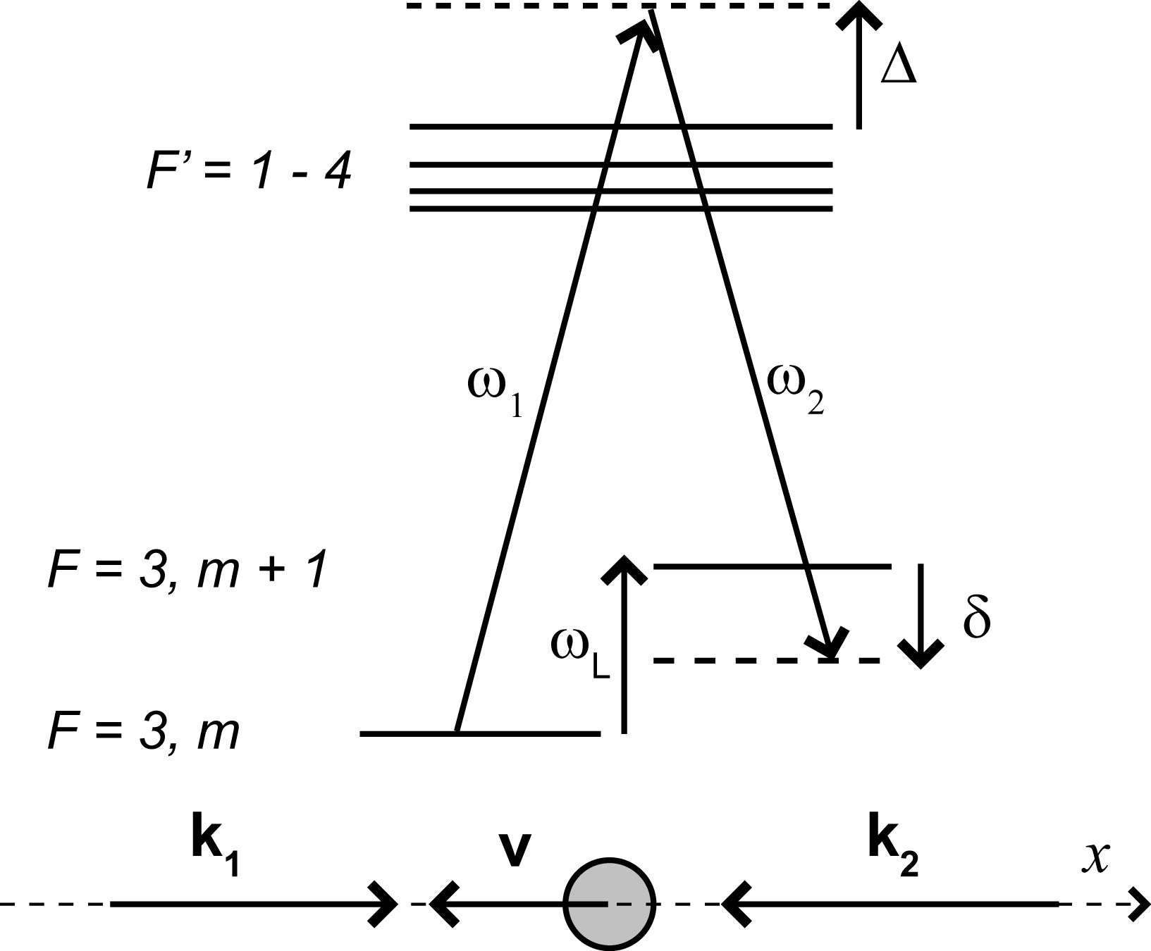
Figure 1: Relevant energy levels for the Raman transitions. Magnetic sublevels are split by the Larmor precession frequency, $\omega_{L}$. The polarization configuration is lin $\perp$ lin. The energy scale is exaggerated for clarity.

In this section, we briefly describe the process. Figure 1 shows the relevant energy levels. An atom moving with velocity v along the $x$-axis is exposed to a light field composed of two counterpropagating laser beams with wave vectors $\mathbf{k_{1}}$ and $\mathbf{k_{2}}$, where $\mathbf{k_{1}}\simeq-\mathbf{k_{2}}\simeq\mathbf{k}$ along the $x$-axis. The polarizations of the two beams are lin $\perp$ lin. For an arbitrary B-field, this polarization configuration couples $m_{f}-m_{i}=\Delta{m}=0,{\pm}1,{\pm}2$ magnetic sublevels of a single hyperfine level, where we choose our quantization axis along the magnetic field. Absorption of a photon from one beam and emission into the other results in a linear momentum change of $\pm\hbar(\mathbf{k_{1}}-\mathbf{k_{2}})\approx\pm 2\hbar\mathbf{k}=\pm 2Mv_{r}\mathbf{\hat{x}}$, where $v_{r}$ is the recoil velocity and $M$ is the mass. The one-photon detuning, $\Delta$ is chosen to be much larger than the hyperfine splittings of the upper state.

The two-photon detuning is defined here as $\delta=\omega_{1}-\omega_{2}-(\Delta{m})\omega_{L}$, where $\omega_{L}$ is the Zeeman splitting. In a small magnetic field, $\hbar\omega_{L}=g_{F}{\mu}_{B}{B}$, where $g_{F}$ is the gyromagnetic ratio, and $\mu_{B}$ is the Bohr magneton. For ⁸⁵Rb, $g_{F}{\mu}_{B}/\hbar$ = 466.74 kHz/Gauss Alexandrov et al. (2004). Two-photon resonance occurs for atoms whose velocity satisfies

$$\delta=\delta_{LS}+\delta_{D}+4\delta_{r},$$ (1)

where the two-photon Doppler shift, $\delta_{D}=2\mathbf{k}{\cdot}\mathbf{v}$, and the recoil frequency $\delta_{r}={\hbar}k^{2}/2M$. The relative light shift, $\delta_{LS}$ is a weak function of the participating magnetic sublevels, which are both in the same hyperfine ground state. Apart from $\delta_{LS}$, and with $\omega_{1}=\omega_{2}$, the resonance condition is satisfied for atoms with $\mathbf{v}=\mathbf{v_{0}}\pm{v_{r}\mathbf{\hat{x}}}$ such that $2\mathbf{k}{\cdot}\mathbf{v_{0}}=(\Delta{m})\omega_{L}$.

Throughout the duration of the VSTPR pulse, resonant atoms oscillate between the two momentum states separated by $2{\hbar}\mathbf{k}$. Because the atoms are initially confined in a point trap, an image of the atom cloud after expansion is a spatial map of the average velocity distribution, which has been perturbed by the VSTPR pulse. A freely expanding cloud has approximately a smooth Gaussian velocity spectrum along $x$ (the VSTPR beam direction), but the momentum oscillations that occur for the resonant atoms alter this average velocity distribution. Images taken along a camera direction orthogonal to $x$ record these narrow perturbations.

III Experiment Setup

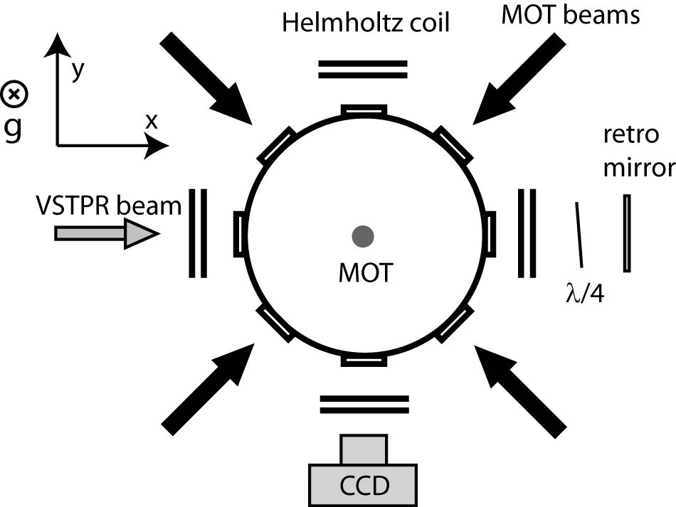
Figure 2: Experimental setup for observing VSTPR in a magnetic field.

The layout of our apparatus is shown in Fig. 2. The experiment begins with a vapor cell MOT containing 10^{7 85}Rb atoms. The MOT diameter is $\approx$500 $\mu$m and the temperature is $\approx$200 $\mu$K. The cooling beams (detuned -18 MHz from the $F$=3 - $F^{\prime}$=4 transition) are derived from an extended cavity diode laser (New Focus Vortex, model 6013) that seeds a 120 mW laser diode (Sharp GH0781JA2C). 60 mW is directed to one port of a 2 x 3 polarization maintaining (PM) fiber splitter. Each of the three output fibers carries 12 mW. The outputs are collimated using 100-mm focal length, 50mm-diameter achromats, giving 1/e² beam diameters of 24 mm. The three beams propagate along orthogonal directions and are retroreflected; one pair is vertical and the other two are in a horizontal ($x$-$y$) plane. The repump light, connecting $F=2\rightarrow F^{\prime}=3$, is derived from an independent Vortex laser that also seeds a diode. In normal MOT operation, 15 mW of repump light is coupled into the other port of the 2x3 coupler.

Our VSTPR beam is spatially filtered by PM fiber, and is collimated by a 60mm gradient-index singlet lens ($1/e^{2}$ beam waist $\omega_{0}$ = 7.5 mm). We use up to 20 mW laser power. It is retroreflected in a lin $\perp$ lin configuration. For B-field control, we use three orthogonal pairs of Helmholtz coils. The magnetic field at the atom cloud has components $B_{i}=\alpha_{i}(I_{i}-I_{0i})$ where $\alpha_{i}$ are the slopes $dB_{i}/dI_{i}$, $I_{i}$ are the applied currents, and $I_{0i}$ are the currents required for compensation along each Cartesian direction. The VSTPR beam travels horizontally along the axis of the $x$-directed coil pair. For all results in this paper, we have used a second beam derived from the repump laser as our VSTPR beam ($\Delta=3$GHz).

At time T = 0, the atoms are released from the MOT by extinguishing all laser beams and the MOT coils. The bias magnetic coils remain on. We do not perform any molasses cooling, because the large velocity spread of the hotter sample of atoms provides greater range over which velocity selection can occur. At time $T_{r}\approx 15$ ms, the VSTPR pulse is switched on for 5 ms and at $T_{i}=40$ ms, the MOT cooling and repump beams are switched on to image the expanded cloud onto the CCD camera.

IV Results

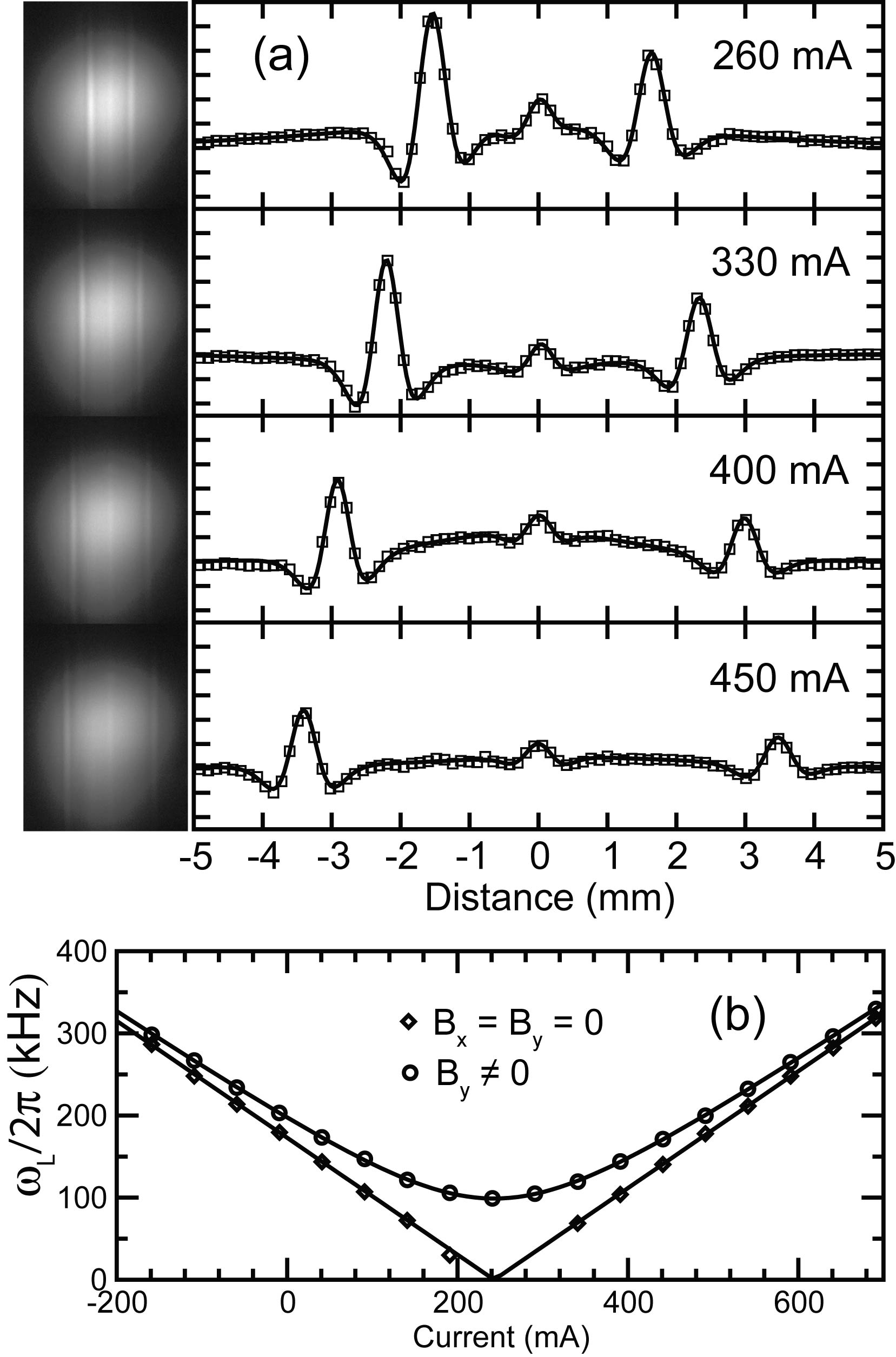
Figure 3: a) Left: Raw images of the expanded atom cloud at different Helmholtz currents after exposure to the VSTPR beams. Right: Corresponding cross-sectional profiles after background subtraction. Fits are shown as solid lines. b) Larmor precession frequency extracted from the stripe separation as a function of current in the $z$-directed coils for a nonzero $B_{y}$ field (circles) and for $B_{x}=B_{y}=0$ (diamonds). Fits shown as solid lines.

We control the magnetic field by changing the current in the Helmholtz bias coils. We first demonstrate the effect by changing the current in the $z$-directed Helmholtz coils. Fig. 3a shows typical images recorded by the CCD camera for four different current settings. The VSTPR pulse creates perturbations that appear as vertical stripes in the expanded cloud. Also shown in Fig. 3a are the cross sections after subtracting the images obtained with no VSTPR pulse. The spatial location of each peak corresponds to the average velocity class satisfying $2{\mathbf{k}\cdot}\mathbf{v_{0}}=\pm(\Delta{m})\omega_{L}$ that participated in the VSTPR process. In general, $\omega_{L}$ is a function of position due to spatially varying magnetic fields. These gradients could tip, bend, or blur the resonant stripe features. Under normal operating conditions, however, we do not observe these effects. With the B-field primarily along the $z$-axis and using lin $\perp$ lin polarizations, the VSTPR pulse mainly connects $\Delta{m}=1$ transitions. The cross-sectional profile of each vertical stripe can be estimated by several functional forms. For simplicity, we fit each peak to two Gaussian profiles such that the total area is 0, but we describe a more exact fitting function below.

In addition to the peaks corresponding to velocity classes at $\pm{v_{0}}$, there is a peak at v = 0 due to $\Delta{m}=0$ transitions that arises from the longitudinal magnetic field component. This is a useful marker for balancing the overall velocity distribution. We rarely observe features corresponding to ${\Delta}m={\pm}2$ transitions. Detailed calculations of the relative transition strengths will be published elsewhere, but in general, the strengths of the ${\Delta}m={\pm}2$ transitions are roughly two orders of magnitude smaller than those for ${\Delta}m=0,{\pm}1$ for $\Delta=3$ GHz. It is important to note that the appearance of narrow features in the expanded cloud is not the result of cooling, because there is no dissipative force. For smaller $\Delta$, on the order of the hyperfine splittings of the D2 manifold, spontaneous scattering events can lead to magnetically-induced laser cooling Sheehy et al. (1990).

The $z$-directed Helmholtz bias coils are each made of 24 gauge wire wound on an 8” vacuum flange, 1” long, and centered 5.8 cm from the MOT, producing a field of approximately 1.5 G/A. Our fits to Fig. 3 show that after 35 ms of falling time, the separations of the stripes for the 4 current settings 260 mA, 330 mA, 400 mA, and 450 mA are 3182(4) $\mu$m, 4538(4), $\mu$m, 5902(4) $\mu$m, and 6873(4) $\mu$m. The listed errors are statistical. Our leading systematic source of multiplicative error is the pixel calibration on the camera of $\approx$0.2%. In section VI, we briefly describe a second calibration procedure that removes pixel calibration errors. The 4 $\mu$m error in stripe separation corresponds to an error of  300 $\mu$G. Note that the error in magnetic field will be explicitly dependent on the atom species through $g_{F}$ and the VSTPR wavelength.

The scalar magnetic field measurements for several current settings are shown in Fig. 3b. Because the stripe separation is proportional to ${(B_{x}^{2}+B_{y}^{2}+B_{z}^{2})^{1/2}}$, a plot of $\omega_{L}$ versus the current in the $z$-directed bias coil traces a hyperbola, the minimum of which determines the field component perpendicular to $z$ and the compensation current $I_{0z}$. We show two cases, one with nonzero $B_{y}$, and one for the case in which $B_{x},B_{y}$ have been zeroed. From a fit to these plots, we extract $\alpha_{z}=1.524(2)$ G/A and $I_{0z}$ = 243.1(2) mA, which corresponds to a compensation level of 300 $\mu$G. In practice, it is simple to zero the magnetic field by viewing real-time images of the expanded cloud and adjusting the currents along each axis for minimum stripe separation. We note that when the total magnetic field is close to zero, the stripes begin to overlap and are no longer resolved. Compensation is achieved when the overlap is maximized, resulting in a single narrow feature. In our experience, this real-time adjustment of the stripe separation results in compensation to milliGauss levels without any data analysis.

The visibility of the stripe features is dependent on a few factors. First, since the image on the CCD camera is a convolution of the initial MOT size with the velocity distribution, the contrast increases for trapped samples with smaller physical dimensions. Optimally, the imaging should be performed after the cloud has expanded enough that two velocity classes separated by $2{\hbar}\mathbf{k}/M$ can be resolved. If the initial MOT has a radius R, this means that the imaging should be performed after a time $R/v_{rec}$ from the release of the atoms from the trap. In practice, the features are easily observed with imaging times significantly less because the effect does not require that the recoil velocities be resolved, only that perturbations to the average velocity distribution can be observed.

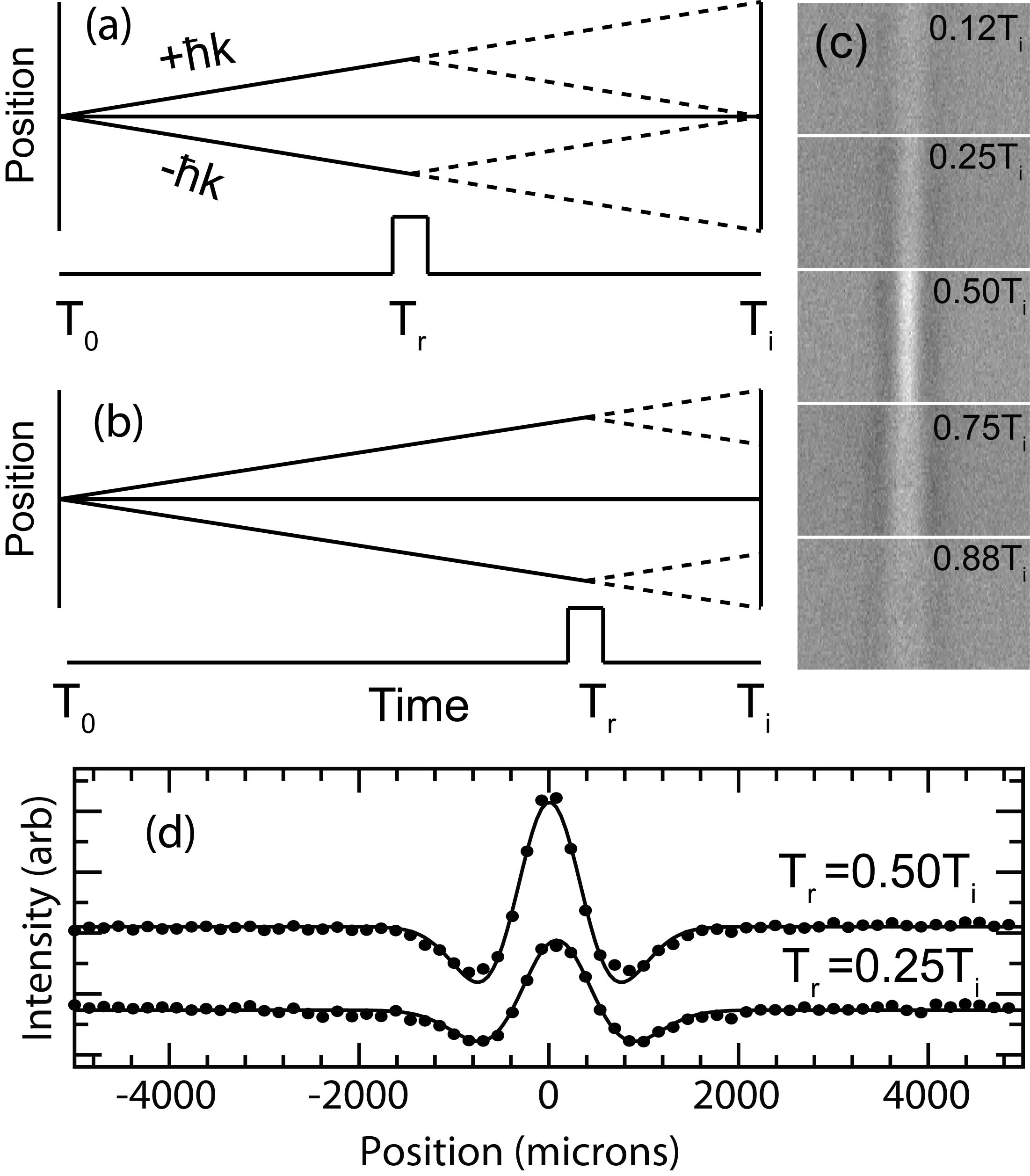
Figure 4: a) Importance of timing of the VSTPR pulse. An atom moving with ${\hbar}k$ has its momentum reversed at $T_{r}$. If this pulse occurs at $T_{i}/2$, atoms initially having ${\pm}{\hbar}k$ are overlapped at $T_{i}$. b) If the pulse arrives later or earlier, contrast is reduced. c) Pictures of a single stripe using different $T_{r}$, showing optimum contrast at $T_{i}/2$. d) Stripe cross-sections for $T_{r}=0.5T_{i}$ and $T_{r}=0.25T_{i}$, along with fits using Equation 2 (solid line).

Other parameters that control the visibility of the stripes are the duration and timing of the VSTPR pulse. Because this measurement is time-averaged over the duration of the pulse, shorter pulses reduce blurring effects due to time-varying fields. Furthermore, if applied at $T_{r}=T_{i}/2$ they can maximize stripe contrast. Figure 4a shows the effect on stripe contrast as a function of $T_{r}$ for atoms in zero field. An atom initially at the origin will return to the origin if its momentum is reversed by a $\pi$-pulse at $T_{i}/2$. For $\Delta{T}=T_{r}-T_{i}/2\neq 0$, the atoms are still deflected, but the atoms with initial momenta of ${\pm}{\hbar}k$ no longer spatially overlap at $T_{i}$ (Fig. 4b). In Fig. 4c, we show this effect experimentally using VSTPR pulse durations of 200 ${\mu}$sec at different $T_{r}$. This simple geometrical picture suggests an approximate functional form for the background-subtracted stripe cross section under these conditions:

$$Y(x) = G(x_{0}-2v_{r}\Delta{T})+G(x_{0}+2v_{r}\Delta{T})$$ (2)

$$- G(x_{0}-v_{r}T_{i})-G(x_{0}+v_{r}T_{i})$$

where $G(x_{0})$ is a Gaussian centered at $x_{0}$. In Fig. 4d, we show fits when $T_{r}=0.5T_{i}$ and $T_{r}=0.25T_{i}$. For all other data presented in this manuscript, we used pulse durations of 5 msec. Although AC magnetic fields were not compensated, these longer pulses showed no measurable broadening in our experiment. The $\pi$-pulse duration depends on the particular magnetic sublevels involved, so for our spin-unpolarized sample we generally choose a pulse duration that provides consistently strong signals over a broad range of Raman pulse intensities. For a typical VSTPR beam intensity of 10 mW/cm², the resonant 2-photon Rabi frequency is ${\approx}2\pi\times$10 kHz.

V Comparison with Faraday Spectroscopy

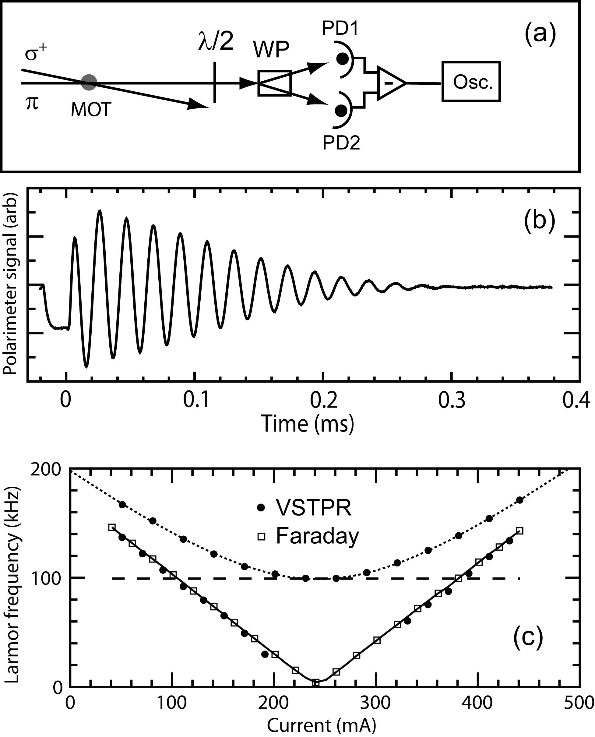
Figure 5: a) Schematic of Faraday spectroscopy setup. WP: Wollaston prism. b) Typical Faraday signal. c) Comparison of magnetic field measurement with VSTPR (circles) and with Faraday spectroscopy (squares) for similar conditions as Fig. 3b. Solid line is a fit to the Faraday data. Dotted line is a fit to the VSTPR data. Dashed line indicates the minimum of the hyperbola as measured by Faraday spectroscopy.

We have verified this VSTPR technique by using Faraday rotation spectroscopy to measure the magnetic field Isayama et al. (1999); Smith et al. (2003); Labeyrie et al. (2001). To perform these measurements, an additional pair of laser beams is used along the $x$-axis (Fig. 5a). The atoms are optically pumped into the $F=3,m_{F}=3$ stretched state (in the $x$-basis) by a 100 $\mu$s $\sigma^{+}$ pulse connecting $F=3\rightarrow F^{\prime}=3$. This beam contains a small amount of repumper light to keep the atoms in F=3. When this light is extinguished, the atoms begin precessing freely. A linearly polarized probe beam with $\simeq$100 $\mu$W and waist $\omega_{0}=500{\mu}$m passes through the atom cloud to a simple polarimeter consisting of a Wollaston prism that splits the probe beam into two orthogonal polarization states that are detected by a balanced photodetector Hobbs (1997). We make these measurements at the same time delay as the VSTPR measurements. A typical Faraday signal is shown in Fig. 5b. The comparison of the VSTPR and Faraday techniques is shown in Fig. 5c. Because we cannot compare Faraday and stripe measurements near zero field where the stripes are unresolved, we show in Fig. 5c the stripe data with and without a transverse field along $y$. This transverse field allows a stripe measurement at $I_{0z}$, which is in good agreement with the Faraday measurement (dashed line in Fig. 5c). From the Faraday measurements with no transverse field, also shown in this figure, we derive $\alpha_{z}=1.547(3)$ G/A and $I_{0z}=242.5(1)$ mA, both of which agree well with the VSTPR technique.

VI Calibration

To obtain correct values of the magnetic field, the stripe separation must be carefully measured. Without calibration, the technique is still useful for determining the $I_{0i}$ of each coil by simply finding the minimum stripe separation, which is independent of this source of systematic error. Because this is an imaging technique, good estimates of spatial calibration can be made simply by measuring the magnification on the CCD camera if high-quality imaging lenses are used. Most lenses exhibit some degree of aberrations that make accurate pixel calibration difficult below the 0.5% level. Even without this error, other slight systematic errors, such as the exact functional form used to fit the stripe cross section may remain. In this section, we describe a technique for calibrating the Zeeman shifts indicated by the stripes in a more direct manner that eliminates these systematic errors.

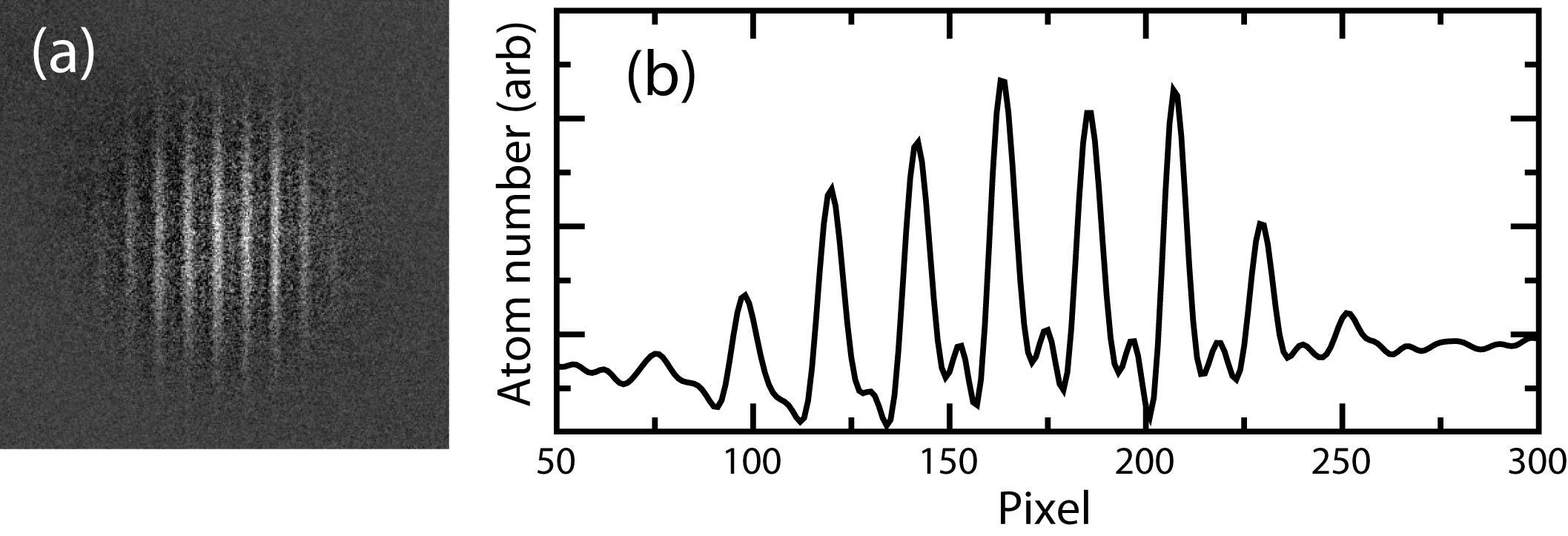
Figure 6: a) Image of atom cloud (after background subtraction) taken with several sidebands separated by 100 kHz imposed on one VSTPR beam. b) Cross sectional profile.

Instead of relying on an accurate pixel calibration, the splittings of the stripes can be determined by making $\omega_{1}=\omega_{2}+\delta_{12}$, where $\delta_{12}$ is a frequency shift imposed by an RF source. The resonant velocity classes are now determined by $2\mathbf{k}{\cdot}\mathbf{v}=({\Delta}m)\omega_{L}+\delta_{12}$. To demonstrate this idea, the retroreflecting mirror in Fig. 2 is replaced by a counterpropagating beam of the same diameter and power. This counterpropagating beam is derived from the original, so it is phase locked to $\omega_{1}$, but its frequency is shifted by two acousto-optic modulators (AOM) to achieve small $\delta_{12}~{}(<$1 MHz$)$. Additionally, we frequency modulate one AOM so that its instantaneous frequency is $\omega_{RF}$ + Asin($\omega_{m}t$), where $\omega_{RF}$ is the drive frequency, $\omega_{m}$ is the modulation frequency, and A is the maximum frequency deviation. This imparts frequency sidebands at $n\omega_{m}$, where $n$ is an integer, so that multiple $\delta_{12}$ are produced simultaneously. In Fig. 6, we show an image and cross section taken with $\omega_{m}=2{\pi}\times 100$ kHz. For $\delta_{12}=0$, the range of measurable Zeeman shifts is limited to the Doppler width of the atom cloud ($\simeq$1G). A nonzero $\delta_{12}$ overcomes this limitation by shifting the stripe to an accessible velocity class.

VII Conclusion

We have used velocity-selective resonances between magnetic sublevels of a single hyperfine level in ⁸⁵Rb to measure magnetic fields in a cold atom cloud. The resonances are easily observed with no additional laser frequencies than are required for MOTs, and can be used to measure magnetic fields with sub-mG resolution. Because of its simplicity, this technique should prove especially useful for aiding magnetic field compensation, for which purpose no calibration is required.

This work was funded by the Defense Advanced Research Projects Agency and the Office of Naval Research.

References

- Kasevich et al. (1991) M. Kasevich, D. S. Weiss, E. Riis, K. Moler, S. Kasapi, and S. Chu, Phys. Rev. Lett. 66, 2297 (1991).
- Boyer et al. (2004) V. Boyer, L. J. Lising, S. L. Rolston, and W. D. Phillips, Phys. Rev. A 70, 043405 (2004).
- McGuirk et al. (2002) J. M. McGuirk, G. T. Foster, J. B. Fixler, M. J. Snadden, and M. A. Kasevich, Phys. Rev. A 65, 033608 (2002).
- Chabé et al. (2007) J. Chabé, H. Lignier, P. Szriftgiser, and J. C. Garreau, Opt. Commun. 274, 254 (2007).
- Ringot et al. (2001) J. Ringot, P. Szriftgiser, and J. C. Garreau, Phys. Rev. A 65, 013403 (2001).
- Vuletić et al. (1998) V. Vuletić, C. Chin, A. J. Kerman, and S. Chu, Phys. Rev. Lett. 81, 5768 (1998).
- Isayama et al. (1999) T. Isayama, Y. Takahashi, N. Tanaka, K. Toyoda, K. Ishikawa, and T. Yabuzaki, Phys. Rev. A 59, 4836 (1999).
- Smith et al. (2003) G. A. Smith, S. Chaudhury, and P. S. Jessen, Journal of Optics B-Quantum and Semiclassical Optics 5, 323 (2003).
- Labeyrie et al. (2001) G. Labeyrie, C. Miniatura, and R. Kaiser, Phys. Rev. A 64, 033402 (2001).
- Alexandrov et al. (2004) E. B. Alexandrov, M. V. Balabas, A. K. Vershovski, and A. S. Pazgalev, Technical Physics 49, 779 (2004).
- Sheehy et al. (1990) B. Sheehy, S.-Q. Shang, P. van der Straten, S. Hatamian, and H. Metcalf, Phys. Rev. Lett. 64, 858 (1990).
- Hobbs (1997) P. C. D. Hobbs, Appl. Opt. 36, 903 (1997).