Radiative energy transfer in disordered photonic crystals

Abstract

The difficulty of description of the radiative transfer in disordered photonic crystals arises from the necessity to consider on the equal footing the wave scattering by periodic modulations of the dielectric function and by its random inhomogeneities. We resolve this difficulty by approaching this problem from the standpoint of the general multiple scattering theory in media with arbitrary regular profile of the dielectric function. We use the general asymptotic solution of the Bethe-Salpeter equation in order to show that for a sufficiently weak disorder the diffusion limit in disordered photonic crystals is presented by incoherent superpositions of the modes of the ideal structure with weights inversely proportional to the respective group velocities. The radiative transfer and the diffusion equations are derived as a relaxation of long-scale deviations from this limiting distribution. In particular, it is shown that in general the diffusion is anisotropic unless the crystal has sufficiently rich symmetry, say, the square lattice in 2D or the cubic lattice in 3D. In this case, the diffusion is isotropic and only in this case the effect of the disorder can be characterized by the single mean-free-path depending on frequency.

1 Introduction

The interest in structures with periodic modulations of the dielectric function (photonic crystals [1]) has been motivated initially by the possibility to modify substantially the spontaneous emission in such media. One of the main motives of the study, therefore, has been the existence of the complete band gap [2] when the propagation of light is completely inhibited inside some frequency region. Only relatively recently it has been realized that the periodicity of refractive index in photonic crystals by itself results in a number of unusual properties even in absence of the complete band gap [3, 4, 5, 6, 7, 8]. These properties do not necessarily require a strong contrast of the periodic modulation, i.e. the ratio of the minimum and the maximum values of the refractive index, and, particularly, can be observed even if the contrast is much weaker than needed for the gap to open. One of the illustrative examples is provided by dark modes [9, 10, 11], which are not coupled to plane waves propagating outside the structure. The existence of these modes is related to the point symmetry of the photonic crystal and, therefore, the dark modes present even if the contrast is very low. The dark modes, as well as other phenomena such as self-collimation and the negative refraction demonstrate that periodic spatial modulations of the dielectric function have more ways to affect the propagation of light than just producing a gap in the spectrum.

Real photonic crystal structures always contain one or another type of disorder regardless of a manufacturing procedure. It is crucially important, therefore, to understand to which extent disorder affects properties of these structures. This issue is of a great interest because an interplay between periodic and random variations of the refractive index creates new challenges for a theory of light propagation in inhomogeneous media, and promises new and unusual effects in the radiative transport.

The problem of the disorder in photonic crystals can be approached from two perspectives. On one hand, there is an issue of effects of disorder on spectral features of photonic crystals and their manifestation in such characteristics as reflection or transmission spectra. This research direction involves, for instance, studying such problems as a dependence of the width of the photonic band gap on the degree of the disorder [12, 13, 14]. A different type of questions arise when one is concerned with effects of disorder on propagation of light inside the photonic structure within the framework of the transport theory. Problems considered in this case include diffusion in the photonic crystals [15, 16] or enhanced backscattering [17, 18, 19].

The main objective of the current paper is to develop a general theoretical approach to wave transport in disordered photonic crystals, which would systematically, from first principles, take into account the periodic nature of the average refractive index. The microscopical nature of our approach distinguishes it from earlier papers, which relied either on ad hoc modifications of results obtained within the multiple scattering theory in statistically homogeneous media [19, 18], or on phenomenological assumptions regarding the distribution of the field in the bulk of the photonic crystal [16, 17]. For instance, it was assumed in the latter papers that propagation of light in the bulk of the photonic structure is the same as in statistically homogeneous random media, and the band structure of the photonic crystal only manifests itself within a narrow surface layer of the sample. This idea is obviously based on the assumption that multiple scattering destroys photonic modes of an ideal periodic structure so that the structure of the electromagnetic field in the bulk of the photonic crystal becomes indistinguishable from that of a regular disordered medium. A number of experimental and numerical results, however, cast doubts on this assumption. For instance, it was shown in [20] that photonic modes are completely developed in samples with linear dimensions as small as just a few periods. It was also determined experimentally that the mean-free-path, $\ell$, [see Eqs. (60) and (72)] due to disorder in real photonic crystals (see. e.g. Table I in [21]) substantially exceeds the lattice constant of the photonic crystal. Even for relatively high frequencies $\Omega a/2\pi c=1.6$ it was found that $\ell/a\approx 4$. Thus, even in this least favourable case there are about hundred elementary cells in a volume with the linear dimensions of the order of $\ell$. Comparing these two results and invoking ideas of the separation of length scales it is reasonable to expect that the underlying periodicity of the photonic crystals must still manifest itself even in the presence of disorder. In our paper we show that this expectation is indeed justified, and demonstrate explicitly the effects of periodicity on wave transport in the diffusive regime.

The standard multiple-scattering theory of wave transport in disordered media depends significantly on the plane-wave representation of the scattered field. The role of the plane waves is explicitly emphasized by the use of the Wigner function in derivations of the radiative energy transfer equations [22, 23, 24, 25]. In photonic crystals, however, approaches based on plane waves encounter significant difficulties because plane waves are not normal modes of the underlying ideal periodic structure. While the Wigner representation of the field-field correlation function itself remains, of course, valid even in such structures, the Wigner function, however, ceases to be a smooth function of coordinates, which is essential for the derivation of the radiative transfer and diffusion equations.

Qualitatively, one of the difficulties of the plane wave based approaches is due to the fact that the plane waves are scattered not only by the random fluctuations of the refractive index but also by its periodic modulation. The latter is a purely deterministic process and is responsible for the formation of photonic crystal modes, which can be considered as coherent superpositions of the plane waves. Thus, in order to describe wave transport in disordered photonic crystals one has to be able to separate the deterministic contribution to the scattering from the one caused by the disorder. This can be achieved by developing the transport theory on the base of photonic modes of an ideal crystal, but as we will see even within this approach the discrimination between coherent and incoherent processes is highly non-trivial. The second, more technical, difficulty in adapting the standard multiple scattering theory to photonic crystals arises from the fact that the theory developed for statistically uniform media heavily depends on certain assumptions (e.g. the translational invariance of the averaged Green’s function) that are not valid in disordered photonic crystals.

In the present paper we resolve these difficulties and develop a consistent multiple scattering theory of light transport in media with the periodic-on-average dielectric function. Some of the results obtained are actually valid also in media with arbitrary modulation of the background (average) dielectric functions. We introduce the interpretation of the field-field correlation function as the density matrix and show how it can be used to separate coherent and incoherent contributions in the transport. Using this idea we generalize the concept of specific intensities to the case of photonic crystals and derive respective radiative transfer equations. We also find an asymptotic solution of Bethe-Salpeter equation describing a steady state intensity distribution in an infinite media far away from sources, which we use to derive a diffusion equation in a steady state regime describing long scale spatial relaxation of the intensity toward the limiting distribution.

2 Multiple scattering in disordered photonic crystals

In the framework of the scalar model, the spatial distribution of the wave field at frequency $\omega$ in a disordered photonic crystal is governed by the Helmholtz equation

$$\Delta E_{\omega}(\bi{r})+\omega^{2}\widetilde{\epsilon}(\bi{r})E_{\omega}(\bi{r})=j(\bi{r}),$$ (1)

where $j(\bi{r})$ is the external source. Here and henceforth we use units with $c=1$. In (1) we have introduced the dielectric function

$$\widetilde{\epsilon}(\bi{r})=\epsilon(\bi{r})+\Delta\epsilon(\bi{r}),$$ (2)

which consists of two components. The periodic part, $\epsilon(\bi{r}+\bi{a})=\epsilon(\bi{r})$, constitutes the photonic crystal with $\bi{a}$ being the vector of lattice translations. The zero-mean random term, $\Delta\epsilon(\bi{r})$, describes the deviation of the dielectric function from the ideal periodic form. We assume that the random part of the refractive index is a zero-mean Gaussian random field, i.e. its statistical properties are completely characterized by the covariance $K(\bi{r}_{1},\bi{r}_{2})=\left\langle\Delta\epsilon(\bi{r}_{1})\Delta\epsilon(\bi{r}_{2})\right\rangle$. In A we provide a model of such inhomogeneities relevant for disordered photonic crystals. With this assumption (1) can be readily analyzed by standard diagrammatic techniques based on the Born series representation of the solutions of the integral (Lippmann-Schwinger) formulation of (1), which were developed in the theory of multiple wave scattering in statistically uniform media [26, 27, 28]. This approach is virtually model independent and can be applied for structures with arbitrary spatial profile of the deterministic part of the refractive index.

The Dyson equation for the Green’s function of (1) averaged over realizations of the disorder, $\bar{G}\equiv\left\langle G\right\rangle$, is obtained using the standard diagrammatic technique and has the form

$$\bar{G}_{\omega}(\bi{r},\bi{r}^{\prime})=G_{0}(\bi{r},\bi{r}^{\prime})+\int\rmd\bi{r}_{1}\rmd\bi{r}_{2}\,G_{0}(\bi{r},\bi{r}_{1})\Sigma_{\omega}(\bi{r}_{1},\bi{r}_{2})\bar{G}_{\omega}(\bi{r}_{2},\bi{r}^{\prime}),$$ (3)

where $\Sigma_{\omega}$ is the self-energy “defined” as a sum of all irreducible diagrams. We use somewhat cumbersome coordinate representation in order to emphasize its generality and independence of a particular form of the regular modulation $\epsilon(\bi{r})$. The latter determines the nonperturbed Green’s function, $G_{0}(\bi{r},\bi{r}^{\prime})$, which is assumed to be known. In particular, in disordered photonic crystals $G_{0}(\bi{r},\bi{r}^{\prime})$ is the Green’s function of the ideal periodic structure.

The main difference between statistically uniform media and disordered photonic crystals is reflected in this equation through symmetry properties of the unperturbed Green’s function. In periodic-on-average systems, this function is invariant with respect to lattice translations and the group of point symmetries of the underlying photonic structure, while in the uniform disordered systems it has full translational and rotational symmetry. In B we demonstrate that the averaged Green’s function and the self-energy posses the same translational and point symmetries as $G_{0}(\bi{r},\bi{r}^{\prime})$. We utilize these properties by expanding all related quantities in terms of photonic Bloch modes,

$$\Psi_{n,\bi{k}}(\bi{r})=\rme^{\rmi\bi{k}\cdot\bi{r}}u_{\bi{k},n}(\bi{r}),$$ (4)

where $u_{n,\bi{k}}(\bi{r})$ is periodic with the period of the photonic lattice, $\bi{k}$ is the Bloch wave vector lying inside the first Brillouin zone, and $n$ enumerates photonic bands. Using these functions we introduce the matrix representations of the quantities appearing in (3) according to

$$\eqalign{G_{0}(\bi{r}_{1},\bi{r}_{2})=&\sum_{\bi{k},n}g_{n}(\bi{k})\Psi_{\bi{k},n}(\bi{r}_{1})\Psi^{*}_{\bi{k},n}(\bi{r}_{2}),\cr\bar{G}_{\omega}(\bi{r}_{1},\bi{r}_{2})=&\sum_{\bi{k},n,m}G_{n,m}(\bi{k})\Psi_{\bi{k},n}(\bi{r}_{1})\Psi^{*}_{\bi{k},m}(\bi{r}_{2}),\cr\Sigma_{\omega}(\bi{r}_{1},\bi{r}_{2})=&\sum_{\bi{k},n,m}\Sigma_{n,m}(\bi{k})\epsilon(\bi{r}_{1})\Psi_{\bi{k},n}(\bi{r}_{1})\Psi^{*}_{\bi{k},m}(\bi{r}_{2})\epsilon(\bi{r}_{2}).}$$ (5)

The respective matrix elements in these expansions are

$$\eqalign{g_{n}(\bi{k})=\frac{1}{\omega^{2}-\omega_{n}^{2}(\bi{k})},\cr G_{n,m}(\bi{k})=\frac{1}{\mathcal{V}^{2}}\int_{\mathcal{V}}\rmd\bi{r}_{1}\,\rmd\bi{r}_{2}\,\epsilon(\bi{r}_{1})u^{*}_{\bi{k},n}(\bi{r}_{1})\bar{G}_{\omega}(\bi{r}_{1},\bi{r}_{2})u_{\bi{k},m}(\bi{r}_{2})\epsilon(\bi{r}_{2}),\cr\Sigma_{n,m}(\bi{k})=\frac{1}{\mathcal{V}^{2}}\int_{\mathcal{V}}\rmd\bi{r}_{1}\,\rmd\bi{r}_{2}\,u^{*}_{\bi{k},n}(\bi{r}_{1})\Sigma_{\omega}(\bi{r}_{1},\bi{r}_{2})u_{\bi{k},m}(\bi{r}_{2}),}$$ (6)

where $\omega_{n}^{2}(\bi{k})$ is the dispersion law of $n$-th band, the integration is performed over the elementary cell of the ideal structure, and $\mathcal{V}$ is the volume of the elementary cell. Deriving (6) we use the orthogonality condition of the Bloch functions

$$\int\rmd\bi{r}\,\epsilon(\bi{r})\Psi_{n,\bi{k}}^{*}(\bi{r})\Psi_{m,\bi{q}}(\bi{r})=\delta_{mn}\delta(\bi{k}-\bi{q}).$$ (7)

Using (6) we can rewrite (3) in the matrix form

$$G_{mn}(\bi{k})=g_{m}(\bi{k})\delta_{mn}+\sum_{l}g_{m}(\bi{k})\Sigma_{ml}(\bi{k})G_{ln}(\bi{k}).$$ (8)

This equation emphasizes the fact that the translational invariance of the self-energy prevents modes with different Bloch vectors to be mixed while states corresponding to the same Bloch vector but belonging to different bands are coupled by non-diagonal elements of the self-energy $\Sigma_{ml}(\bi{k})$.

In order to analyze the general effect of the disorder, we separate the diagonal, $\widehat{\Sigma}_{\mathrm{d}}(\bi{k})$, and the off-diagonal, $\widehat{\Sigma}_{\mathrm{o}}(\bi{k})$, parts of the self-energy representing the latter in the form

$$\widehat{\Sigma}(\bi{k})=\widehat{\Sigma}_{\mathrm{d}}(\bi{k})+\widehat{\Sigma}_{\mathrm{o}}(\bi{k}).$$ (9)

The diagonal part $\widehat{\Sigma}_{d}(\bi{k})$ modifies each band independently. It can be accounted for by introducing a modified Green’s function

$$\widetilde{G}_{0}(\bi{k})=\frac{1}{G_{0}^{-1}(\bi{k})-\widehat{\Sigma}_{\mathrm{d}}(\bi{k})},$$ (10)

which is determined by the Dyson equation similar to the one written for the standard case of a statistically homogeneous medium. In terms of the modified Green’s function (8) takes the form

$$\bar{G}=\widetilde{G}_{0}+\widetilde{G}_{0}\widehat{\Sigma}_{\mathrm{o}}\bar{G}.$$ (11)

Eqs. (10) and (11) show the two-fold role of the disorder in disordered photonic crystals. The disorder not only modifies each band separately similar to the case of the statistically homogeneous media, but also couples these modified bands. It is important to note that the band coupling is a subject of various selection rules. First, the most restrictive rule comes from the translational symmetry of the self-energy. As has been noted, it prevents states characterized by different Bloch vectors to be coupled. In other words, from the perspective of a band diagram one can have only “vertical” coupling. The second rule follows from the point symmetries. The self-energy transforms according to identity representation of the symmetry group of a given point in the reciprocal space of the photonic crystal. As a result, its matrix elements between states corresponding to different irreducible representations vanish. This selection rule has important implications for high-symmetry points and directions. In particular, it means that disorder does not lift the degeneracy at the points where the degenerate states are described by different or by multidimensional irreducible representations. The first can be shown by direct calculations of the respective matrix elements of the self-energy. The second follows from the following argument. The states corresponding to a representation with a dimension higher than $1$ can be coupled only with the states that transform according to the same presentation. As a result the modified state also transforms according to this presentation and, hence, the respective state should also be degenerate. This implies, in particular, that the degeneracy is not lifted at high-frequency $\Gamma$-points.

In order to analyze the effect of the band coupling in more details, we consider a two-band model when all bands but two (denoted by $1$ and $2$) remain uncoupled. The solution of the Dyson equation describing the coupled bands has the form

$$\bar{G}=\frac{1}{\mathcal{D}_{12}}\left(\begin{array}[]{cc}g_{2}^{-1}-\Sigma_{22}&\Sigma_{12}\\ \Sigma_{21}&g_{1}^{-1}-\Sigma_{11}\end{array}\right),$$ (12)

where $g_{i}$ and $\Sigma_{ij}$ are the respective matrix elements of the unperturbed Green’s function and the self-energy, respectively. The zeros of the function

$$\mathcal{D}_{12}=\left(g_{1}^{-1}-\Sigma_{11}\right)\left(g_{2}^{-1}-\Sigma_{22}\right)-\Sigma_{12}\Sigma_{21}$$ (13)

give the spectrum of averaged excitations. Introducing $\omega_{1,2}(\bi{k})$, the unperturbed dispersion laws of the interacting bands, the poles of averaged Green’s function can be written in the form

$$\bar{\omega}^{2}_{i}=\frac{1}{2}\left(\widetilde{\omega}_{1}^{2}+\widetilde{\omega}_{2}^{2}\right)\pm\frac{\Delta_{12}}{2}\sqrt{1+\eta_{12}}.$$ (14)

Here $\widetilde{\omega}_{1,2}^{2}=\omega_{1,2}^{2}-\Sigma_{11,22}$ are the band frequencies after the diagonal modification, $\Delta_{12}=\widetilde{\omega}_{1}^{2}-\widetilde{\omega}_{2}^{2}$, and

$$\eta_{12}=4\frac{\Sigma_{12}\Sigma_{21}}{\Delta_{12}^{2}}$$ (15)

is the parameter characterizing the strength of the band coupling. As one could expect, this parameter is proportional to the matrix elements of the self-energy between the coupled bands and is inversely proportional to the frequency separation of the modified bands. When this parameter is small, $\eta_{12}\ll 1$, the effect of the band coupling can be neglected and the photonic crystals can be described in a single band approximation. It should be noted, however, that in spite of formal similarity between the averaged Green’s function in the single band approximation and the respective expression for the uniform disordered medium, the transport properties of the two systems remain substantially different. The condition $\eta_{12}\ll 1$ can be easier satisfied at lower frequencies, when the band separation is of the order of magnitude of the fundamental band-gap. For higher frequency bands, however, the band coupling may play a significant role even in the case of photonic crystals with weak disorder and strong contrast of the refractive index.

3 Transport in disordered photonic crystals

3.1 General formalism

The transport properties of disordered media are characterized by the field-field correlation function

$$\rho_{\omega_{1},\omega_{2}}(\bi{r}_{1},\bi{r}_{2})=\left\langle E_{\omega_{1}}(\bi{r}_{1})E^{*}_{\omega_{2}}(\bi{r}_{2})\right\rangle,$$ (16)

which can be used to describe transfer of energy and, generally, spatial distributions and time evolutions of any quantity quadratic in the field. A relation between $\rho_{\omega_{1},\omega_{2}}(\bi{r}_{1},\bi{r}_{2})$ and the external sources is provided by the intensity propagator $\Pi(\bi{r}_{1},\bi{r}_{2};\bi{r}_{1}^{\prime}\bi{r}_{2}^{\prime})=\left\langle G_{\omega_{1}}(\bi{r}_{1},\bi{r}_{1}^{\prime})G_{\omega_{2}}^{*}(\bi{r}_{2},\bi{r}_{2}^{\prime})\right\rangle$ according to

$$\rho_{\omega_{1},\omega_{2}}(\bi{r}_{1},\bi{r}_{2})=\int\rmd\bi{r}_{1}^{\prime}\rmd\bi{r}_{2}^{\prime}\,\Pi(\bi{r}_{1},\bi{r}_{1}^{\prime};\bi{r}_{2},\bi{r}_{2}^{\prime})j_{\omega_{1}}(\bi{r}_{1}^{\prime})j^{*}_{\omega_{2}}(\bi{r}_{2}^{\prime}).$$ (17)

Using the standard diagrammatic technique one can show that the intensity propagator satisfies the Bethe-Salpeter equation, which can be written as

$$\eqalign{\Pi(\bi{r}_{1},\bi{r}_{2};\bi{r}_{1}^{\prime}\bi{r}_{2}^{\prime})={}&\bar{G}_{\omega_{1}}(\bi{r}_{1},\bi{r}_{1}^{\prime})\bar{G^{*}}_{\omega_{2}}(\bi{r}_{2},\bi{r}_{2}^{\prime})+\cr&\int\rmd\bi{r}_{3}\rmd\bi{r}_{3}^{\prime}\rmd\bi{r}_{4}\rmd\bi{r}_{4}^{\prime}\,\bar{G}_{\omega_{1}}(\bi{r}_{1},\bi{r}_{3})\bar{G^{*}}_{\omega_{2}}(\bi{r}_{2},\bi{r}_{4}){U}_{\omega_{1},\omega_{2}}(\bi{r}_{3},\bi{r}_{4};\bi{r}_{3}^{\prime},\bi{r}_{4}^{\prime})\cr&\qquad\qquad\times\Pi(\bi{r}_{3}^{\prime},\bi{r}_{4}^{\prime};\bi{r}_{1}^{\prime}\bi{r}_{2}^{\prime}).}$$ (18)

The kernel ${U}_{\omega_{1},\omega_{2}}$ is the irreducible vertex presented formally as a sum of irreducible diagrams [26]. We would like to emphasize that similarly to the Dyson equation, the Bethe-Salpeter equation holds for an arbitrary regular spatial modulation of the dielectric function, not necessarily periodic. We show in B that regardless of the spatial dependence of the regular part of the dielectric function, the irreducible vertex possesses an important property of reciprocity

$$U_{\omega_{1},\omega_{2}}(\bi{r}_{1},\bi{r}_{2};\bi{r}_{1}^{\prime},\bi{r}_{2}^{\prime})=U_{\omega_{1},\omega_{2}}(\bi{r}_{1}^{\prime},\bi{r}_{2}^{\prime};\bi{r}_{1},\bi{r}_{2}).$$ (19)

Additionally, in disordered photonic crystals this quantity is invariant with respect to lattice translations (see B) suggesting the following representation for the vortex

$$\eqalign{U_{\omega_{1},\omega_{2}}(\bi{r}_{1},\bi{r}_{2};\bi{r}_{1}^{\prime},\bi{r}_{2}^{\prime})={}&\sum_{v_{1,2},l_{1,2},\bi{q}_{i}}\epsilon(\bi{r}_{1})\epsilon(\bi{r}_{2})\epsilon(\bi{r}_{1}^{\prime})\epsilon(\bi{r}_{2}^{\prime})\cr&\qquad U^{v_{1},v_{2}}_{l_{1},l_{2}}(\bi{q}_{1},\bi{q}_{2};\bi{q}_{3},\bi{q}_{4})\delta\left(\overline{\bi{q}_{1}+\bi{q}_{4}-\bi{q}_{2}-\bi{q}_{3}}\right)\cr&\qquad\Psi_{\bi{q}_{1},v_{1}}(\bi{r}_{1})\Psi_{\bi{q}_{4},l_{2}}(\bi{r}_{2}^{\prime})\Psi^{*}_{\bi{q}_{2},v_{2}}(\bi{r}_{2})\Psi^{*}_{\bi{q}_{3},l_{1}}(\bi{r}_{1}^{\prime}),}$$ (20)

where the bar over a vector denotes the vector reduced to the first Brillouin zone.

Using Bethe-Salpeter equation, Eqs. (18) and (17) one can derive an equation for the field-field correlation function $\rho_{\omega_{1},\omega_{2}}(\bi{r}_{1},\bi{r}_{2})$. We present it in an integro-differential form, which is the most convenient for further analysis. To derive such an equation one can apply operators

$$\frac{1}{\epsilon(\bi{r}_{1,2})}\Delta_{1,2}+\omega^{2}_{1,2},$$ (21)

where indices $1$ and $2$ indicate a coordinate acted upon by the Laplacian, to both sides of (17). As a result, in the region of space free of external sources, one has

$$\eqalign{\left[\frac{1}{\epsilon(\bi{r}_{1})}\Delta_{1}-\frac{1}{\epsilon(\bi{r}_{2})}\Delta_{2}+\omega_{1}^{2}-\omega_{2}^{2}\right]&\rho_{\omega_{1},\omega_{2}}(\bi{r}_{1},\bi{r}_{2})=\cr&\int d\bi{r}_{1}^{\prime}d\bi{r}_{2}^{\prime}\,\mathcal{F}_{\omega_{1},\omega_{2}}(\bi{r}_{1},\bi{r}_{2};\bi{r}_{1}^{\prime},\bi{r}_{2}^{\prime})\rho_{\omega_{1},\omega_{2}}(\bi{r}_{1}^{\prime},\bi{r}_{2}^{\prime}),}$$ (22)

where

$$\eqalign{\mathcal{F}_{\omega_{1},\omega_{2}}(\bi{r}_{1},\bi{r}_{2};\bi{r}_{1}^{\prime},\bi{r}_{2}^{\prime})&=\frac{1}{\epsilon(\bi{r}_{1})}\Sigma_{\omega_{1}}(\bi{r}_{1},\bi{r}_{1}^{\prime})\delta(\bi{r}_{2}-\bi{r}_{2}^{\prime})-\frac{1}{\epsilon(\bi{r}_{2})}\Sigma_{\omega_{2}}^{*}(\bi{r}_{2},\bi{r}_{2}^{\prime})\delta(\bi{r}_{1}-\bi{r}_{1}^{\prime})\cr+&\int\rmd\bi{r}_{1}^{\prime\prime}\rmd\bi{r}_{2}^{\prime\prime}\left[\frac{\delta(\bi{r}_{1}-\bi{r}_{1}^{\prime\prime})}{\epsilon(\bi{r}_{1})}\bar{G}^{*}_{\omega_{2}}(\bi{r}_{2},\bi{r}_{2}^{\prime\prime})-\frac{\delta(\bi{r}_{2}-\bi{r}_{2}^{\prime\prime})}{\epsilon(\bi{r}_{2})}\bar{G}_{\omega_{1}}(\bi{r}_{1},\bi{r}_{1}^{\prime\prime})\right]\cr&\qquad\times U_{\omega_{1},\omega_{2}}(\bi{r}_{1}^{\prime\prime},\bi{r}_{2}^{\prime\prime};\bi{r}_{1}^{\prime},\bi{r}_{2}^{\prime}).}$$ (23)

This equation has been a subject of numerous investigations [26, 29], most of which were concerned with the radiative transfer or diffusion regimes in statistically homogeneous media. In many of those works, diffusion was understood as a transport process characterized by asymptotically slow (both in time and space) changes of the field intensity. In the spectral domain this behaviour manifests itself in the form of the characteristic “diffusion” pole of the intensity propagator, which is proportional to $\left(i\Omega-DQ^{2}\right)^{-1}$ in the limits $\Omega\rightarrow 0$, $Q\rightarrow 0$. Here frequency and wave vector transfers, $\Omega=\omega_{1}-\omega_{2}$ and $Q=q_{1}-q_{2}$, characterize slow spatiotemporal dynamics of intensity, and wave vectors $\bi q_{1}$ and $\bi q_{2}$ arise from the plane-wave representation of the scattered field. This reliance on the plane waves significantly complicates generalization of standard microscopic derivations of radiative transfer or diffusive equations to the case of disordered photonic crystals.

In order to better recognize the source of these difficulties and find a way to circumvent them, it is necessary to re-examine basic physical ideas about diffusion of light in disordered media. As a first step in this direction, in the current paper we consider time independent spatial distribution of the wave intensity in an infinite medium far away from the sources. This regime arises in the case of a monochromatic source, when the field in the structure harmonically depends on time, $\propto\exp(-i\omega t)$, so that $\Omega=0$. In this case, the equation for the field-field correlation function $\rho=\left\langle E_{\omega}E^{*}_{\omega}\right\rangle$ (hereafter we omit the lower index corresponding to frequency) can be obtained from (22) by setting $\omega_{1}=\omega_{2}=\omega$:

$$\left[\frac{1}{\epsilon(\bi{r}_{1})}\Delta_{1}-\frac{1}{\epsilon(\bi{r}_{2})}\Delta_{2}\right]\rho(\bi{r}_{1},\bi{r}_{2})=\int\rmd\bi{r}_{1}^{\prime}\rmd\bi{r}_{2}^{\prime}\,\mathcal{F}(\bi{r}_{1},\bi{r}_{2};\bi{r}_{1}^{\prime},\bi{r}_{2}^{\prime})\rho(\bi{r}_{1}^{\prime},\bi{r}_{2}^{\prime}),$$ (24)

where $\mathcal{F}\equiv\mathcal{F}_{\omega,\omega}$. Using (24), the optical theorem (the Ward identity) can be derived [26] in the form $\mathcal{F}(\bi{r},\bi{r};\bi{r}_{1}^{\prime},\bi{r}_{2}^{\prime})\equiv 0$, which is especially useful from the technical point of view. Integrating this equation over $\bi{r}$ we obtain the Ward identity in the form

$$\Sigma(\bi{r}_{2},\bi{r}_{1})-\Sigma^{*}(\bi{r}_{1},\bi{r}_{2})=\int\rmd\bi{r}_{1}^{\prime\prime}\rmd\bi{r}_{2}^{\prime\prime}\left[\bar{G}(\bi{r}_{2}^{\prime\prime},\bi{r}_{1}^{\prime\prime})-\bar{G}^{*}(\bi{r}_{1}^{\prime\prime},\bi{r}_{2}^{\prime\prime})\right]U(\bi{r}_{1}^{\prime\prime},\bi{r}_{2}^{\prime\prime};\bi{r}_{1},\bi{r}_{2}).$$ (25)

The physical picture of the transport in disordered media is developed using close relation of the function $\rho(\bi{r}_{1},\bi{r}_{2})$ to both transport characteristics and coherence properties of the field. The description of transport (e. g. the energy density and the flux) is based on the property that the averaged values of any quantity quadratic in field can be expressed in terms of convolution of respective operators with $\rho(\bi{r}_{1},\bi{r}_{2})$ [see Eqs. (33) and (39) below]. The coherence properties are described considering $\rho(\bi{r}_{1},\bi{r}_{2})$ as the coherence function [30, 31].

A quantity, which simultaneously describes such transport related characteristics as energy density and flux and coherence properties of the system, is well known in quantum statistics. It is called the density matrix [32]. Indeed, on the one hand, the density matrix can be used to calculate current and energy densities, and on the other hand, the density matrix describes mixed states, which can be characterized as incoherent superpositions of pure or coherent states. Using the density matrix analogy one can think of the field-field correlation function as a characteristic of such a mixed state of the wave field in disordered media. Separation of coherent and incoherent properties of the field would then involve finding states whose incoherent superposition would reproduce the field at the level of function $\rho(\bi{r}_{1},\bi{r}_{2})$. However, before developing this idea any further, we need to demonstrate that the field-field correlation function has indeed all the formal properties of the density matrix.

We expand $\rho(\bi{r}_{1},\bi{r}_{2})$ in terms of the eigenstates of the nonperturbed system, say, the modes of the ideal photonic crystal, writing

$$\rho(\bi{r}_{1},\bi{r}_{2})=\sum_{\mu,\nu}\rho_{\mu,\nu}\Psi_{\mu}(\bi{r}_{1})\Psi_{\nu}^{*}(\bi{r}_{2}),$$ (26)

where summation over indices $\mu$ and $\nu$ enumerating the eigenstates can involve integration. It is easy to see from the definition of the correlation function that coefficients $\rho_{\mu,\nu}$ constitute a Hermitian matrix. This matrix can be diagonalized, which corresponds to the spectral representation of the statistical operator in quantum mechanics, by means of a unitary transformation to another basis

$$\bar{\Psi}_{\bar{\kappa}}=B_{\bar{\kappa}\mu}\Psi_{\mu}$$ (27)

so that one has (Mercer’s theorem [30, 33])

$$\rho(\bi{r}_{1},\bi{r}_{2})=\sum_{\bar{\kappa}}\rho_{\bar{\kappa}}\bar{\Psi}_{\bar{\kappa}}(\bi{r}_{1})\bar{\Psi}^{*}_{\bar{\kappa}}(\bi{r}_{2})$$ (28)

with $\rho_{\bar{\kappa}}\geq 0$, which follows from the fact that $\rho(\bi{r}_{1},\bi{r}_{2})$ is non-negatively defined [34]. The diagonal representation of the correlation function can be interpreted as an incoherent superposition or mixture of pure or coherent states $\bar{\Psi}_{\bar{\kappa}}$, which, in turn, as follows from (27) are coherent superpositions of the states $\Psi_{\mu}$. In order to clarify the exact meaning of this expression let us show that the correlation function can be used to calculate the energy density of the field and its Poynting vector in much the same way as the density matrix is used in quantum statistics.

The energy density of the field in a steady state can be presented as

$$w(\bi{r})=\frac{1}{2}\left[\omega^{2}\widetilde{\epsilon}(\bi{r})|E(\bi{r})|^{2}+|\nabla E(\bi{r})|^{2}\right],$$ (29)

where $\widetilde{\epsilon}(\bi{r})$ is the total dielectric function including both regular and the random components. By introducing the operator

$$\widehat{w}=-(\nabla_{1}-\nabla_{2})^{2}/4,$$ (30)

one can show that the averaged energy density can be expressed in terms of the function

$$w(\bi{r}_{1},\bi{r}_{2})=\widehat{w}\rho(\bi{r}_{1},\bi{r}_{2})$$ (31)

as

$$\left\langle w(\bi{R})\right\rangle=w(\bi{R},\bi{R}),$$ (32)

where we used the Helmholtz equation to arrive at (32). One can see that this equation can be presented in the typical for quantum statistics form as

$$\left\langle w(\bi{R})\right\rangle=\mathrm{Tr}\left[\widehat{\rho}\,\widehat{w}{R}\right],$$ (33)

where $\widehat{w}{R}=\delta(\bi{r}_{1}-\bi{R})\delta(\bi{r}_{2}-\bi{R})\widehat{w}$.

As an example let us consider the case when the density matrix has the form of an incoherent superposition of the eigenstates $\Psi_{\mu}$ of the ideal system. Then from (33) we find

$$\left\langle w(\bi{R})\right\rangle=\sum_{\mu}\rho_{\mu}w_{\mu}(\bi{R}),$$ (34)

where we have introduced the energy density of the $\mu$-th mode

$$w_{\mu}(\bi{R})=\widehat{w}\left.\Psi_{\mu}(\bi{r}_{1})\Psi_{\mu}^{*}(\bi{r}_{2})\right|_{\bi{r}_{1}=\bi{r}_{2}=\bi{R}}.$$ (35)

This expression provides a clear explanation of the notion of incoherent superposition. Indeed, the average energy of the field in this expression is presented as a sum of energies of individual modes $\Psi_{\mu}(\bi{r})$ as it is expected for the addition of incoherent fields as oppose to the sum of the field amplitudes expected for the coherent fields.

Similar expressions can be obtained for the average value of the Poynting vector, $\bi{S}=\rmi\omega\left[E^{*}\nabla E-E\nabla E^{*}\right]/2$, which can be calculated using the operator

$$\widehat{\bi{S}}=-\frac{\rmi\omega}{2}\left(\nabla_{1}-\nabla_{2}\right),$$ (36)

which gives

$$\left\langle\bi{S}(\bi{R})\right\rangle=\bi{S}(\bi{R},\bi{R}),$$ (37)

where

$$\bi{S}(\bi{r}_{1},\bi{r}_{2})=\widehat{\bi{S}}\rho(\bi{r}_{1},\bi{r}_{2}).$$ (38)

In the case when the density matrix is diagonal in the basis of the eigenfunctions of the ideal system we see again that the average Poynting vector is a sum of Poynting vectors of each mode, which indicates the absence of any interference effects in the superposition of modes $\Psi_{\mu}(\bi{r})$:

$$\left\langle\bi{S}(\bi{R})\right\rangle=\mathrm{Tr}\left[\widehat{\rho}\,\widehat{\bi{S}}{R}\right]=\sum_{\mu}\rho_{\mu}\bi{S}_{\mu}(\bi{R}),$$ (39)

where $\widehat{\bi{S}}{R}=\delta(\bi{r}_{1}-\bi{R})\delta(\bi{r}_{2}-\bi{R})\widehat{\bi{S}}$ and $\bi{S}_{\mu}(\bi{R})$ is the distribution of the Poynting vector in the $\mu$-th mode

$$\bi{S}_{\mu}(\bi{R})=\widehat{\bi{S}}\left.\Psi_{\mu}(\bi{r}_{1})\Psi_{\mu}^{*}(\bi{r}_{2})\right|_{\bi{r}_{1}=\bi{r}_{2}=\bi{R}}.$$ (40)

It is seen from Eqs. (34) and (39) that $\rho_{\mu}$ have the meaning of the weights of the incoherent superposition. More generally, if we normalize $\rho(\bi{r}_{1},\bi{r}_{2})$ in such a way that $\mathrm{Tr}[\widehat{\rho}]\equiv 1$, we can interpret $\rho_{\bar{\kappa}}$, the eigenvalues of the matrix $\rho_{\mu,\nu}$, as the distribution function in the space of the states $\bar{\Psi}_{\bar{\kappa}}$. The values of any quantity, quadratic in field averaged over the disorder realizations, therefore, can be calculated as the average over the distribution function $\rho_{\bar{\kappa}}$ in the similar way as it is done in quantum mechanics. We would like to emphasize here that the emergence of the incoherent superposition in the problem of wave propagation is directly related to averaging over realizations of disorder. Without averaging the density matrix defined in (28) would have a form $\rho_{\mu,\nu}\propto a_{\mu}a_{\nu}$, and matrices of such form have a single non-zero eigenvalue. As a result, the sums in (34) and (39) would consist of just one term indicating that $\rho$ represents a pure or coherent state.

The notion of incoherent superposition expressed by Eqs. (34) and (39) also allows one to provide a physical meaning for the states $\bar{\Psi}_{\bar{\kappa}}$ diagonalizing the density matrix. The spatial field distribution in a random media can be in principle presented as a linear combination of functions from any full system: plane waves, Bloch waves, etc. The concept of normal modes as well defined spatial distributions of the fields that can be excited separately one from another is not very useful here. Indeed the distribution of the field in a random media is so complex that at any given frequency it is impossible to excite a single mode out of infinitely many degenerate modes. In this situation, functions $\bar{\Psi}_{\bar{\kappa}}$ play a special role as such distributions of the field whose linear combination is purely incoherent in the sense of Eqs. (34) and (39). The form of these functions is determined by remaining coherence effects in the scattered waves, and thus, by using the density matrix formalism we achieve a separation between coherent and incoherent contributions to the energy transport in disordered systems. In other words, one can say that the functions diagonalizing the density matrix describe the modes, which provide the energy transfer.

In order to illustrate these general idea, let us consider a case of wave scattering in a homogeneous random medium. In the case, of an infinite medium and asymptotically far away from the sources the field-field correlation function restores its translational invariance: $\rho(\bi{r}_{1},\bi{r}_{2})\rightarrow\rho(\bi{r}_{1}-\bi{r}_{2})$. Using plane waves as a basis we can rewrite (26) for this particular case as

$$\rho(\bi{r}_{1},\bi{r}_{2})=\int\rmd\bi{q}\rmd\bi{k}\,\rho_{\mathrm{un}}(\bi{k})\delta(\bi{k}-\bi{q}).$$ (41)

One can see that the density matrix in this case is diagonal in the basis of the plane waves so that they are responsible for the incoherent transport.

3.2 The field-field correlation in an infinite photonic crystal: asymptotic behaviour

In this subsection we consider a solution of the steady-state Bethe-Salpeter equation (24) for the correlation function $\rho(\bi{r}_{1},\bi{r}_{2})$ valid in an infinite photonic crystal asymptotically far away from the sources. Besides providing an important non-trivial example of the application of our formalism, this solution shows how the periodicity of the underlying photonic structure affects asymptote of the intensity distribution in the disordered structure and provides a starting point for deriving the diffusion equation. Using Eqs. (19) and (25) one can check that (24) is solved by

$$\rho^{(\infty)}(\bi{r}_{1},\bi{r}_{2})=\frac{1}{2\,\rmi N}\left[\bar{G}^{*}(\bi{r}_{2},\bi{r}_{1})-\bar{G}(\bi{r}_{1},\bi{r}_{2})\right],$$ (42)

where $N$ is a normalization constant independent of coordinates. Using the reciprocity theorem [26] this is rewritten as

$$\rho^{(\infty)}(\bi{r}_{1},\bi{r}_{2})=-\mathrm{Im}\left[\bar{G}(\bi{r}_{1},\bi{r}_{2})\right]/N.$$ (43)

This solution is valid in a general case regardless of the specific form of the regular modulation of the dielectric function and the distribution of the disorder. In the case of statistically uniform media it is reduced to a form found in Refs. [35] and [36]. Thus we can consider this function as the asymptotic distribution of the field-field correlator, which can be called for this reason an equilibrium density matrix.

In the case of disordered photonic crystals, function $\rho^{(\infty)}(\bi{r}_{1},\bi{r}_{2})$ can be expanded in terms of normal modes of the underlying periodic structure. According to (5) we can present this expansion in the following form

$$\rho^{(\infty)}(\bi{r}_{1},\bi{r}_{2})=\sum_{\bi{k},n,m}\rho^{(\infty)}_{m,n}(\bi{k})\Psi_{\bi{k},n}(\bi{r}_{1})\Psi^{*}_{\bi{k},m}(\bi{r}_{2}),$$ (44)

where

$$\eqalign{\rho^{(\infty)}_{m,n}(\bi{k})&=\left[\bar{G}_{n,m}^{*}(\bi{k})-\bar{G}_{m,n}(\bi{k})\right]/2\,\rmi N\cr&=\frac{1}{N\mathcal{V}^{2}}\int_{\mathcal{V}}\rmd\bi{r}_{1}\,\rmd\bi{r}_{2}\,\epsilon(\bi{r}_{1})u^{*}_{\bi{k},n}(\bi{r}_{1})\mathrm{Im}\,\bar{G}_{\omega}(\bi{r}_{1},\bi{r}_{2})u_{\bi{k},m}(\bi{r}_{2})\epsilon(\bi{r}_{2}).}$$ (45)

This expression shows that in the basis of normal modes of an ideal periodic structure, the density matrix is diagonal with respect to the quasi-wave vector $\bi{k}$, but is not diagonal with respect to the band indices. Following Eqs. (26), (27), and (28) we diagonalized the matrix $\rho^{(\infty)}_{m,n}(\bi{k})$ by a unitary transformation

$$\bar{\Psi}_{\bi{k},\bar{m}}=\sum_{n}B_{\bar{m}n}(\bi{k})\Psi_{\bi{k},n}.$$ (46)

Since the diagonalization procedure involves only band indices and leaves the Bloch vector intact, functions $\bar{\Psi}_{\bi{k},\bar{m}}(\bi{r})$ can also be presented in the Bloch form similar to (4)

$$\bar{\Psi}_{\bi{k},\bar{m}}(\bi{r})=\rme^{\rmi\bi{k}\cdot\bi{r}}\bar{u}_{\bi{k},\bar{m}}(\bi{r}).$$ (47)

Transformation (46) preserves the scalar product because of unitarity so that

$$\int\rmd\bi{r}\,\epsilon(\bi{r})\bar{\Psi}_{\bi{k},\bar{m}}^{*}(\bi{r})\bar{\Psi}_{\bi{q},\bar{n}}(\bi{r})=\delta(\bi{k}-\bi{q})\delta_{\bar{n}\bar{m}}.$$ (48)

Using this property we normalize $\rho^{(\infty)}$ defining

$$N=-\pi\int_{\mathcal{V}}\rmd\bi{r}\,\epsilon(\bi{r})\mathrm{Im}\,[\bar{G}(\bi{r},\bi{r})],$$ (49)

where the integration is performed over the elementary cell of the ideal structure. Equations (42) and (49) define $\rho^{(\infty)}$ as the asymptotic form of density matrix, which according to Eqs. (44) and (46) is an incoherent superposition of the states $\bar{\Psi}_{\bi{k},\bar{m}}$ with respective weights.

As was discussed, the eigenvalues of $\rho^{(\infty)}$ define the probability distribution function on the space of the states $\bar{\Psi}_{\bi{k},\bar{m}}(\bi{r})$ parametrized by the number of band $\bar{m}$ and by the point in the first Brillouin zone $\bi{k}$. As follows from the Dyson equation the singularities of the averaged Green’s function and, respectively, of the eigenvalues of $\rho^{(\infty)}_{m,n}$ are determined by the dispersion law of the average excitations [see e.g. (13)]. For more detailed analysis we consider the situation when we can neglect the band coupling so that the averaged Green’s function is given by (10). In this case, the eigenvalues of the density matrix as functions of the quasi-wave vector have the largest values, when $\bi{k}$ obeys the dispersion equation for a given frequency. In other words, these eigenvalues reach maximum values on equifrequency surfaces, $F_{m}(\omega)$, corresponding to different bands of the ideal photonic crystal. The width of these maxima is proportional to $\mathrm{Im}[{\Sigma_{d}}_{m}(\bi{k})]$ [see (9)]. If the disorder is weak in the sense of the Ioffe-Regel criterion (see below), then for frequencies, which do not lie at band edges, we can obtain

$$\rho^{(\infty)}(\bi{r}_{1},\bi{r}_{2})\approx\frac{\pi}{2N\omega}\sum_{m}\int_{F_{m}(\omega)}\rmd\bi{k}\,\frac{1}{|v_{m}(\bi{k})|}\rme^{-|\boldsymbol{\gamma}_{m}(\bi{k})\cdot(\bi{r}_{1}-\bi{r}_{2})|}\Psi_{\bi{k},m}(\bi{r}_{1})\Psi^{*}_{\bi{k},m}(\bi{r}_{2}),$$ (50)

where the integration runs along the equifrequency surfaces, $\bi{v}_{m}(\bi{k})=\nabla{k}\omega_{m}(\bi{k})$ is the group velocity, and

$$\boldsymbol{\gamma}_{m}(\bi{k})=-\frac{\mathrm{Im}[{\Sigma_{\mathrm{d}}}_{m}(\bi{k})]\bi{v}_{m}(\bi{k})}{2\,\omega\,v_{m}^{2}(\bi{k})}=\frac{1}{2}\ell_{m}^{-1}(\bi{k})\widehat{\bi{v}}_{m}(\bi{k}).$$ (51)

Here $\widehat{\bi{v}}_{m}(\bi{k})$ is the unit vector along the direction of the group velocity and we have expressed the imaginary part of the self-energy in terms of the respective mean-free-path $\ell_{m}(\bi{k})$, which is defined later in (60).

As follows from (50) in the limit of vanishing disorder, which corresponds to the on-shell approximation [26, 29, 37, 38, 39] in the standard theory of transport in statistically homogeneous media, the density matrix takes the universal limit

$$\rho^{(\infty)}_{0}(\bi{r}_{1},\bi{r}_{2})=\frac{\pi}{2N\omega}\sum_{m}\int_{F_{m}(\omega)}\rmd\bi{k}\,\frac{1}{v_{m}(\bi{k})}\Psi_{\bi{k},m}(\bi{r}_{1})\Psi^{*}_{\bi{k},m}(\bi{r}_{2}).$$ (52)

The magnitude of the group velocity is, in general, not constant along the equifrequency surfaces. As a result, different states are not equally presented in the equilibrium distribution, as is seen from Eqs. (50) and (52). In particular, if there are flat bands [40] with low group velocity near the frequency $\omega$, then these bands would give the main contribution to $\rho^{(\infty)}_{0}$. Another example of a highly inhomogeneous distribution is provided by the frequencies when an equifrequency surface touches the boundary of the Brillouin zone. In this case, the magnitude of the group velocity becomes very low at the points of contact resulting in an increased weight of the respective states in the equilibrium distribution (see Figure 1).

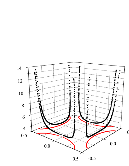
Figure 1: (Colour online) The dependence of $1/v_{m}(\bi{k})$ along the equifrequency surface corresponding to $\omega a/2\pi=0.41$. The horizontal plane is the first Brillouin zone. Here and below the calculations are presented for a square lattice 2D PC made of dielectric cylinders with the contrast of the refractive indices $n=2$ and with the radius-period ratio $r/a=0.4$.

It should be noted that the on-shell approximation is poorly suited for studying the correlation properties of the field. Indeed, the function $\rho^{(\infty)}_{0}(\bi{r}_{1},\bi{r}_{2})$ does not tend to any limit as $|\bi{r}_{1}-\bi{r}_{2}|\to\infty$ while $\rho^{(\infty)}(\bi{r}_{1},\bi{r}_{2})$ in (50) obviously vanishes in this limit. Thus, for this purpose one has to use (42) or in the case of a weak disorder the simpler version (50), as it has been practically done in [36], where additionally the approximation of spherical equifrequency surfaces was used.

However, for studying transport properties the on-shell approximation may by appropriate because, as follows from Eqs. (32) and (37), the energy density and the Poynting vector are determined by the behaviour of $\rho(\bi{r}_{1},\bi{r}_{2})$ near the diagonal $\bi{r}_{1}=\bi{r}_{2}$. We estimate the effect of the exponential term in (50) by calculating the average energy density. The density matrix in the on-shell approximation yields the energy density as a sum of contributions of different modes [see (34)]

$$\left\langle w(\bi{R})\right\rangle=\sum_{\bi{k},m}\rho^{(\infty)}_{\bi{k},m}w_{\bi{k},m}(\bi{R}),$$ (53)

where $w_{\bi{k},m}(\bi{R})$ is the energy density of the mode $\Psi_{\bi{k},m}$ of the ideal photonic crystal. The exponential term in (50) can be shown to modify each contribution by the factor

$$\sim 1-\frac{1}{\left[4\omega\ell_{m}(\bi{k})\right]^{2}}.$$ (54)

In order to evaluate the correction, we note that $\omega\ell_{m}(\bi{k})$ is a parameter of the Ioffe-Regel type [27], which is expected to be much larger than unity far from the localization regime, so that the deviation of the equilibrium density matrix from (52) can be neglected in the analysis of transport quantities.

The problem of special interest is what happens in an immediate vicinity of the complete band gap. Formal application of (60) gives vanishing mean-free-path for the modes lying at the edge of the gap. This means that approximation (50) for the density matrix is no longer valid and that the modes of the ideal photonic crystal are not a good approximation for the modes $\bar{\Psi}_{\bar{\mu}}$. Such nonperturbative reconstruction of the modes constitutes a special problem and is not considered in the present paper. Therefore, in what follows we restrict to the frequencies which are not too close to the complete gap so that the condition $\omega\ell_{m}(\bi{k})>1$ can always be fulfilled if the magnitude of the inhomogeneities is not too high.

Let us conclude the analysis of the equilibrium distribution by outlining two significant differences between the transport in statistically homogeneous media and disordered photonic crystals. The most essential difference is that the radiative transport in photonic crystals is provided not by plane waves but by the modes, which reflect properties of the ideal structure. Indeed, these are the modes of the photonic crystals that constitute $\rho^{(\infty)}(\bi{r}_{1},\bi{r}_{2})$ rather than pure plane waves. As a result, even in the asymptotic distribution of the energy density the disorder does not wash out the features specific for the ideal structure. In the case of weak disorder when the energy density can be approximated by (53), one can see explicitly that frequencies near the fundamental gap and higher, the spatial profile of $w_{\bi{k},m}(\bi{R})$ is highly inhomogeneous on the length scale of the elementary cell [41]. This inhomogeneity is stable, to some extent, with respect to averaging over the equilibrium distribution function. Most clearly this effect should be seen for frequencies near the lower edge of the fundamental gap. Indeed, as follows from the variational principle [1] at such frequencies the field distribution takes higher values in the regions with higher values of the refractive index for each point on the equifrequency surface. The same obviously holds for the energy density of each mode. Thus, we can conclude that even the long scale asymptotic behaviour of intensity in disordered photonic crystals is highly inhomogeneous. This property is unexpected from the point of view of the transport in statistically homogeneous media, where the distinctive feature of this limit is the homogeneous distribution of the energy density [42]

The second important feature of the field distribution in photonic crystals is its significant anisotropy as a function of direction of the Bloch vector. Anisotropy itself is not, of course, the specific feature of disordered photonic crystals. The similar effect can be expected in regular anisotropic media, where the group velocity depends on the direction of the wave vector. In disordered photonic crystals, however, this anisotropy can be very pronounced, especially near the frequencies corresponding to the edges of (partial) band gaps.

3.3 The radiative transfer equation

Applying (37) to the equilibrium state described in the previous subsection,

$$\bi{S}^{(\infty)}(\bi{r}_{1},\bi{r}_{2})=\widehat{\bi{S}}\rho^{(\infty)}(\bi{r}_{1},\bi{r}_{2}),$$ (55)

and using the symmetry properties of the equilibrium distribution given as $\rho^{(\infty)}(\bi{r}_{1},\bi{r}_{2})=\rho^{(\infty)}(\bi{r}_{2},\bi{r}_{1})$, we can immediately see that the flux in this state vanishes: $\bi{S}^{(\infty)}(\bi{R},\bi{R})=0$. This is of course a result expected for an asymptotic regime in the infinite medium. In order to describe states with a non-zero flux, which are most relevant to experimental situations, we have to consider the correlation function at a finite distance from the sources or in a finite-sized medium. In this case, we cannot expect that the same modes $\bar{\Psi}$ will diagonalized the correlation function, but if the deviations from the equilibrium state are small we can assume that non-diagonal elements decay very fast when one moves away from the main diagonal of the density matrix. Then, instead of trying to find the true diagonalizing states we will follow the same approach as in the standard transport theory in statistically homogeneous medium and convert the non-diagonal density-matrix into a slowly changing in the real space function. The field-field correlator in this representation takes the form of

$$\rho(\bi{r}_{1},\bi{r}_{2})=\sum_{\bi{k},\bar{m}}\mathcal{I}_{\bi{k},\bar{m}}(\bi{R})\bar{\Psi}_{\bi{k},\bar{m}}(\bi{r}_{1})\bar{\Psi}_{\bi{k},\bar{m}}^{*}(\bi{r}_{2}),$$ (56)

where $\bi{R}=(\bi{r}_{1}+\bi{r}_{2})/2$ and $\mathcal{I}_{\bi{k},\bar{m}}(\bi{R})$ are smooth functions of the coordinate $\bi{R}$. The functions $\mathcal{I}_{\bi{k},\bar{m}}(\bi{R})$ can be interpreted as specific intensities of the respective modes $\bar{\Psi}_{\bi{k},\bar{m}}$. In order to show it let us calculate the average energy density and the average Poynting vector. Using representation (56) in Eqs. (32) and (37) we obtain

$$\eqalign{\left\langle w(\bi{R})\right\rangle=\sum_{\bi{k},\bar{m}}\mathcal{I}_{\bi{k},\bar{m}}(\bi{R})w_{\bi{k},\bar{m}}(\bi{R}),\cr\left\langle\bi{S}(\bi{R})\right\rangle=\sum_{\bi{k},\bar{m}}\mathcal{I}_{\bi{k},\bar{m}}(\bi{R})\bi{S}_{\bi{k},\bar{m}}(\bi{R}),}$$ (57)

where we have used Eqs. (35) and (40) to define formally the energy density, $w_{\bi{k},\bar{m}}$ and the Poynting vector, $\bi{S}_{\bi{k},\bar{m}}$, corresponding to the states $\bar{\Psi}_{\bi{k},\bar{m}}$. Equations (57) agree with the intuitive concept of the specific intensity justifying our identification for functions $\mathcal{I}_{\bi{k},\bar{m}}$.

In order to derive an equation for the specific intensities, we calculate the matrix element of both sides of (24) between the states $\bar{\Psi}^{*}_{\bi{k}+\bi{q}/2,\bar{n}}$ and $\bar{\Psi}_{\bi{k}-\bi{q}/2,\bar{n}}$ and then use the assumption of smooth $\mathcal{I}_{\bi{k},\bar{m}}(\bi{R})$ as expressed by (91). Calculations based on the separation of length scales (see details in C) lead to the radiative transfer equation in the form

$$\omega\,{\bi{V}}_{\bar{m}}(\bi{k})\cdot\nabla_{\bi{R}}\mathcal{I}_{\bi{k},\bar{m}}(\bi{R})=\mathrm{Im}[\Sigma_{\bar{m},\bar{m}}(\bi{k})]\mathcal{I}_{\bi{k},\bar{m}}(\bi{R})+\int\rmd\bi{q}\,\sum_{\bar{n}}\sigma_{\bar{m},\bar{n}}(\bi{k},\bi{q})\mathcal{I}_{\bi{q},\bar{n}}(\bi{R}).$$ (58)

Here and below the matrix elements for the self-energy and the irreducible vertex in the basis provided by the states $\bar{\Psi}_{\bar{\mu}}$ are related to the matrix elements defined in Eqs. (6) and (20) through transformation (46).

In equation (58) we have introduced several important quantities. The velocity ${\bi{V}}_{\bar{m}}(\bi{k})$ determines the direction of the “ray” corresponding to the mode $\bar{\Psi}_{\bi{k},\bar{m}}$ and is expressed in terms of the group velocity of the photonic crystal modes as

$$\bi{V}_{\bar{m}}(\bi{k})=\frac{1}{\omega}\sum_{n}\left|B_{\bar{m},n}(\bi{k})\right|^{2}\omega_{n}(\bi{k})\bi{v}_{n}(\bi{k}).$$ (59)

The spatial decay of the initial distribution $\mathcal{I}_{\bi{k},m}(\bi{R})$ concentrated in a single mode towards equilibrium is quantified by the mean-free-path

$$\ell_{\bar{m}}^{-1}(\bi{k})=-\frac{\mathrm{Im}[\Sigma_{\bar{m},\bar{m}}(\bi{k})]}{\omega V_{\bar{m}}(\bi{k})}.$$ (60)

As follows from the optical theorem, the decay is a result of the redistribution of energy between the modes specified by different points in the first Brillouin zone and different band numbers. Making use of representation (20) the scattering kernel, which describes the redistribution, can be shown to have the form

$$\sigma_{\bar{m},\bar{n}}(\bi{k},\bi{q})=N\rho^{(\infty)}_{\bar{m}}(\bi{k})U^{\bar{m},\bar{m}}_{\bar{n},\bar{n}}(\bi{k},\bi{k},\bi{q},\bi{q}).$$ (61)

Initially, in relatively small samples or near the boundary of a big sample, the distribution of energy can be arbitrary complex. For example, almost all energy can be concentrated in only few modes. The distribution changes along the sample according to (58) and eventually $\mathcal{I}_{\bi{k},\bar{m}}(\bi{R})$ tends to $\rho^{(\infty)}_{\bi{k},\bar{m}}$, which cancels both sides of (58). This confirms our interpretation of $\rho^{(\infty)}_{\bi{k},\bar{m}}$ as the asymptotic equilibrium distribution.

If we can neglect the interband coupling and use the on-shell approximation, which is justifiable in the limit of weak and short-scale disorder, the picture significantly simplifies since in this approximation $B_{\bar{m},n}(\bi{k})$ become just identity matrices and the density matrix can be approximated by (52). This means that the transport is provided by the modes of the ideal photonic crystal corresponding to the frequency $\omega$ and the specific intensity $\mathcal{I}_{\bi{k},\bar{m}}$ has the transparent meaning of the intensity of these modes. The spatial distribution of the specific intensity is governed by the same equation (58) with the velocity $\bi{V}_{\bar{m}}(\bi{k})$ substituted by the respective group velocity $\bi{V}_{\bar{m}}(\bi{k})\to\bi{v}_{m}(\bi{k})$ as follows from (59).

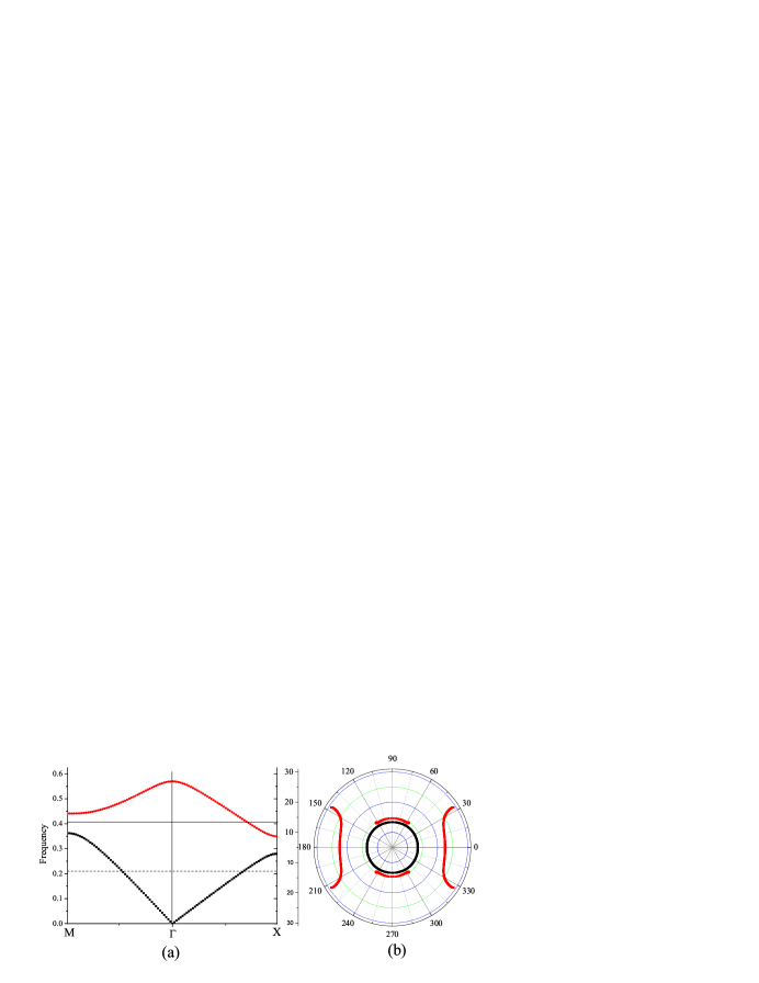
Figure 2: (Colour online) (a) The band structure of the ideal photonic crystal with the same parameters as in Figure 1. Only two bands used in calculations for Figs. 1, 2b and 3 are shown. The horizontal lines correspond to the frequencies $\omega a/2\pi=0.21$ and $0.41$. (b) The scattering amplitude $\sigma(\bi{k},\bi{q})/\omega^{3}V^{2}$ between the states belonging to the first ($\omega a/2\pi=0.21$, the internal points) and the second ($\omega a/2\pi=0.41$, the points corresponding to higher values) bands as a function of the angle between the vectors $\bi{k}$ and $\bi{q}$. The direction of the initial Bloch wave vector $\bi{q}$ is taken along the $\Gamma X$ direction for both frequencies, thus the angle in (b) is counted from the $\Gamma X$ direction.

In order to illustrate the specific features of the radiative transfer equation in disordered photonic crystals, we calculate the scattering kernel $\sigma_{\bar{m},\bar{n}}(\bi{k},\bi{q})$ for a 2D structure made of dielectric discs in the limit of weak disorder. We approximate the intensity propagator by the sum of the ladder diagrams and additionally assume the $\delta$-correlated disorder when $K(\bi{r}_{1},\bi{r}_{2})=V^{2}\delta(\bi{r}_{1}-\bi{r}_{S})\delta(\bi{r}_{1}-\bi{r}_{2})$, where $\bi{r}_{S}$ denotes points lying in a thin shell near the surface of the ideal disc [see A]. In this case the specific intensity is concentrated at the equifrequency surfaces $F_{m}(\omega)$ so that it can be presented as $\mathcal{I}_{\bi{k},m}(\bi{R})=\widetilde{\mathcal{I}}_{\bi{k},m}(\bi{R})\delta\left[\omega^{2}-\omega_{m}^{2}(\bi{k})\right]$. The amplitudes $\widetilde{\mathcal{I}}_{\bi{k},m}(\bi{R})$ satisfy the radiative transfer equation of the same structure as (58) with the scattering amplitude between the states on the equifrequency surface given by

$${\sigma}_{m,n}(\bi{k},\bi{q})=\frac{\omega^{3}V^{2}}{v_{n}(\bi{q})\mathcal{V}^{2}}\int_{S}\rmd\bi{r}\,|u_{\bi{k},m}(\bi{r})|^{2}|u_{\bi{q},n}(\bi{r})|^{2},$$ (62)

where the integration is performed in a thin shell near the surface of the ideal disc. We show the dependence of $\sigma_{m,n}(\bi{k},\bi{q})$ on the direction of the final Bloch wave vector in Figure 2b for two cases when the frequency $\omega$ is well below the frequency of the fundamental gap $\omega_{G}$ ($\omega_{G}\approx 0.28$ for the structure used in the numerical calculations) and when $\omega\gtrsim\omega_{G}$. As one can see, for low frequencies the scattering amplitude is close to isotropic (the variation of the scattering amplitude is not visible in this scale), which is the consequence of slow spatial variation of the Bloch amplitudes $u_{\bi{k},m}(\bi{r})$ and the shape of the equifrequency surface close to spherical. However, when $\omega$ approaches $\omega_{G}$ both the spatial variation of the Bloch amplitudes and the shape of the equifrequency surface become nontrivial resulting in strongly anisotropic scattering. The interesting feature of this dependence is that the scattering rates between the states, which belong to the same band (the points corresponding to $\omega a/2\pi=0.41$ near the horizontal line), are noticeably higher than the scattering amplitudes connecting the states in the different bands (points near the vertical axis). It should be noted that since the gap is not complete the scattering amplitude remains finite for all directions.

The expression for the mean-free-path $\ell_{m}(\bi{k})$ in terms of the scattering amplitude $\sigma_{m,n}(\bi{k},\bi{q})$ is found from the requirement for $\rho^{(\infty)}$ to solve the radiative transfer equation,

$$\ell^{-1}_{m}(\bi{k})=\frac{1}{\omega v_{m}(\bi{k})}\sum_{n}\int\rmd\bi{q}\,\sigma_{m,n}(\bi{k},\bi{q}),$$ (63)

where the integral runs over the respective equifrequency surfaces. Substituting (62) into this expression we find $\ell^{-1}_{m}(\bi{k})$ in terms of the Bloch amplitudes. The same result can be obtained from (60) using for the self-energy the same approximation as for deriving (62).

The evaluation of the mean-free-path for the same frequencies as in Figure 2 is presented in Figure 3. It is seen that for the relatively low frequencies the mean-free-path only weakly depends on the direction of the Bloch wave vector thus reproducing the well-known results for statistically homogeneous media. In a vicinity of the partial band gap the anisotropic scattering manifests in strong directional dependence of the mean-free-path. This is especially evident for an intermediate frequency $\omega a/2\pi=0.31$, for which near the $\Gamma M$-direction the mean-free-path drops by the factor of $5$.

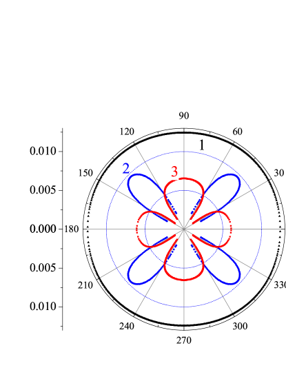
Figure 3: (Colour online) The directional dependence of the mean-free-path $\ell(\omega)\omega^{4}/V^{2}$ for frequencies $\omega a/2\pi=0.21$ (curve $1$), $0.31$ (curve $2$) and $0.41$ (curve $3$). The angle is counted from the $\Gamma X$-direction.

3.4 The diffusion equation

The right-hand side of (58) describing spatial variations of the specific intensities consists of the sum of two terms. In order to appreciate their physical significance let assume that at small distances from the source only single mode is excited so that the specific intensity can be presented in the following form

$$\mathcal{I}_{\bi{k},m}\propto\mathcal{I}(R)\delta_{m,m_{0}}\delta(\bi{k}-\bi{k}_{0}).$$ (64)

The first of the right hand terms in (58) describes exponential spatial decay of this specific intensity due to scattering and redistribution of the energy among other modes. At small distances this term dominates and solution of (58) can be presented in the same form as (64) with exponential spatial dependence. However, at distances from the source exceeding the mean-free-path this term diminishes and the second, integral term, starts determining the spatial distribution of the specific intensities, which is no longer exponential. One can describe this situation at asymptotically large distances taking into account that in this limit the density matrix $\rho(\bi{r}_{1},\bi{r}_{2})$ must be close to its limiting value $\rho^{(\infty)}(\bi{r}_{1},\bi{r}_{2})$ so that one can present $\rho(\bi{r}_{1},\bi{r}_{2})$ using an appropriate expansion near $\rho^{(\infty)}_{\bi{k},m}$. Drawing an analogy with the derivation of the diffusion approximation in the standard case [29, 42, 27] and assuming that the photonic crystal has the centre of symmetry we present specific intensities in the following form

$$\mathcal{I}_{\bi{k},m}(\bi{R})=\frac{1}{v_{m}(\bi{k})}\left[W^{-1}w_{\mathrm{d}}(\bi{R})+\widehat{\bi{v}}_{m}(\bi{k})\mathsf{T}^{-1}\bi{S}_{\mathrm{d}}(\bi{R})\right],$$ (65)

where $w_{\mathrm{d}}(\bi{R})$ and $\bi{S}_{\mathrm{d}}(\bi{R})$ are assumed to be slowly changing functions of $\bi{R}$, while $W$ and $\mathsf{T}$ are scalar and tensor respectively, which do not depend on spatial coordinates. With an appropriate choice of these quantities one can show that $w_{\mathrm{d}}(\bi{R})$ and $\bi{S}_{\mathrm{d}}(\bi{R})$ in (65) can be presented as

$$\eqalign{w_{\mathrm{d}}(\bi{R})=\frac{1}{\mathcal{V}}\int_{\mathcal{V}(\bi{R})}\rmd\bi{r}\,w(\bi{r},\bi{r}),\cr\bi{S}_{\mathrm{d}}(\bi{R})=\frac{1}{\mathcal{V}}\int_{\mathcal{V}(\bi{R})}\rmd\bi{r}\,\bi{S}(\bi{r},\bi{r}),}$$ (66)

where the integration is performed over the elementary cell with the coordinate $\bi{R}$; $w(\bi{r}_{1},\bi{r}_{2})$, and $\bi{S}(\bi{r}_{1},\bi{r}_{2})$ are defined by Eqs. (31) and (38), respectively. These expressions clarify the physical meaning of $w_{d}(\bi{R})$ and $\bi{S}_{d}(\bi{R})$ as long scale envelopes of the averaged energy density and the flux, respectively. $W$ and $\mathsf{T}$ in (65) are found to be

$$W=\frac{\omega}{2}\lambda(\omega),\qquad\mathsf{T}=\frac{\omega}{2}\sum_{m}\int\rmd\bi{k}\,\widehat{\bi{v}}_{m}(\bi{k})\otimes\widehat{\bi{v}}_{m}(\bi{k}).$$ (67)

where $\otimes$ denotes the tensor product, $(\bi{v}\otimes\bi{u})_{ij}=v_{i}u_{j}$ and $\lambda(\omega)$ is the density of states of the photonic crystal defined as $\lambda(\omega)=\sum_{\mu}\delta(\omega-\omega_{\mu})$.

The equations with respect to $w_{\mathrm{d}}(\bi{R})$ and $\bi{S}_{\mathrm{d}}(\bi{R})$ can be derived from the radiative transfer equation. Summation over all states on the respective equifrequency surface yields the energy conservation law

$$\nabla\cdot\bi{S}_{\mathrm{d}}(\bi{R})=0.$$ (68)

Multiplying both sides of (58) by $\widehat{\bi{v}}_{m}(\bi{k})$ and summing over all states we obtain

$$\nabla\mathsf{D}\nabla w_{\mathrm{d}}(\bi{R})=0,$$ (69)

where the diffusion tensor $\mathsf{D}(\omega)$ up to a constant factor is defined by $\mathsf{D}(\omega)=\mathsf{T}\mathsf{M}^{-1}\mathsf{T}$ with the current relaxation kernel [43]

$$\mathsf{M}=\frac{\omega^{2}\lambda(\omega)}{4}\sum_{m}\int d\bi{k}\,\left[\ell^{-1}_{m}(\bi{k})-\sum_{n}\int\rmd\bi{q}\,\frac{\sigma_{mn}(\bi{k},\bi{q})}{\omega v_{m}(\bi{k})}\widehat{\bi{v}}_{m}(\bi{k})\otimes\widehat{\bi{v}}_{n}(\bi{q})\right].$$ (70)

It is important to note that despite the scalar character of the initial Helmholtz equation (1) the diffusion in photonic crystals is characterized by a diffusion tensor rather than by a single diffusion constant. In particular, if the periodic modulation is characterized by a rectangular (noncubic) elementary cell then the eigenvalues of the tensor corresponding to different principal directions will be different resulting in anisotropic diffusion.

This diffusion anisotropy, however, appears only in low symmetry photonic crystals. If the point symmetry group of a particular structure is such that irreducible representations of the full rotation group remain irreducible for the point group of the crystal, the diffusion tensor is reduced to a scalar form. Indeed, crystals with such symmetries, e.g. crystals with square and hexagonal lattices in 2D and cubic and fcc lattices in 3D, do not allow non-trivial tensors of the second rank [44] In this case the diffusion, despite of the strong directional dependence of the scattering kernel $\sigma_{mn}(\bi{k},\bi{q})$, is isotropic and is characterized by the diffusion constant

$$D=\frac{F(\omega)}{d\lambda(\omega)}\,\frac{\ell(\omega)}{1-\left\langle\cos(\theta)\right\rangle},$$ (71)

where $d$ is the dimensionality of the problem, $F(\omega)=\sum_{m}\int d\bi{k}\,1$ is the total area of the equifrequency surface,

$$\ell^{-1}(\omega)=\frac{1}{F(\omega)}\sum_{m}\int\rmd\bi{k}\,\ell_{m}^{-1}(\bi{k})$$ (72)

and

$$\left\langle\cos(\theta)\right\rangle\equiv\frac{\ell(\omega)}{F(\omega)}\sum_{m,n}\int\rmd\bi{k}\rmd\bi{q}\,\frac{\sigma_{mn}(\bi{k},\bi{q})}{\omega v_{m}(\bi{k})}\,\widehat{\bi{v}}_{m}(\bi{k})\cdot\widehat{\bi{v}}_{n}(\bi{q}).$$ (73)

The expression for the diffusion coefficient has the same general structure as for statistically homogeneous media [29] with the transport velocity $v_{E}(\omega)=F(\omega)/\lambda(\omega)$ and the “transport mean-free-path” $\ell(\omega)/(1-\left\langle\cos\theta\right\rangle)$. The transport velocity is independent on the details of the disorder distribution owing to the $\delta$-functional approximation for the correlation function $K(\bi{r}_{1},\bi{r}_{2})$, which is valid if the frequencies corresponding to morphological resonances at the typical inhomogeneity size is much higher than the range of frequencies under consideration [45, 46, 47]. Figure 4 shows the frequency dependence of $\ell(\omega)$ for a disordered photonic crystal with the square lattice. It should be noted that the minimum of $\ell(\omega)$ is reached at the band edge in the $\Gamma X$-direction (see Figure 2a) and is due to the significant drop of the group velocity when the equifrequency surface touches the boundary of the first Brillouin zone.

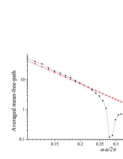
Figure 4: (Colour online) The dependence of the effective mean-free-path $\ell(\omega)/V^{2}$ (dashed line, squares) on frequency in log-log scale. The solid line (circles) shows the dependence $\propto\omega^{3}$ (this asymptotics for low frequencies is due to the dimensionality of the problem).

It should be emphasized, however, that the possibility to introduce a single scalar diffusion constant and, respectively, to describe transport by a single transport mean-free-path is not a a result of the disorder destroying the effect of periodicity but rather is the consequence of the underlying symmetry of the photonic crystal. In the case of low symmetry structures the diffusion is described by a tensor, and is characterized by different effective mean-free-paths for different principle directions of the diffusion tensor.

4 Conclusion

In this paper we developed a systematic approach based on multiple scattering analysis to the theoretical description of incoherent transport properties of disordered photonic crystals in the steady state regime. The main difficulty in developing such a theory using a standard plane-wave based multiple scattering approach lies in the separation between waves scattering due to periodic modulations of the dielectric constant and scattering due to random deviations from the periodicity. One might think that this difficulty is readily resolved by incorporating modes of the ideal photonic crystal instead of plane waves into the standard transport theory. However, such a straightforward approach fails because of the inherent presence of two spatial scales, the period of the crystal and the main-free-path, both of which has to be retained in the theory. As a result, a formally constructed Wigner distribution, which is the main technical tool in deriving the radiative transfer equation in the regular case of statistically homogeneous medium, loses its smooth spatial dependence and, hence, its methodological usefulness.

We showed that these difficulties can be overcome if one incorporates the concept of the radiative transfer as a incoherent process into the foundation of the theory. In order to achieve this, we showed that the field-field correlation function, $\rho(\bi{r}_{1},\bi{r}_{2})=\left\langle E(\bi{r}_{1})E^{*}(\bi{r}_{2})\right\rangle$, has all the properties of a density matrix defined in quantum statistics, and hence, can be interpreted as such. This interpretation allowed us to separate coherent and incoherent contributions to the transport and eventually obtain radiative transfer and diffusion equations for media with periodically modulated average dielectric function.

We found an exact asymptotic solution, $\rho^{(\infty)}$, of the Bethe-Salpeter equation (42), which describes the limiting form of the correlation function in an infinite medium asymptotically far away from the sources. This function determines the asymptotic distribution of the intensity of the field, which was shown to be highly spatially non-uniform and anisotropic. This result should be contrasted with the case of statistically homogeneous medium, in which the asymptotic distribution of intensity is spatially uniform. It is important that the properties of the intensity distribution even inside an infinite photonic crystal are determined by the normal modes of the underlying periodic structure. This result casts serious doubts on the assumption made in Refs. [15, 16] that the field distributions deep inside a photonic crystal and a statistically homogeneous media do not differ from each other, and that the anisotropy of the light emerging from photonic crystals is formed within a narrow layer at the boundary.

The asymptotic character of $\rho^{(\infty)}$ is expressed by the absence of flux in this state. Using analogy with the statistical physics we can interpret $\rho^{(\infty)}$ as an equilibrium distribution. In order to describe actual energy transfer, one needs to consider small deviations from equilibrium. We derived generalized forms of radiative transfer and diffusion equations valid for disordered photonic crystals and obtained general expressions for the scattering cross-section, mean free path, and the diffusion coefficient. As an example, we calculated the cross-section for one particular model of a photonic crystal and demonstrated how the underlying periodic structure effects disorder induced scattering of photonic modes. In particular, we found that the scattering cross-section describing the redistribution of the energy between modes becomes highly anisotropic at high frequencies. The mean-free-path of a particular mode, which describes the rate of redistributing the correspondent specific intensity, also depends strongly on the direction of the respective Bloch vector. The numerical calculations show that for a chosen frequency near the (partial) band gap the mean-free-path may vary almost by the order of magnitude. Such significant variation presents especial interest from the perspective of the problem of the Anderson localization.

The interesting feature of the transport in the disordered photonic crystals is that even if scattering between different modes may be highly anisotropic it does not necessarily imply an anisotropic diffusion. Indeed, if the point symmetry of the crystal is sufficiently rich, e.g. in 2D this is rotational symmetry of the third order or higher, then all tensors of the second rank describing the intrinsic macroscopic properties are proportional to the unit tensor. That is the diffusion is necessarily isotropic and is characterized by a single diffusion constant. The mean-free-path appears in this constant averaged over the respective equifrequency surface.

The derivation of the transport equations can be generalized to describe the radiative transport in more general situations than considered in the paper. Principally, the equilibrium distribution given by $\rho^{(\infty)}$ holds in the presence of the boundary as well. The latter is accounted through the boundary conditions determining Green’s functions. However, whether the respective density matrix can be described near the boundary as a long-scale perturbation of $\rho^{(\infty)}$ or not presents a special interesting problem.

Finally, we would like to comment on the possibility to extend the consideration provided in the paper to a non-steady-state regime. By a direct analogy with the standard case, a slow dynamics in the diffusion regime can be accounted for by assuming $w_{d}$ in (65) to be time dependent. However, a rigourous theory, which would yield this limit is yet to be developed. From the perspectives of the presented consideration, the main formal obstacle is the fact that $\rho_{\omega_{1},\omega_{2}}$ is generally not non-negatively defined if $\omega_{1}\neq\omega_{2}$. This problem, of course, exists and is recognized in the standard theory of multiple scattering in homogeneous media as well. In order to ensure positivity of the specific intensities, it was suggested to consider a coarse-grained Wigner distribution [48]. A possibility to generalize our approach to time-dependent correlation functions and their possible relation with the density matrix formalism is an open problem.

Appendix A A model of Gaussian inhomogeneities in photonic crystals

A Gaussian random field $\Delta\epsilon(\bi{r})$ can be defined in two equivalent ways. The functional definition is based on the requirement of an integral

$$I_{f}=\int\rmd\bi{r}\,f(\bi{r})\Delta\epsilon(\bi{r})$$ (74)

to be a Gaussian random variable for an arbitrary function $f(\bi{r})$. The statistical definition states that a multi-point correlation function of a zero-mean Gaussian field is expressed in terms of the two-point correlation function

$$\left\langle\Delta\epsilon(\bi{r}_{1})\ldots\Delta\epsilon(\bi{r}_{2n})\right\rangle=\sum_{\mathrm{pairs}}K(\bi{r}_{\alpha},\bi{r}_{\beta})\ldots K(\bi{r}_{\gamma},\bi{r}_{\delta}),$$ (75)

where the summation is taken over all possible pairings of the points $\bi{r}_{1},\ldots,\bi{r}_{2n}$ and $K(\bi{r}_{1},\bi{r}_{2})=\left\langle\Delta\epsilon(\bi{r}_{1})\Delta\epsilon(\bi{r}_{2})\right\rangle$.

Property of integral (74) being a Gaussian random variable is consistent with the intuitive idea about a Gaussian random field, while property (75) is convenient from the technical point of view for developing the perturbation theory [26]. Both these properties, however, might seem somewhat artificial from the perspective of disordered photonic crystal. Here we would like to present a simple model of the disorder in a photonic crystal that naturally results in simulation of the inhomogeneities by a Gaussian random field.

Let the ideal structure be constituted by spheres with the dielectric constant $\epsilon_{1}$ at the sites of a periodic lattice. Furthermore, we assume that the disorder in this system is constituted by slight variations of the size of the spheres, while their positions are fixed. Thus, we can represent the spatial modulation of the dielectric function in the disordered crystal in the form

$$\widetilde{\epsilon}(\bi{r})=\epsilon_{0}+\sum_{\bi{R}}\delta\epsilon_{\bi{R}}(\bi{r}+\bi{R}),$$ (76)

where $\bi{R}$ are the lattice vectors, $\epsilon_{0}$ is the background dielectric constant, and $\delta\epsilon_{\bi{R}}(\bi{r}+\bi{R})$ is the deviation from the background value in the elementary cell with the coordinate $\bi{R}$. By the construction $\delta\epsilon_{\bi{R}}(\bi{r})=\epsilon_{1}-\epsilon_{0}$ inside the sphere and it equals to $0$ elsewhere. We represent the spatial distribution of the dielectric function in the form adapted in (1), i.e. $\widetilde{\epsilon}(\bi{r})=\epsilon(\bi{r})+\Delta\epsilon(\bi{r})$, where $\epsilon(\bi{r})$ describes the distribution in the ideal structure and

$$\Delta\epsilon(\bi{r})=\sum_{\bi{R}}\left(\delta\epsilon_{\bi{R}}(\bi{r}+\bi{R})-\delta\epsilon_{0}(\bi{r}+\bi{R})\right)$$ (77)

with $\delta\epsilon_{0}(\bi{r})$ being the deviation from the background value in the ideal structure.

Clearly $\Delta\epsilon(\bi{r})$ is not zero in shells near the boundaries of the spheres constituting the ideal structure. It is positive in the spheres with the radius larger than the radius of the ideal spheres and is negative in smaller spheres. We simulate this function by presenting it in the form

$$\Delta\epsilon(\bi{r})=\sum_{\bi{R}}\Delta\epsilon_{\bi{R}}u(\bi{r}+\bi{R}),$$ (78)

where $u(\bi{r})$ is a non-random function different from zero in a thin shell near the boundary of the ideal sphere and the random amplitudes $\Delta\epsilon_{\bi{R}}$ have the Gaussian distribution with zero mean value and are independent in different elementary cells. Using (78) in the integral in (74) one has a Gaussian random variable and, hence, $\Delta\epsilon(\bi{r})$ is the Gaussian random field.

This model, obviously, can be generalized by allowing the random variables $\Delta\epsilon_{\bi{R}}$ to be a (usual) Gaussian random field rather than a constant inside each elementary cell. Such model of the disorder would account not only for the size dispersion of the spheres but also for the roughness of their surfaces. Assuming that $\Delta\epsilon{r}$ in different elementary cells are not correlated we obtain

$$K(\bi{r}_{1},\bi{r}_{2})=\left\langle\Delta\epsilon_{\bi{r}_{1}}\Delta\epsilon_{\bi{r}_{2}}\right\rangle u(\bi{r}_{1})u(\bi{r}_{2})$$ (79)

if $\bi{r}_{1}$ and $\bi{r}_{2}$ are situated inside the same elementary cell and $K(\bi{r}_{1},\bi{r}_{2})=0$ otherwise. For calculations in the main text we have used the simplest model of spheres with uniform sizes and with centers at the sites of an ideal lattice but with rough surfaces. Thus we take $u(\bi{r})=1$ in a thin shell around the ideal sphere (respectively, the circle in 2D) and

$$\left\langle\Delta\epsilon_{\bi{r}_{1}}\Delta\epsilon_{\bi{r}_{2}}\right\rangle=V^{2}\delta(\bi{r}_{1}-\bi{r}_{2}).$$ (80)

Appendix B Symmetries of the averaged Green’s function, the self-energy and the irreducible vertex

Leaving the problem of convergence of the perturbational series aside, the symmetry properties of the averaged Green’s function $\left\langle G(\bi{r}_{1},\bi{r}_{2})\right\rangle$, the self-energy $\Sigma(\bi{r}_{1},\bi{r}_{2})$, and the irreducible vertex $U(\bi{r}_{1},\bi{r}_{2};\bi{r}^{\prime}_{1},\bi{r}^{\prime}_{2})$ can be proven on the diagram by diagram basis [26]. We demonstrate the typical line of arguments by proving that if the correlation function of inhomogeneities is invariant with respect to lattice translations then so is the averaged Green’s function.

Any diagram in the perturbational expansion of $\left\langle G(\bi{r}_{1},\bi{r}_{2})\right\rangle$ has the form of a line with $2n$ internal ($n\geq 0$) and $2$ terminating vertices. The internal vertices divide the line on $2n+1$ segments, which are the graphical representations of the non-perturbed Green’s function of the ideal structure. The internal vertices are connected pair-wise by the lines of the correlation function.

Clearly the value of a diagram with fixed values of the coordinates corresponding to the vertices does not change if we shift the coordinates of all points (internal and terminating) by the vector of the lattice translation. Indeed, the Green’s function lines and the lines corresponding to the correlation functions do not change because of the translational invariance of these functions. Furthermore, we note that in order to obtain the contribution of the diagram into $\left\langle G(\bi{r}_{1},\bi{r}_{2})\right\rangle$ we need to integrate with respect to coordinates of the internal vertices. Finally, we observe that the uniform shift of the coordinates of all vertices produces the diagram, which corresponds to the perturbational series for $\left\langle G(\bi{r}_{1}+\bi{R},\bi{r}_{2}+\bi{R})\right\rangle$.

This line of arguments proves the translational invariance of the averaged Green’s function, the self-energy and the irreducible vertex. In order to prove the reciprocity of the Green’s function and the self-energy

$$\left\langle G(\bi{r}_{1},\bi{r}_{2})\right\rangle=\left\langle G(\bi{r}_{2},\bi{r}_{1})\right\rangle,\qquad\Sigma(\bi{r}_{1},\bi{r}_{2})=\Sigma(\bi{r}_{2},\bi{r}_{1}),$$ (81)

we need the version of the arguments sketched above, which includes the directionality of the lines constituting the diagram. The reciprocity would follow then from invariance of the diagram with respect to the reversion of the directionality of all lines. For the irreducible vertex we additionally need to take into account that the correlation function connecting upper and lower lines is mapped to itself upon the reverting. Thus, we have

$$U(\bi{r}_{1},\bi{r}_{2};\bi{r}^{\prime}_{1},\bi{r}^{\prime}_{2})=U(\bi{r}^{\prime}_{1},\bi{r}^{\prime}_{2};\bi{r}_{1},\bi{r}_{2}).$$ (82)

We complete the consideration of the symmetry properties by proving the invariance of the self-energy with respect to the point symmetries of the photonic crystal. More specifically, we show that if the correlation function transforms according to the identity representation of the respective group, then so does the self-energy. The proof is based on the property of the unperturbed Green’s function $G_{0}(\bi{r}_{1},\bi{r}_{2})$ to transform according to the identity representation

$$\mathtt{T}\,G_{0}(\bi{r}_{1},\bi{r}_{2})\equiv G_{0}(\mathtt{T}^{-1}\,\bi{r}_{1},\mathtt{T}^{-1}\,\bi{r}_{2})=G_{0}(\bi{r}_{1},\bi{r}_{2}),$$ (83)

where $\mathtt{T}$ is an element of the point symmetry group. The proof of the invariance of the self-energy uses the same arguments as above with the only difference that now instead of shift or inversion operators we act with $\mathtt{T}$ on all points of the diagram.

It follows from this consideration that the eigenfunctions of the Dyson equation can be classified according to the irreducible representations of the group of the point symmetries of the ideal structure. We use this fact in the paper when we discuss the effect of the disorder on the degenerate points in the spectrum of the photonic crystal.

Appendix C Separation of spatial scales in close-to-equilibrium regimes

The main assumption used for the derivation of the radiative transfer equation and the diffusion equation in the paper is that the spatial scales of variation of the specific intensity or the envelope of the energy density and of the functions describing the modes of the ideal photonic crystal can be separated. Physically this assumption implies that the slowly varying functions do not lead to coupling between different Bloch modes. As a result, one can neglect the smooth functions while calculating the respective scalar products.

In order to give a formal expression for the separation of length scales we consider a photonic crystal mode $\Psi_{\bi{k},m}(\bi{r})$ modulated by a smooth function $f(\bi{r})$

$$h_{\bi{k},m}(\bi{r})=f(\bi{r})\Psi_{\bi{k},m}(\bi{r}).$$ (84)

The smoothness of the function $f(\bi{r})$ can be quantified by $\left\langle\bi{p}\right\rangle_{f}$ and $\left\langle p^{2}\right\rangle_{f}$, where

$$\left\langle\bi{p}\right\rangle_{f}=\int\rmd\bi{p}\,\bi{p}f({\bi{p}})$$ (85)

and $f({\bi{p}})$ is the Fourier image of $f(\bi{r})$. The limit of smooth $f(\bi{r})$ can, thereby, be formalized as $\left\langle\bi{p}\right\rangle_{f}\to 0$ and $\left\langle p^{2}\right\rangle_{f}\to 0$. In this limit the weighted scalar product of $h_{\bi{k},m}(\bi{r})$ with the mode $\Psi_{\bi{q},n}(\bi{r})$ is written as

$$\left(\Psi_{\bi{q},n},h_{\bi{k},m}\right)\equiv\int\rmd\bi{r}\,\epsilon(\bi{r})\Psi^{*}_{\bi{q},n}(\bi{r})h_{\bi{k},m}(\bi{r})=f({\bi{k}-\bi{q}})\mathcal{U}_{n,m}(\bi{q},\bi{k}),$$ (86)

where

$$\mathcal{U}_{n,m}(\bi{q},\bi{k})=\int_{\mathcal{V}}\rmd\bi{r}\,\epsilon(\bi{r})u^{*}_{\bi{q},n}(\bi{r})u_{\bi{k},m}(\bi{r}).$$ (87)

The inverse Fourier transform of (86) with respect to $\bi{k}-\bi{q}$ gives for $m=n$

$$\int\rmd\bi{p}\,\left(\Psi_{\bi{k}-\bi{p}/2,m},h_{\bi{k}+\bi{p}/2,m}\right)\rme^{-\rmi\bi{p}\cdot\bi{r}}=f(\bi{r})+O(f^{\prime}(\bi{r})),$$ (88)

where the remainder is small together with the derivatives of $f(\bi{r})$.

Similarly, the notion of the smooth modulation can be applied for functions of the form

$$\rho(\bi{r}_{1},\bi{r}_{2})=\sum_{\bi{k},m}\mathcal{I}_{\bi{k},m}\left[(\bi{r}_{1}+\bi{r}_{2})/2\right]\Psi_{\bi{k},m}(\bi{r}_{1})\Psi^{*}_{\bi{k},m}(\bi{r}_{2}),$$ (89)

where $\mathcal{I}_{\bi{k},m}(\bi{r})$ are smooth functions. The weighted matrix element of $\rho(\bi{r}_{1},\bi{r}_{2})$ between $\Psi_{\bi{p}+\bi{q}/2,n}$ and $\Psi_{\bi{p}-\bi{q}/2,n}$ is

$$\left(\Psi_{\bi{p}+\bi{q}/2,n}|\rho|\Psi_{\bi{p}-\bi{q}/2,n}\right)=\sum_{m}\mathcal{I}_{\bi{p},m}(\bi{q})\mathcal{U}_{m,n}(\bi{p}+\bi{q}/2,\bi{p})\mathcal{U}_{n,m}(\bi{p},\bi{p}-\bi{q}/2).$$ (90)

The inverse Fourier transform with respect to $\bi{q}$ gives

$$\int\rmd\bi{q}\,\rme^{-\rmi\bi{q}\cdot\bi{R}}\left(\Psi_{\bi{p}+\bi{q}/2,n}\right|\rho\left|\Psi_{\bi{p}-\bi{q}/2,n}\right)=\mathcal{I}_{\bi{p},m}(\bi{R})$$ (91)

up to terms vanishing with the derivatives of $\mathcal{I}_{\bi{k},m}(\bi{r})$.

Additionally, for derivation of the radiative transfer equation one needs to compare the scales related to the irreducible vertex. Analyzing the diagrammatic expansion for $U(\bi{r}_{1},\bi{r}_{2};\bi{r}_{1}^{\prime},\bi{r}_{2}^{\prime})$ one can see that there are two typical spatial scales determining the decay of the irreducible vertex with the distance between the first and the second pairs of the points. The “short” scale is proportional to the correlation radius of the inhomogeneities. This spatial decay is characteristic for ladder and maximal crossed diagrams approximations. Assuming that the correlations vanish at the scale of the elementary cell one can approximate

$$\eqalign{\int\rmd\bi{r}_{1}^{\prime}\rmd\bi{r}_{2}^{\prime}\,U_{\omega_{1},\omega_{2}}&(\bi{r}_{1},\bi{r}_{2};\bi{r}_{1}^{\prime},\bi{r}_{2}^{\prime})\mathcal{I}\left[(\bi{r}_{1}^{\prime}+\bi{r}_{2}^{\prime})/2\right]\ldots\cr&\approx\mathcal{I}\left[(\bi{r}_{1}+\bi{r}_{2})/2\right]\int\rmd\bi{r}_{1}^{\prime}\rmd\bi{r}_{2}^{\prime}\,U_{\omega_{1},\omega_{2}}(\bi{r}_{1},\bi{r}_{2};\bi{r}_{1}^{\prime},\bi{r}_{2}^{\prime})\ldots.}$$ (92)

This approximation has been used for derivation of (58).

There are additional terms in the diagrammatic expansion of the irreducible vertex that go beyond the ladder and maximally crossed diagrams approximations and lead to the spatial decay on the scale of the mean-free path. These terms would result in a non-local term in the radiative transfer equation. The effect of the non-local scattering on the radiative transfer in disordered photonic crystals will be studied elsewhere.

References

References

- [1] J. D. Joannopoulos, R. D. Meade, and J. N. Winn. Photonic crystals: molding the flow of light. Princeton Univ. Press, Princeton, 1995.
- [2] K. M. Ho, C. T. Chan, and C. M. Soukoulis. Existence of a photonic gap in periodic dielectric structures. Phys. Rev. Lett., 65(25):3152–3155, 1990.
- [3] H. Kosaka, T. Kawashima, A. Tomita, M. Notomi, T. Tamamura, T. Sato, and S. Kawakami. Superprism phenomena in photonic crystals. Phys. Rev. B, 58(16):R10096–R10099, 1998.
- [4] M. Notomi. Theory of light propagation in strongly modulated photonic crystals: refractionlike behavior in the vicinity of the photonic band gap. Phys. Rev. B, 62(16):10696–10705, 2000.
- [5] K. Guven, K. Aydin, K. B. Alici, C. M. Soukoulis, and E. Ozbay. Spectral negative refraction and focusing analysis of a two-dimensional left-handed photonic crystal lens. Phys. Rev. B, 70:205125–5, 2004.
- [6] R. Iliew, C. Etrich, and F. Lederer. Self-collimation of light in three-dimensional photonic crystals. Opt. Express, 13(18):7076–7085, 2005.
- [7] J. Shin and S. Fan. Conditions for self-collimation in three-dimensional photonic crystals. Opt. Lett., 30(18):2397–2399, 2005.
- [8] O. Peleg, G. Bartal, B. Freedman, O. Manela, M. Segev, and D. N. Christodoulides. Conical diffraction and gap solitons in honeycomb photonic lattices. Phys. Rev. Lett., 98:103901–103901–4, 2007.
- [9] W. M. Robertson, G. Arjavalingam, R. D. Meade, K. D. Brommer, A. M. Rappe, and J. D. Joannopoulos. Measurement of photonic band structure in a two-dimensional dielectric array. Phys. Rev. Lett., 68(13):2023–2026, 1992.
- [10] K. Sakoda. Symmetry, degeneracy, and uncoupled modes in two-dimensional photonic lattices. Phys. Rev. B, 52(11):7982–7986, 1995.
- [11] V. Karathanos. Inactive frequency bands in photonic crystals. J. Mod. Opt., 45(8):1751–1758, 1998.
- [12] M. M. Sigalas, C. M. Soukoulis, C. T. Chan, R. Biswas, and K. M. Ho. Effect of disorder on photonic band gaps. Phys. Rev. B, 59(20):12767–12770, 1999.
- [13] Z.-Y. Li and Z.-Q. Zhang. Fragility of photonic band gaps in inverse-opal photonic crystals. Phys. Rev. B, 62(3):1516–1519, 2000.
- [14] M. A. Kaliteevski, D. M. Beggs, S. Brand, R. A. Abram, and V. V. Nikolaev. Stability of the photoic band gap in the presence of disorder. Phys. Rev. B, 73:033106–033106–4, 2006.
- [15] A. F. Koenderink and W. L. Vos. Light exiting from real photonic band gap crystals is diffusive and strongly directional. Phys. Rev. Lett., 91(21):213902–213902–4, 2003.
- [16] A. F. Koenderink and W. L. Vos. Optical properties of real photonic crystals: anomalous diffuse transmission. J. Opt. Soc. Am. B, 22(5):1075–1084, 2005.
- [17] A. F. Koenderink, M. Megens, G. van Soest, W. L. Vos, and A. Lagendijk. Enhanced backscattering from photonic crystals. Phys. Lett. A, 268:104–111, 2000.
- [18] J. Huang, N. Eradat, M. E. Raikh, Z. V. Vardeny, A. A. Zakhidov, and R. H. Baughman. Anomalous coherent backscattering of light from opal photonic crystals. Phys. Rev. Lett., 86(21):4815–4818, 2001.
- [19] A. Y. Sivachenko, M. E. Raikh, and Z. V. Vardeny. Coherent umklapp scattering of light from disordered photonic crystals. Phys. Rev. B, 63:245103–245103–7, 2001.
- [20] A. Yamilov and H. Cao. Density of resonant states and a manifestation of photonic band structures in small clusters of spherical particles. Phys. Rev. B, 68:085111–085111–5, 2003.
- [21] A. F. Koenderink, A. Lagendijk, and W. L. Vos. Optical extinction due to intrinsic structural variations of photonic crystals. Phys. Rev. B, 72:153102–153102–4, 2005.
- [22] L. Ryzhik, G. Papanicolaou, and J. B. Keller. Transport equations for elastic and other waves in random media. Wave Motion, 24:327–370, 1996.
- [23] H. A. Ferwerda. The radiative transfer equation for scattering media with a spatially varying refractive index. J. Opt. A: Pure Appl. Opt., 1:L1–L2, 1999.
- [24] M. L. Shendeleva. Radiative transfer in a turbid medium with a varying refractive index: comment. J. Opt. Soc. Am. A, 21(12):2464–2467, 2004.
- [25] G. Bal. Radiative transfer equations with varying refractive index: a mathematical perspective. J. Opt. Soc. Am. A, 23(7):1639–1644, 2006.
- [26] S. M. Rytov, Yu. A. Kravtsov, and V. I. Tatarskii. Wave propagation through random media, volume 4 of Principles of statistical radiophysics. Springer-Verlag, Berlin; New York, 1989.
- [27] M. C. W. van Rossum and T. M. Nieuwenhuizen. Multiple scattering of classical waves: from microscopy to mesoscopy and diffusion. Rev. Mod. Phys., 71(1):313–371, 1998.
- [28] L. Tsang and J. A. Kong. Scattering of electromagnetic waves: advanced topics. Wiley, New York, 2001.
- [29] A. Lagendijk and B. A. van Tiggelen. Resonant multiple scattering of light. Phys. Rep., 270:143–215, 1996.
- [30] L. Mandel and E. Wolf. Optical coherence and quantum optics. Cambridge University Press, New York, 1995.
- [31] L. Mandel and E. Wolf. Coherence properties of optical fields. Rev. Mod. Phys., 37(2):231–287, 1965.
- [32] B. Fain. Irreversibilities in Quantum mechanics. Kluwer Academic Publishers, New York, 2002.
- [33] F. Riesz and B. Szökefalvi-Nagy. Functional Analysis. Dover, Mineola, 1990.
- [34] E. Wolf. New theory of partial coherence in the space-frequency domain. Part I: spectra and cross spectra of steady-state sources. J. Opt. Soc. Am., 72(3):343–351, 1982.
- [35] Y. N. Barabanenkov and V. D. Ozrin. Asymptotic soution of the bethe-salpeter equation and the green-kubo formula for the diffusion constant for wave propagation in random media. Phys. Lett. A, 152(1-2):38–42, 1991.
- [36] V. M. Apalkov, M. E. Raikh, and B. Shapiro. Incomplete photonic band gap as inferred from the speckle pattern of scattered light waves. Phys. Rev. Lett., 92(25):253902–1–253902–4, 2004.
- [37] B. A. van Tiggelen, A. Lagendijk, M. P. van Albada, and A. Tip. Speed of light in random media. Phys. Rev. B, 45(21):12233–12243, 1992.
- [38] C. M. Soukoulis, S. Datta, and E. N. Economou. Propagation of classical waves in random media. Phys. Rev. B, 49(6):3800–3811, 1994.
- [39] D. Livdan and A. A. Lisyansky. Transport properties of waves in absorbing random media with microstructure. Phys. Rev. B, 53(22):14843–14848, 1996.
- [40] K. Sakoda. Optical properties of photonic crystals, volume 80 of Optical Sciences. Springer, 2nd edition, 2005.
- [41] C.-H. Kuo and Z. Ye. Electromagnetic energy and energy flows in photonic crystals made of arrays of parallel dielectric cylinders. Phys. Rev. E, 70:046617–046617–7, 2004.
- [42] A. Ishimaru. Wave Propagation and Scattering in Random Media. Vol. 1. Single scattering and transport theory. Academic Press, New York, 1978.
- [43] D. Vollhardt and P. Wolfle. Diagrammatic, self-consistent treatment of the anderson localization problem in dimensions. Phys. Rev. B, 22(10):4666–4679, 1980.
- [44] G. L. Bir and G. E. Pikus. Symmetry and Strain-Induced Effects in Semiconductors. Wiley, New York, 1974.
- [45] B.A. van Tiggelen, A. Lagendijk, M.P. van Albada, and A. Tip. Speed of light in random media. Phys. Rev. B, 45(21):12233–12243, 1992.
- [46] Y.N. Barabanenkov and V.D. Ozrin. Problem of light diffusion in strongly scattering media. Phys. Rev. Lett., 69(6):1364–1366, 1992.
- [47] B.A. van Tiggelen, A. Lagendijk, and A. Tip. Comment on “problem of light diffusion in strongly scattering media”. Phys. Rev. Lett., 71(8):1284–1284, 1993.
- [48] S. John, G. Pang, and Y. Yang. Optical coherence propagation and imaging in a multiple scattering medium. J. Biomed. Opt., 1(2):180–191, 1996.