On a Hamiltonian PDE arising in Magma Dynamics

Abstract

In this article we discuss a new Hamiltonian PDE arising from a class of equations appearing in the study of magma, partially molten rock, in the Earth’s interior. Under physically justifiable simplifications, a scalar, nonlinear, degenerate, dispersive wave equation may be derived to describe the evolution of $\phi$, the fraction of molten rock by volume, in the Earth. These equations have two power nonlinearities which specify the constitutive realitions for bulk viscosity and permeability in terms of $\phi$. Previously, they have been shown to admit solitary wave solutions. For a particular relation between exponents, we observe the equation to be Hamiltonian; it can be viewed as a generalization of the Benjamin-Bona-Mahoney equation. We prove that the solitary waves are nonlinearly stable, by showing that they are constrained local minimizers of an appropriate time-invariant Lyapunov functional. A consequence is an extension of the regime of global in time well-posedness for this class of equations to (large) data, which include a neighborhood of a solitary wave. Finally, we observe that these equations have compactons, solitary traveling waves with compact spatial support at each time.

Gideon Simpson

Department of Applied Physics and Applied Mathematics, Columbia University

New York, NY 10027, USA

Michael I. Weinstein

Department of Applied Physics and Applied Mathematics, Columbia University

New York, NY 10027, USA

Philip Rosenau

School of Mathematical Sciences, Tel-Aviv University

Tel-Aviv 69978, Israel

Address for correspondence: grs2103@columbia.edu

1 Introduction

Consistent, macroscopic models of magma, partially molten rock, in the Earth’s interior can were developed in [9, 18, 19], coupling the flow of the solid rock with that of the liquid via conservation of mass and momentum. Under appropriate assumptions (small fluid fraction, no large scale shear motions, etc.) the system may be reduced to a single scalar equation for the evolution of the fluid fraction, the porosity $\phi$, [2, 1, 26], that admit solitary waves. In one spatial dimension, the equation is

$$\partial_{t}\phi+\partial_{x}\left(\phi^{n}\right)-\partial_{x}\left(\phi^{n}\partial_{x}\left(\phi^{-m}\partial_{t}\phi\right)\right)=0$$ (1.1)

with the boundary conditions that $\phi(x,t)\to 1$ as $x\to\pm\infty$. The nonlinearity parameter $n$ is specified by a Darcy’s Law relationship between the permeability, $K$, of the rock and its porosity of the form $K(\phi)\propto\phi^{n}$. The other nonlinearity parameter, $m$, is related to the bulk viscosity, $\zeta$, of the porous rock, with $\zeta(\phi)\propto\phi^{-m}$. It is expected that $2\leq n\leq 5$ and $0\leq m\leq 1$. A well-posedness theory for the initial value problem of (1.1) is developed in [20]; see also section 2.

In the article [11], solitary traveling waves, $\phi=\phi_{c}(x-ct)$, of speed $c$ are shown to exist for (1.1) for any speed satisfying $c>n>1$; $m$ may take any real value. In many problems, solitary waves are well-known to be important coherent structures, participating in key dynamic processes. In order to play this role, solitary waves must be dynamically stable. The most direct approach to the nonlinear dynamic stability of solitary waves is via a variational structure of the equations. Unfortunately, (1.1) does not appear to have such a structure for the parameter ranges $(m,n)$, arising in the magma problem. However, while not of present interest to the problem of magma we observe that when $n+m=0$, there is a Hamiltonian formulation:

$$\partial_{t}\phi = \left[I-\partial_{x}(\phi^{n}\partial_{x}(\phi^{-m}\cdot))\right]^{-1}\partial_{x}(-\phi^{n})=J\frac{\delta\mathcal{H}}{\delta\phi}$$ (1.2)

$$\mathcal{H}[\phi] = \int\left(\frac{1-\phi^{n+1}}{n+1}+\phi-1\right)dx$$ (1.3)

$$J=J_{\phi} = [I-\partial_{x}(\phi^{n}\partial_{x}(\phi^{-m}\cdot))]^{-1}\partial_{x},\ \ \ n+m=0$$ (1.4)

We will make use of the Hamiltonian structure in these cases to show that their solitary waves are orbitally stable, i.e. for data sufficiently close to a solitary wave, the corresponding solution, modulo a time-dependent spatial translation, will remain close to the solitary wave in ${H^{1}}(\mathbb{R})$. The general method of proof is well established and discussed in [3, 4, 24, 25, 5] for the Kortweg - de Vries (KdV), Benjamin - Bona - Mahoney (BBM), and Nonlinear Schrödinger (NLS) equations, amongst others.

We note that in contrast to generalizations of the BBM, KdV, NLS equations to arbitrary power nonlinearity, solitary waves of (1.2) are nonlinear stable for arbitrary powers, $n$. Currently this is established up to a numerical computation computation of the slope of the function $c\mapsto\mathcal{N}[\phi_{c}]$; see Proposition 1.

This stability result is also of significance for the global existence theory for (1.1); at present, no global existence in time result is known for the case $n+m=0$. We are required to prove, in tandem with the nonlinear stability, that solutions for data in a neighborhood of a solitary wave exist for all time. Specifically, we note that (1.1) can potentially become a degenerate dispersive equations if $\phi$ tends to zero. As made clear in the well-posedness results [20] global existence in time is ensured by uniformly bounding the porosity, $\phi$, away from zero. Solitary waves are examples of solutions, whose porosity is uniformly bounded away from zero. The strategy is to show, using spectral and variational arguments, that initial data, in a small $H^{1}$ neighborhood of the solitary wave, remain in a small neighborhood, therefore persists in being bounded away from zero, ensuring global existence and stability.

We proceed as follows. In Section 2, we review some of the basic mathematical properties of (1.1) on well-posedness theory and solitary waves, and state the our main results: Theorem 2.4 and Corollary 1. In Section 3, we review the constants of motion and their relation to the solitary waves. The proofs of the main results, Theorem 2.4 and Corollary 1, on orbital stability and global existence of data near a solitary wave solution, are given Section 4. In Section 5, we note a relationship between our equations and those that have compacton solutions, solitary waves with compact support, [15], and show that (1.1) also possesses such solutions.

Finally, we remark that in a forthcoming paper, we prove the asymptotic stability of solitary waves in the general case (arbitrary $m$ and $n$) of (1.1), of small amplitude, without any restriction on $m$ and $n$ . In fact, the Hamiltonian structure which we presently use in the case $n+m=0$ for(1.1) has implications for the linear spectral theory and stability analysis in this work, via the Evans function (see, for example, [13]), an analytic function, whose zeros are points in the discrete spectrum of and resonances of the linearized spectral problem about the solitary wave.

2 Background and Main Results

We first state the basic results on well-posedness of (1.1); see [20], Theorems 2.12 and 2.13.

Theorem 2.1

(Local Existence in Time & Continuous Dependence Upon Data)

Let $\phi_{0}$ satisfy

$$\left\|\phi_{0}-1\right\|_{H^{k}}\leq R\quad\mbox{and}\quad\left\|\frac{1}{\phi_{0}}\right\|_{\infty}\leq\frac{1}{2\alpha}$$

for $R>0$, $1\geq\alpha>0$, and $k\geq 1$.

(a)

There exists $T_{\mathrm{exist.}}>0$, $T_{\mathrm{exist.}}=T_{\mathrm{exist.}}(R,\alpha)$, and $\phi-1\in C^{1}([0,T_{\mathrm{exist.}}):H^{k}(\mathbb{R}))$, such that $\phi$ is a solution to (1.1) with $\phi(\cdot,t)\geq\alpha$ and $\left\|\phi(\cdot,t)-1\right\|_{H^{k}}\leq 2R$ for $t<T_{\mathrm{exist.}}$.

(b)

There is a maximal time of existence, $T_{\max}>0$, such that if $T_{\max}<\infty$, then

$$\lim_{t\to T_{\max}}\left\|\phi(\cdot,t)-1\right\|_{H^{k}}+\left\|\frac{1}{\phi(\cdot,t)}\right\|_{\infty}=\infty$$ (2.1)

(c)

Let $\phi^{(1)}$, $\phi^{(2)}$ be two solutions of (1.1), existing in a common space $C^{1}([0,T):H^{k}(\mathbb{R}))$, $T>0$, and satisfying the bounds

$$\left\|\phi^{(j)}(t)-1\right\|_{H^{k}}\leq 2R\quad\mbox{and}\quad\left\|\frac{1}{\phi^{(j)}(t)}\right\|_{\infty}\leq\frac{1}{\alpha}$$

for some $0<\alpha\leq 1$, $R>0$, $k\geq 1$, $j=1,2$, and all $t<T$. Then there exists a constant, $K_{\mathrm{cont.}}=K_{\mathrm{cont.}}(R,\alpha,k)$, such that for any $t$ and $t^{\prime}$, $0\leq t\leq t^{\prime}<T$,

$$\left\|\phi^{(1)}(t^{\prime})-\phi^{(2)}(t^{\prime})\right\|_{H^{k}}\leq e^{K_{\mathrm{cont.}}(t^{\prime}-t)}\left\|\phi^{(1)}(t)-\phi^{(2)}(t)\right\|_{H^{k}}$$ (2.2)

We will show that the solitary waves of (1.1) are orbitally stable in the following sense. Let us define the distance function,

Definition 2.2

Let $f-1$ and $g-1$ be in ${H^{1}}(\mathbb{R})$. Define the sliding metric on ${H^{1}}$, $\mathrm{d}$,

$$\mathrm{d}(f,g)=\inf_{y}\left\|f(\cdot+y)-g\right\|_{H^{1}}$$ (2.3)

Definition 2.3

Given $\phi-1\in C^{1}([0,T):H^{1}(\mathbb{R}))$, $T>0$, we say that $\phi$ is orbitally stable, if for all ${>}_{\varepsilon}0$, there exists $\delta>0$ such that if

$$\left\|\phi(t=0)-\psi(t=0)\right\|_{H^{1}}\leq\delta$$

with $\psi-1\in C^{1}([0,T):H^{1}(\mathbb{R}))$

$$\mathrm{d}(\phi(t),\psi(t))<\varepsilon$$

for $t<T$.

A solitary traveling wave is a solution of the form $\phi=\phi_{c}(x-ct)$, where $\phi_{c}(x)$ asymptotes to a constant, say $\phi\equiv 1$, as $x\to\pm\infty$. Thus, solitary waves, $\phi_{c}$, of (1.1), for the case of $n+m=0$ satisfy

$$-c\partial_{x}\phi_{c}+\partial_{x}(\phi_{c}^{n})+c\partial_{x}\left(\phi_{c}^{n}\partial_{x}(\phi_{c}^{n}\partial_{x}\phi_{c})\right)=0$$ (2.4)

After one integration, and using the boundary condition at $\infty$,

$$-c\phi_{c}+\phi_{c}^{n}+c\phi_{c}^{n}\partial_{x}(\phi_{c}^{n}\partial_{x}\phi_{c})+c-1=0$$ (2.5)

In general, there is no closed form expression for $\phi_{c}$ as a function of $x$. As previously noted, for $c>n>1$, a solution in excess of the reference state at $\infty$ exists, [11]. $\phi_{c}(x)$ can be shown to be exponentially decaying as $x\to\pm\infty$ and analytic in a strip about the real axis in the complex plane, see [21] for more details. Two such waves are pictured in Figure 1.

Figure 1: Two solitary waves for $n=2$. Note that as the speed parameter, $c$, increases, the waves become both taller and broader.

It is worth noting, that in [10, 12], solutions for $c=n$ were found. However, $\phi_{c}(x)=0$ at isolated points and do not fit into our existence theory which relies on boundedness away from zero; hence, we do not consider them here.

(2.4) also possesses new compacton solutions, discussed in Section 5.

Our Main Theorem and Corollary 1 apply to the Hamiltonian case of (1.1), $n+m=0$.

Theorem 2.4

(Orbital Stability)

Let $\phi_{c}$ be a solitary wave with $c>n$ and let $\phi-1\in C^{1}([0,T);{H^{1}}(\mathbb{R}))$ be a solution to (1.1), $T>0$. There exists $\varepsilon_{\star}=\varepsilon_{\star}(\phi_{c})$ such that for all $\varepsilon\leq\varepsilon_{\star}$, there is a $\delta$ such that if for some $x_{0}\in\mathbb{R}$,

$$\left\|\phi(\cdot,t=0)-\phi_{c}(\cdot-x_{0})\right\|_{H^{1}}<\delta$$

then $\mathrm{d}(\phi(t),\phi_{c})<\varepsilon$ for all $t\in[0,T)$.

We make no assumptions about $T$ in this theorem except that $T>0$; indeed it may be infinite.

Corollary 1

(Global Existence and Orbital Stability) Given a solitary wave $\phi_{c}$, and $\varepsilon\leq\varepsilon_{\star}$, there exists $\delta>0$ such that if

$$\left\|\phi_{0}-\phi_{c}(\cdot-x_{0})\right\|_{H^{1}}\leq\delta$$

with $x_{0}\in\mathbb{R}$, then $\phi-1\in C^{1}([0,\infty):H^{1}(\mathbb{R}))$ and $\mathrm{d}(\phi(t),\phi_{c})<\varepsilon$ for all time.

3 Conservation Laws and Variational Characterization of Solitary Waves

3.1 Invariants and Regularity

In addition to the Hamiltonian $\mathcal{H}$, another invariant is the generalized momentum

$$\mathcal{N}[\phi]=\int\left(\frac{1}{2}\phi^{2n}\phi_{x}^{2}+\frac{1}{2}(\phi-1)^{2}\right)dx$$ (3.1)

This was identified in [20] as a well defined quantity for $\phi-1\in{H^{1}}$, formed out of a linear combination of conservation laws discovered in [8]. In Appendix A, we show the relationship between (3.1) and the Lagrangian of (1.1).

In order to prove that $\mathcal{N}$ and $\mathcal{H}$ are constant in time for ${H^{1}}$ solutions, one must first establish their conservation in ${H^{2}}$, which is obvious, and then approximate an ${H^{1}}$ solution in ${H^{2}}$ to show that these quantities really are invariant. The time $T_{\mathrm{exist.}}>0$ appearing in Theorem 2.1 is chosen such that both $\mathcal{H}$ and $\mathcal{N}$ are invariant for ${H^{1}}$ solutions to (1.1). See Sections 4 and 5 of [20] for details on the invariance of $\mathcal{N}$, which can easily be extended to $\mathcal{H}$.

For $\phi-1\in{H^{1}}$, $\mathcal{N}$ is obviously well defined; $\mathcal{H}$ is also well defined; the polynomial in the integrand $p(x)=(1-x^{n+1})/(n+1)+x-1$, has $p(1)=p^{\prime}(1)=0$ and $p^{\prime\prime}(1)=-n$, giving the bound

$$\left|\mathcal{H[\phi]}\right|\leq C\left\|\phi-1\right\|_{L^{\infty}}\left\|\phi-1\right\|_{H^{1}}^{2}\leq C\left\|\phi-1\right\|_{H^{1}}^{3}$$

with $C$ independent of $\phi$.

3.2 Variational Characterization of the Solitary Waves

Let

$$\mathcal{E}[\phi] = \mathcal{H}[\phi]+c\mathcal{N}[\phi]$$ (3.2)

$$= \int\left(\frac{1-\phi^{n+1}}{n+1}+\phi-1\right)dx+c\int\left(\frac{1}{2}\phi^{2n}\left(\partial_{x}\phi\right)^{2}+\frac{1}{2}\left(\phi-1\right)^{2}\right)dx$$

For $c>n$, consider the taylor expansion of $\mathcal{E}$ about a solitary wave $\phi_{c}$,

$$\mathcal{E}[\phi_{c}+u]=\mathcal{E}[\phi_{c}]+\left\langle\frac{\delta\mathcal{E}}{\delta\phi}[\phi_{c}],u\right\rangle+\frac{1}{2}\left\langle\frac{\delta^{2}\mathcal{E}}{\delta\phi^{2}}[\phi_{c}]u,u\right\rangle+O(\left\|u\right\|_{H^{1}}^{3})$$ (3.3)

The variational derivatives are

$$\frac{\delta\mathcal{E}}{\delta\phi}[\phi] = c\phi-\phi^{n}-c\phi^{n}\partial_{x}\left(\phi^{n}\partial_{x}\phi\right)-c+1$$ (3.4)

$$L_{c}u \equiv\frac{\delta^{2}\mathcal{E}}{\delta\phi^{2}}[\phi]u =-c\partial_{x}\left({\phi}^{2n}\partial_{x}u\right)-\left[(2n-1)nc\phi^{2n-2}(\partial_{x}\phi)^{2}+2nc{\phi}^{2n-1}\partial_{x}^{2}\phi+n{\phi}^{n-1}-c\right]u$$ (3.5)

$$= -c\phi^{n}\partial_{x}^{2}\left(\phi^{n}u\right)+\left[c-n\phi^{n-1}-nc\phi^{n-1}\partial_{x}\left(\phi^{n}\partial_{x}\phi\right)\right]u$$

$\frac{\delta\mathcal{E}}{\delta\phi}[\phi_{c}]=0$ because of (2.5); a solitary wave of speed $c$ is a critical point of the this functional. Alternatively, it can be viewed as critical points of $\mathcal{H}$, subject to the constraint of $\mathcal{N}$ with Lagrange multiplier $c$.

Since the solitary waves are critical points of $\mathcal{E}$, we would like to be able to make an analysis of the form

$$\left|\Delta\mathcal{E}\right|\geq\frac{1}{2}\left\langle L_{c}u,u\right\rangle\geq C\left\|u\right\|_{H^{1}}^{2}+O\left(\left\|u\right\|_{H^{1}}^{3}\right),\quad C>0$$

to conclude their Lyapunov stability. However, as proved in Proposition 2 , the Sturm-Liouville like operator, $L_{c}$, is not positive definite; it possesses a negative and a zero eigenvalue. Nevertheless, there are natural constraints associated with the problem that will ensure positivity; these will be discussed in Section 4.1.

For later use, we state a formal result on (3.3)

Lemma 3.1

Given a Solitary Wave $\phi_{c}$, there exist constants $D_{2}$ and $D_{3}$ such that for all such $u\in{H^{1}}$ with $\left\|u\right\|_{H^{1}}\leq\frac{1}{2}$.

$$\left|\mathcal{E}[\phi_{c}+u]-\mathcal{E}[\phi_{c}]-\frac{1}{2}\left\langle L_{c}u,u\right\rangle\right| \leq D_{3}\left\|u\right\|_{H^{1}}^{3}$$ (3.6)

$$\left|\mathcal{E}[\phi_{c}+u]-\mathcal{E}[\phi_{c}]\right| \leq D_{2}\left\|u\right\|_{H^{1}}^{2}+D_{3}\left\|u\right\|_{H^{1}}^{3}\equiv p_{+}\left(\left\|u\right\|_{H^{1}}\right)$$ (3.7)

The polynomial $p_{+}$ will be used in the proof of the main theorem in Section 4.3.1.

Another property of the invariant $\mathcal{N}$ evaluated at $\phi_{c}$ will imply that solitary waves of (1.1) are never unstable, see Theorem 2.4.

Proposition 1

(Analytically confirmed for $n=2$, suggested numerically $n\neq 2$)

$$\boxed{\frac{d}{dc}\mathcal{N}[\phi_{c}]>0}$$ (3.8)

for all $c>n>1$.

Proof: Integrating (2.5) again, and applying the boundary condition at $\infty$,

$$\frac{1}{2}\phi_{c}^{2n}\left(\partial_{x}\phi_{c}\right)^{2}=\frac{1}{2}\left(\phi_{c}-1\right)^{2}+\frac{1}{c}\left[\phi_{c}-1+\frac{1-\phi_{c}^{n+1}}{n+1}\right]=F(\phi_{c};c,n)$$ (3.9)

Using this, and the even symmetry of $\phi_{c}$,

$$\mathcal{N}[\phi_{c}]=2\int_{0}^{\infty}F(\phi_{c};c,n)+\frac{1}{2}\left(\phi_{c}-1\right)^{2}dx$$

(3.9) can be used to compute $\phi_{c}^{\max}$ by solving $F\phi_{c}^{\max};c,n)=0$. Furthermore, we can compute $dx/d\phi_{c}$ and make a change of variables with it to get

$$\mathcal{N}[\phi_{c}]=2\int_{1}^{\phi_{c}^{\max}}\left[F(y;c,n)+\frac{1}{2}\left(y-1\right)^{2}\right]y^{n}\left[2F(y;c,n)\right]^{-1/2}dy$$ (3.10)

At present, we have only been able to evaluate (3.10) analytically in the case $n=2$. Using Mathematica, we compute

$$\phi_{c}^{\max} = \frac{3c-4}{2}$$

$$\mathcal{N}[\phi_{c}] = \frac{12\gamma^{3}\left(7\gamma^{6}+93\gamma^{4}+105\gamma^{2}+35\right)}{35\left(\gamma^{2}-1\right)^{4}}\quad\gamma=\sqrt{\frac{c-2}{c}}$$

By inspection, this is strictly increasing for $c>2$. The general behavior, both in this case and the rest, is diagrammed in Figure 2.

For $n\neq 2$, we justify our result with a computer plot, shown in Figure 3. The manifold, $\mathcal{M}=(n,c,\mathcal{N}[\phi_{c}])$, is monotonically increasing in $c$ for fixed $n$. This was computed by first solving $F(\phi_{c}^{\max};c,n)=0$ for $\phi_{c}^{\max}$ using Brent’s Method. (3.10) was then integrated using the QUADPACK routine QAWS to handle the $(\phi_{c}^{\max}-y)^{-1/2}$ singularity. We used the GNU Scientific Library (GSL) implementation of these two methods, [7].

$\blacksquare$

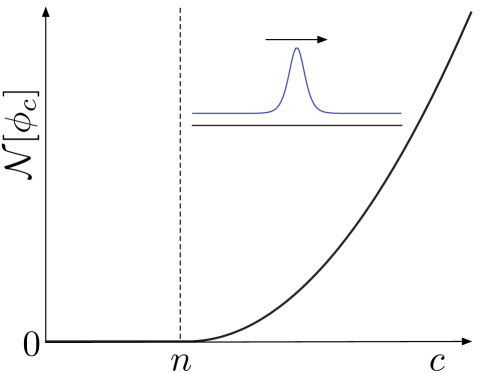
Figure 2: A diagram of $\mathcal{N}[\phi_{c}]$. $\mathcal{N}[\phi_{c}]$ and $d/dc\mathcal{N}[\phi_{c}]$ are zero at $c=n$. For $c\leq n$, there are not solitary waves.

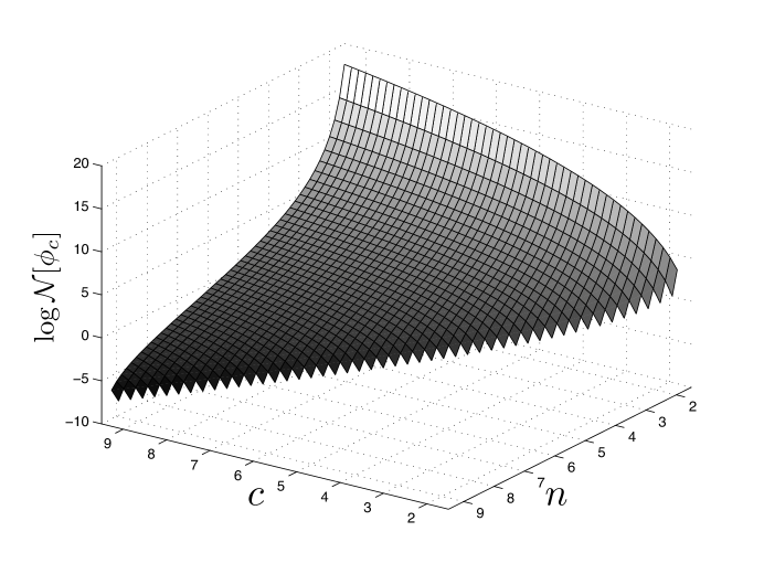
Figure 3: A plot of $\log\mathcal{N}[\phi_{c}]$, as a function of both $c$ and $n$, $c>n>1$, for the set $(c,n)\in[1.5,9.5]\times[1.5,9.5]$. It is monotonic in both arguments, and in particular, increasing in $c$ for fixed $n$.

4 Orbital Stability and Global Existence

4.1 Constraints of the Flow

Under appropriate restrictions on our function space, $L_{c}$ will be a positive definite operator, allowing us to conclude orbital stability. This is accomplished via two constraints discussed in the following two sections, 4.1.1 and 4.1.2.

4.1.1 The $\mathcal{N}$ Invariant

We would like to assume $\mathcal{N}[\phi]=\mathcal{N}[\phi_{c}]$, and use this as a constraint, as Benjamin did in [3]. This is of course not true for arbitrary ${H^{1}}$ perturbations. Following, [4], we show that for $\phi$ sufficiently close to $\phi_{c}$, we can find nearby solitary wave $\phi_{c^{\prime}}$ such that $\mathcal{N}[\phi]=\mathcal{N}[\phi_{c^{\prime}}]$.

Lemma 4.1

Given a solitary wave $\phi_{c}$, there exists $\delta_{c}>0$ such that for $\left\|u\right\|_{H^{1}}\leq\delta_{\mathcal{N}}$ there exists a $c^{\prime}$ such that $\mathcal{N}[u+\phi_{c}]=\mathcal{N}[\phi_{c^{\prime}}]$. Furthermore, there exists a constant, $K_{c}=K_{c}(\phi_{c})$ such that $\left|c-c^{\prime}\right|\leq K_{c}\left\|u\right\|_{H^{1}}$.

Proof: This is proved using the implicit function theorem. Let $\mathcal{F}$ be the functional $\mathcal{F}:{H^{1}}(\mathbb{R})\times\mathbb{R}\to\mathbb{R}$

$$\mathcal{F}[u,\Delta c]=\mathcal{N}[\phi_{c}+u]-\mathcal{N}[\phi_{c+\Delta c}]$$ (4.1)

$\mathcal{F}[\mathbf{0},0]=0$ and the Fréchet derivatives are

$$D\mathcal{F}[\mathbb{0},0]=\left(\left\langle c^{-1}(\phi_{c}^{n}-1),\cdot\right\rangle,\quad-\frac{d}{dc}\mathcal{N}[\phi_{c}]\right)$$ (4.2)

Both are bounded operators, and by Proposition 1 ,$\partial_{c}\mathcal{N}[\phi_{c}]\neq 0$. We may therefore apply the implicit function theorem for Banach spaces (see [14] for example), to conclude existence of an $\delta_{\mathcal{N}}>0$ and a $C^{1}$ mapping $\mathcal{G}:{H^{1}}\to\mathbb{R}$, such that if $\left\|u\right\|_{H^{1}}<\delta_{\mathcal{N}}$, then $\mathcal{F}[u,\mathcal{G}[u]]=0$. We then set $c^{\prime}=c+\mathcal{G}[u]$. Since this map is $C^{1}$, $\left|c-c^{\prime}\right|\leq K_{c}\left\|u\right\|_{H^{1}}$.

$\blacksquare$

If $\phi_{0}$ is our perturbed $\phi_{c}$, and $\left\|\phi_{0}-\phi_{c}\right\|\leq\delta_{c}$, then we may apply Lemma 4.1, to find $\phi_{c^{\prime}}$ such that $\mathcal{N}[\phi_{0}]=\mathcal{N}[\phi_{c^{\prime}}]$. Since $\mathrm{d}$ is a pseudo-metric on ${H^{1}}(\mathbb{R})$,

$$\mathrm{d}(\phi(t),\phi_{c})\leq\mathrm{d}(\phi(t),\phi_{c^{\prime}})+\mathrm{d}(\phi_{c},\phi_{c^{\prime}})$$

$\mathrm{d}(\phi_{c},\phi_{c^{\prime}})$ is time independent and

$$\mathrm{d}(\phi_{c},\phi_{c^{\prime}})\leq\left\|\phi_{c}-\phi_{c^{\prime}}\right\|_{H^{1}}\leq C\left|c-c^{\prime}\right|\leq C\left\|\phi_{0}-\phi_{c}\right\|_{H^{1}}$$

which may be made arbitrarily small. So it suffices to study the stability of $\phi_{c^{\prime}}$.

Examining how $\mathcal{N}[\phi]=\mathcal{N}[\phi_{c}]$ constrains the flow, first decompose $\phi$ as

$$\phi(x+x_{0},t)=\phi_{c}(x)+u(x,t)$$ (4.3)

the solitary wave and a perturbation, for some $x_{0}=x_{0}(t)$. Expanding $\mathcal{N}[\phi]=\mathcal{N}[\phi_{c}]$ about $\phi_{c}$,

$$\int_{-\infty}^{\infty}\left[I-\phi_{c}^{n}\partial_{x}\left(\phi_{c}^{n}\partial_{x}\cdot\right)\right]\left(\phi_{c}-1\right)udx=\left\langle\left[I-\phi_{c}^{n}\partial_{x}\left(\phi_{c}^{n}\partial_{x}\cdot\right)\right]\left(\phi_{c}-1\right),u\right\rangle=O(\left\|u\right\|_{H^{1}}^{2})$$

which we make formal in

Lemma 4.2

Given a solitary wave $\phi_{c}$, there exists a constant $C$ such that for any $\left\|u\right\|_{H^{1}}\leq\frac{1}{2}$,

$$\mathcal{N}[\phi_{c}+u]=\mathcal{N}[\phi_{c}]$$

$$\left|\left\langle\left[I-\phi_{c}^{n}\partial_{x}\left(\phi_{c}^{n}\partial_{x}\cdot\right)\right]\left(\phi_{c}-1\right),u\right\rangle\right|\leq C\left\|u\right\|_{H^{1}}^{2}$$ (4.4)

Remark 1

Since the right-hand side of (4.4) is quadratic in $\left\|u\right\|_{H^{1}}$, we view it as a near-orthogonality constraint.

4.1.2 The Sliding Metric and the Choice of $x_{0}(t)$

As discussed in [4] with regard to the sliding metric, (2.3), it is not true in general that the value of $y$ by which one function is translated to minimize the norm is be finite. We will show, under some additional appropriate assumptions that this is the case, see [4, 5].

Lemma 4.3

Given a solitary wave $\phi_{c}$, assume that a solution to $\eqref{eq:magma}$ $\phi$, $\phi-1\in C^{1}([0,T):H^{1}(\mathbb{R}))$, satisfies

$$\mathrm{d}(\phi(t),\phi_{c})<\left\|\phi_{c}-1\right\|_{H^{1}}$$ (4.5)

for $t<T$. Then the infimum of the function $\rho$,

$$\rho(y)=\left\|\phi(\cdot)-\phi_{c}(\cdot+y)\right\|_{H^{1}}^{2}$$ (4.6)

is achieved at a finite value of of $y\in\mathbb{R}$.

Proof: $\rho(y)$ is obviously continuous, and because $\phi(\cdot+y)-1\rightharpoonup 0$ in $H^{1}$ as $y\to\pm\infty$,

$$\lim_{y\to\pm\infty}\rho(y)=\left\|\phi-1\right\|_{H^{1}}^{2}+\left\|\phi_{c}-1\right\|_{H^{1}}^{2}>\left\|\phi_{c}-1\right\|_{H^{1}}^{2}$$

But by assumption,

$$\inf_{y\in\mathbb{R}}\rho(y)=\inf_{y\in\mathbb{R}}\left\|\phi(\cdot)-\phi_{c}(\cdot+y)\right\|_{H^{1}}^{2}=d(\phi,\phi_{c})^{2}<\left\|\phi_{c}-1\right\|_{H^{1}}^{2}$$

So there must be some finite $y_{0}$ such that $\rho(y_{0})<\rho(\pm\infty)$. By the continuity of $\rho$, there then exists an $x_{0}(t)$ at each $t<T$ such that $\rho(-x_{0}(t))\leq\rho(y)$ for all $y\in\mathbb{R}$.

$\blacksquare$

Remark 2

There therefore exists a function $x_{0}(t)$ such that

$$\mathrm{d}(\phi,\phi_{c})=\left\|\phi(\cdot,t)-\phi_{c}(\cdot-x_{0}(t))\right\|_{H^{1}}$$ (4.7)

Since $\phi_{c}$ is in fact smooth, so is $\rho(y)$, and hence $\rho^{\prime}(-x_{0}(t))=0$,

$$\int_{-\infty}^{\infty}\left[I-\partial_{x}^{2}\right]\partial_{x}\phi_{c}udx=\left\langle\left[I-\partial_{x}^{2}\right]\partial_{x}\phi_{c},u\right\rangle=0$$ (4.8)

where we used the decomposition (4.3). (4.8) is a second constraint on the perturbation to $\phi_{c}$, which together with the near-orthogonality condition (4.4), will be shown to yield local convexity of $\mathcal{E}$ near $\phi_{c}$.

4.2 Properties of the Linear Operator, $L_{c}$

Here we summarize properties of $L_{c}$, and exhibit the non-positivity of $L_{c}$.

Proposition 2

(Properties of the Linear Operator $L_{c}$) The linear second order operator defined by (3.5) has the following features:

(i)

$L_{c}$ is self adjoint, i.e.

$$L_{c}=L_{c}^{\dagger}$$ (4.9)

(ii)

$\partial_{x}\phi_{c}$ is an eigenvector of $L_{c}$ with eigenvalue zero

$$L_{c}\partial_{x}\phi_{c}=0$$ (4.10)

(iii)

$$L_{c}\partial_{c}\phi_{c}=-\left[I-\phi_{c}^{n}\partial_{x}\left(\phi_{c}^{n}\partial_{x}\cdot\right)\right]\left(\phi_{c}-1\right)=-c^{-1}\left(\phi_{c}^{n}-1\right)$$ (4.11)

(iv)

$$\left\langle L_{c}\partial_{c}\phi_{c},\partial_{c}\phi_{c}\right\rangle=-\frac{d}{dc}\mathcal{N}[\phi_{c}]$$ (4.12)

(v)

There exists $\lambda_{0}<0$ and $\psi_{0}\in L^{2}(\mathbb{R})$ such that

$$L_{c}\psi_{0}=\lambda_{0}\phi_{c}^{2n}\psi_{0}$$ (4.13)

i.e. $\psi_{0}$ is the ground state of $L_{c}$ with eigenvalue $\lambda_{0}$ of the generalized eigenvalue problem (4.13).

Proof: (i-iv) are trivial algebra and integration by parts. For (v), note that although $L_{c}$ is not in Sturm-Liouville form, if, given $h$, we let $\overline{h}=\phi_{c}^{n}h$,

$$\phi^{-n}L_{c}h=-c\partial_{x}^{2}\tilde{h}+\phi_{c}^{-2n}\left[c-n\phi^{n-1}-nc\phi_{c}^{n-1}\partial_{x}\left(\phi_{c}^{n}\partial_{x}\phi_{c}\right)\right]\tilde{h}=\overline{L}_{c}\overline{h}$$

$\overline{L}_{c}$ is in standard Sturm-Liouville form, and it has a zero eigenvector, $\phi_{c}^{n}\partial_{x}\phi_{c}$. Since this has one zero crossing, by oscillation theory (see [6], amongst others), we know there exists a ground state for $\overline{L}_{c}$, which we will denote by $\overline{\psi_{0}}$ with a negative eigenvalue, $\lambda_{0}$. In turn, $L_{c}$ has a generalized eigenvector $\psi_{0}=\phi_{c}^{-n}\overline{\psi_{0}}$ with eigenvalue $\lambda_{0}$, so

$$L_{c}\psi_{0}=\lambda_{0}\phi_{c}^{2n}\psi_{0}$$

We know this is the ground state of $L_{c}$ because if there existed some other $\psi$ with eigenvalue $\lambda<\lambda_{0}$, $\overline{\psi}=\phi^{n}\psi$ would be an eigenvector of $\overline{L}_{c}$ with eigenvalue $\lambda$, which contradicts $\overline{\psi_{0}}$ being the ground state of $\overline{L}_{c}$.

$\blacksquare$

We will now prove that with the constraints introduced in the previous section, (3.5) admits the estimate

$$\left|\Delta\mathcal{E}\right|\geq\frac{1}{2}\left\langle L_{c}u,u\right\rangle\geq C\left\|u\right\|_{H^{1}}^{2}+O\left(\left\|u\right\|_{H^{1}}^{3}\right)$$

Defining the two vectors in $L^{2}$,

$$\xi_{1} = \left[I-\phi_{c}^{n}\partial_{x}\left(\phi_{c}^{n}\partial_{x}\cdot\right)\right]\left(\phi_{c}-1\right)$$ (4.14)

$$\xi_{2} = \left[I-\partial_{x}^{2}\right]\partial_{x}\phi_{c}$$ (4.15)

Proposition 3

Let

$$\mathcal{A}=\left\{f\in{H^{1}}:\quad\left\|\phi_{c}^{n}f\right\|_{L^{2}}=1\quad\mbox{and}\quad f\bot\xi_{1}\right\}$$

Then

$$\inf_{f\in\mathcal{A}}\left\langle L_{c}f,f\right\rangle=0$$

Proof: Following,[24, 25] , let $\alpha=\inf\left\langle L_{c}f,f\right\rangle$, taken over $\mathcal{A}$. Assume $\alpha<0$, and let us treat this as a constrained minimization problem. From the theory of Lagrange multipliers, there exist $f_{\star}$, $\beta_{\star}$ such that

$$\left(L_{c}-\alpha\phi^{2n}\right)f_{\star}=\beta_{\star}\xi_{1}$$ (4.16)

If $\beta_{\star}$ is zero, then $\alpha=\lambda_{0}$ which implies $f_{\star}$ is some multiple of the ground state $\psi_{0}$, as defined in Proposition 2. But since $\psi_{0}$ and $\xi_{1}$ are both even functions,

$$\left\langle f_{\star},\xi_{1}\right\rangle\propto\left\langle\psi_{0},\xi_{1}\right\rangle\neq 0$$

and this contradicts the assumption that $f_{\star}$ is orthogonal to $\xi_{1}$. Therefore, $\beta_{\star}\neq 0$. If $\alpha=\lambda_{0}$, then, taking the inner product of both sides of (4.16) with the ground state,

$$0=\left\langle f_{\star},\left(L_{c}-\lambda_{0}\phi^{2n}\right)\psi_{0}\right\rangle=\left\langle\left(L_{c}-\alpha\phi^{2n}\right)f_{\star},\psi_{0}\right\rangle=\beta_{\star}\left\langle\xi_{1},\psi_{0}\right\rangle=\beta_{\star}\left\langle\frac{1}{c}\left(\phi_{c}^{n}-1\right),\psi_{0}\right\rangle\neq 0$$

So $\lambda_{0}<\alpha<0$.

Let $g(\lambda)$ be defined as

$$g(\lambda)=\left\langle\left(L_{c}-\lambda\phi^{2n}\right)^{-1}\xi_{1},\xi_{1}\right\rangle$$

on the interval $(\lambda_{0},0]$. Note

$$g^{\prime}(\lambda) = \left\langle\phi_{c}^{2n}\left(L_{c}-\lambda\phi^{2n}\right)^{-1}\xi_{1},\left(L_{c}-\lambda\phi^{2n}\right)^{-1}\xi_{1}\right\rangle$$

$$= \left\|\phi_{c}^{n}\left(L_{c}-\lambda\phi^{2n}\right)^{-1}\xi_{1}\right\|_{L^{2}(\mathbb{R})}^{2}>0$$

so $g$ is increasing on this interval. Additionally,

$$g(0)=-\frac{d}{dc}\mathcal{N}[\phi_{c}]<0$$

by Proposition 1. This implies that $g(\alpha)<0$. But

$$g(\alpha)=\frac{1}{\beta_{\star}}\left\langle f_{\star},\xi_{1}\right\rangle=0$$

Therefore $\alpha=0$.

$\blacksquare$

Remark 3

It is here that we see the importance of the slope condition on $\mathcal{N}$ with respect to $c$. Also, we see from Figure 3 (a) and (b), and the exact computation when $n=2$, that as $c\to n$, $\partial_{c}\mathcal{N}[\phi_{c}]\to 0$. There is a bifurcation point at $c=n$, for there are not solitary waves for $c\leq n$, but under linearization about $\phi\equiv 1$,there are plane waves with group velocity $\leq n$; this is cartooned in Figure 3 (a). The sign of the derivative of this functional with respect to $c$ was previously used in [1] to conclude linear instability of one dimensional solitary waves in two spatial dimensions of (1.1), when $n=3$ and $m=0$.

Proposition 4

Let

$$\mathcal{B}=\left\{f\in\mathcal{A}:\quad f\bot\xi_{2}\right\}=\left\{f\in{H^{1}}:\quad\left\|\phi_{c}^{n}f\right\|_{L_{2}}=1,\quad f\bot\xi_{1},\quad f\bot\xi_{2}\right\}$$

Then

$$\inf_{f\in\mathcal{B}}\left\langle L_{c}f,f\right\rangle>0$$

Proof: Let

$$\alpha=\inf_{f\in\mathcal{B}}\left\langle L_{c}f,f\right\rangle$$

Since $\mathcal{B}\subset\mathcal{A}$, $\alpha\geq 0$ by the previous Proposition. Assume that $\alpha=0$ and this minimum is achieved at $f_{\star}$. Again, by the theory of Lagrange multipliers,

$$L_{c}f_{\star}=\beta_{\star}\xi_{1}+\gamma_{\star}\xi_{2}$$

Taking the inner product of both $L_{c}f_{\star}$ with $\partial_{x}\phi_{c}$,

$$0=\left\langle f_{\star},L_{c}\partial_{x}f_{c}\right\rangle=\left\langle L_{c}f_{\star},\partial_{x}f_{c}\right\rangle=\beta_{\star}\left\langle\xi_{1},\partial_{x}\phi_{c}\right\rangle+\gamma_{\star}\left\langle\xi_{2},\partial_{x}\phi_{c}\right\rangle$$

Since $\xi_{1}$ is an even function and $\partial_{x}\phi_{c}$ is odd, $\left\langle\xi_{1},\partial_{x}\phi_{c}\right\rangle=0$, hence $\gamma_{\star}=0$, implying

$$f_{\star}=\kappa_{\star}\partial_{x}\phi_{c}-\beta_{\star}\partial_{c}\phi_{c}$$

Taking the inner product of $f_{\star}$ with $\xi_{1}$,

$$0=\left\langle f_{\star},\xi_{1}\right\rangle=-\beta_{\star}\frac{d}{dc}\mathcal{N}[\phi_{c}]\neq 0$$

Therefore $\alpha>0$.

$\blacksquare$

Corollary 2

There exists a constant $C>0$ such that for all $f\in H^{1}(\mathbb{R})$ orthogonal to both $\xi_{1}$ and $\xi_{2}$

$$\left\langle L_{c}f,f\right\rangle\geq C\left\|f\right\|_{L^{2}}^{2}$$

which further implies

$$\left\langle L_{c}f,f\right\rangle\geq C^{\prime}\left\|f\right\|_{H^{1}}^{2}$$

Proof: The first part is obvious by Proposition 4. To prove the second inequality, let us express $L_{c}$ using (3.5) as

$$L_{c}=-c\partial_{x}\left(\phi_{c}^{2n}\partial_{x}\cdot\right)+V(x)$$

Then

$$\left\langle L_{c}f,f\right\rangle = c\left\langle\phi_{c}^{n}\partial_{x}f,\phi_{c}^{n}\partial_{x}f\right\rangle+\left\langle Vf,f\right\rangle$$

$$\geq \left\|\partial_{x}f\right\|_{L^{2}}^{2}-\left\|V\right\|_{L^{\infty}}\left\|f\right\|_{L^{2}}^{2}$$

$$\geq \left\|\partial_{x}f\right\|_{L^{2}}^{2}-C^{-1}\left\|V\right\|_{L^{\infty}}\left\langle L_{c}f,f\right\rangle$$

hence

$$\left\langle L_{c}f,f\right\rangle\geq\left(1+C^{-1}\left\|V\right\|_{L^{\infty}}\right)^{-1}\left\|\partial_{x}f\right\|_{L^{2}}^{2}$$

and the inequality follows.

$\blacksquare$

Proposition 5

Given a solitary wave $\phi_{c}$ with $c>n>1$ for (1.1), there exist positive constants $C_{2}$, $C_{3}$ such that for all $u\in{H^{1}}$ satisfying

$$\left\|u\right\|_{H^{1}} \leq \frac{1}{2}$$ (4.17)

$$\mathcal{N}[\phi_{c}+u] = \mathcal{N}[\phi_{c}]$$ (4.18)

$$\left\langle\xi_{2},u\right\rangle = 0$$ (4.19)

$\xi_{2}$ given by (4.15), we have

$$\left\langle L_{c}u,u\right\rangle\geq C_{2}\left\|u\right\|_{H^{1}}^{2}-C_{3}\left\|u\right\|_{H^{1}}^{3}$$ (4.20)

Proof: Let $u=u_{\bot}+u_{\|}$ where

$$u_{\|}=\left\langle u,\xi_{1}\right\rangle\xi_{1}$$

and

$$u_{\bot}=u-u_{\|}=u-\left\langle u,\xi_{1}\right\rangle\xi_{1}$$

Then

$$\left\langle L_{c}u,u\right\rangle=\left\langle L_{c}\left(u_{\bot}+u_{\|}\right),u_{\bot}+u_{\|}\right\rangle=\left\langle L_{c}u_{\bot},u_{\bot}\right\rangle+2\left\langle L_{c}u_{\bot},u_{\|}\right\rangle+\left\langle u_{\|},u_{\|}\right\rangle$$

By Corollary 2 and Lemma 4.4,

$$\left\langle L_{c}u_{\bot},u_{\bot}\right\rangle \geq C\left\|u_{\bot}\right\|_{H^{1}}^{2}=C\left[\left\|u\right\|_{H^{1}}^{2}-2\left\langle u,u_{\|}\right\rangle-2\left\langle\partial_{x}u,\partial_{x}u_{\|}\right\rangle+\left\|u_{\|}\right\|_{H^{1}}^{2}\right]$$ (4.21)

$$= C\left[\left\|u\right\|_{H^{1}}^{2}-2\left\langle u,\xi_{1}\right\rangle^{2}-2\left\langle\partial_{x}u,\xi_{1}\right\rangle\left\langle u,\xi_{1}\right\rangle+\left\langle u,\xi_{1}\right\rangle^{2}\left\|\xi_{1}\right\|_{H^{1}}^{2}\right]$$

$$\geq C\left\|u\right\|_{{H^{1}}}^{2}-D\left\|u\right\|_{H^{1}}^{3}$$

The other two terms follow more easily

$$\left\langle L_{c}u_{\|},u_{\|}\right\rangle = \left\langle u,\xi_{1}\right\rangle^{2}\left\langle L_{c}\xi_{1},\xi_{1}\right\rangle$$ (4.22)

$$\geq -D\left\|u\right\|_{H^{1}}^{4}$$

$$\left\langle L_{c}u_{\bot},u_{\|}\right\rangle = \left\langle L_{c}u,u_{\|}\right\rangle-\left\langle L_{c}u_{\|},u_{\|}\right\rangle=\left\langle u,\xi_{1}\right\rangle\left\langle u,L_{c}\xi_{1}\right\rangle+\left\langle u,\xi_{2}\right\rangle\left\langle u,L_{c}\xi_{2}\right\rangle$$ (4.23)

$$\geq -D\left\|u\right\|_{H^{1}}^{3}$$

(4.20) then follows immediately from (4.21),(4.22), and (4.23).

$\blacksquare$

Remark 4

Using the estimate (4.20) together with (3.6),

$$\left|\Delta\mathcal{E}\right| \geq \mathcal{E}[\phi_{c}+u]-\mathcal{E}[\phi_{c}]\geq\frac{1}{2}\left\langle L_{c}u,u\right\rangle-D_{3}\left\|u\right\|_{H^{1}}^{3}$$ (4.24)

$$\geq \frac{1}{2}C_{2}\left\|u\right\|_{H^{1}}^{2}-\left(\frac{1}{2}C_{2}+D_{3}\right)\left\|u\right\|_{H^{1}}^{3}\equiv p_{-}\left(\left\|u\right\|_{H^{1}}\right)$$

The polynomial $p_{-}$ will be important in the next section.

4.3 Proof of Orbital Stability and Global Existence in Time

Unlike non-degenerate equations, such as KdV and BBM, we need to control $\left\|1/\phi\right\|_{L^{\infty}}$ in our existence proof, hence the additional condition appearing in Theorem 2.1. It is a lack of a priori bounds on this quantity that currently prevents a global existence proof for general $(n,m)$; this matter is discussed in [20]. However, we are able to prove, in tandem with nonlinear stability, global existence in time for data in a neighborhood of a solitary wave.

4.3.1 Proof of Main Theorem

Let a particular solitary wave $\phi_{c}$ be given for some $c>n>1$, and let $\phi$ be a solution to (1.1). First we will consider the case where $\mathcal{N}[\phi]=\mathcal{N}[\phi_{c}]$; this will then be relaxed.

For $u$ satisfying (4.17), (4.18), and (4.19), the perturbation will satisfy the two inequalities

$$p_{-}\left(\left\|u\right\|_{H^{1}}\right)\leq\left|\Delta\mathcal{E}\right|\leq p_{+}\left(\left\|u\right\|_{H^{1}}\right)$$

$p_{\pm}$ defined in (3.7) and (4.24). Since $\Delta\mathcal{E}$ is time independent, if the perturbation at time $t=0$ is sufficiently small, $\left|\Delta\mathcal{E}\right|$ may be made arbitrarily small. Provided conditions (4.17), (4.18), and (4.19) continue to hold, this will constrain $\left\|u\right\|_{H^{1}}$ through $p_{-}$.

Let $\varepsilon_{\star}$ be defined as

$$\varepsilon_{\star}=\min\left\{\frac{1}{4},\frac{1}{2}\left\|\phi_{c}-1\right\|_{H^{1}},\frac{C_{2}}{3\left(C_{3}+2D_{3}\right)}\right\}$$ (4.25)

which depends only on $\phi_{c}$. The significance of the three quantities is:

• $1/4$ will ensure $\phi$ is bounded away from zero, as needed by our existence theory.

• $1/2\left\|\phi_{c}-1\right\|_{H^{1}}$ will ensure the value at which the sliding metric is minimized is finite; see Lemma 4.3.

• $C_{2}/(3C_{3}+6D_{3})$ will ensure that the perturbation reamins to the left of the peak of the polynomial $p_{-}$.

Let $\varepsilon\leq\varepsilon_{\star}$ and let $\delta>0$ be sufficiently small such that

$$\delta<\varepsilon$$ (4.26)

$$p_{+}(\delta)<p_{-}(\varepsilon)$$ (4.27)

Letting $\phi(t=0)\equiv\phi_{0}$, assume there is $x_{0}\in\mathbb{R}$ such that

$$\left\|\phi_{0}-\phi_{c}(\cdot+x_{0})\right\|_{H^{1}}=\left\|u_{0}\right\|_{H^{1}}<\delta$$

$\phi-1\in C^{1}\left([0,T_{\max});{H^{1}}\right)$. With these choices of $\delta$, $\varepsilon$, and $\varepsilon_{\star}$, we will show that for $t\in[0,T_{\max})$, $\mathrm{d}(\phi(t),\phi_{c})<\varepsilon$.

Let

$$\mathcal{I}=\left\{t:\mathrm{d}(\phi(t^{\prime}),\phi_{c})<{\quad}_{\varepsilon}\mbox{for $t^{\prime}<t$.}\right\}$$

We will use $\mathcal{I}$ to prove the theorem by contradiction as follows:

• Use continuous dependence upon the data of solutions of (1.1) to prove that $\mathcal{I}$ is not empty.

• Seek the maximal time $T_{0}$ in $\mathcal{I}$. If it is not $T_{\max}$, we will show that there is some time interval beyond $T_{0}$ for which $\mathrm{d}(\phi(t),\phi_{c})<2\varepsilon$.

• Prove that for any $t$ such that $\mathrm{d}(\phi(t),\phi_{c})<2\varepsilon$, in fact $\mathrm{d}(\phi(t),\phi_{c})<\varepsilon$, producing the contradiction.

First we prove that $\mathcal{I}$ is not empty. This is an application of Theorem 2.1.

$$\left\|\phi_{0}-1\right\|_{H^{1}}\leq\frac{3}{2}\left\|\phi_{c}-1\right\|_{H^{1}}\quad\mbox{and}\quad\left\|\frac{1}{\phi_{0}}\right\|_{L^{\infty}}\leq\frac{4}{3}$$

Taking $R=3/2\left\|\phi_{c}-1\right\|_{H^{1}}$, $\alpha=3/8$, we know from part (a) of Theorem 2.1, that $\left\|\phi(t)-1\right\|\leq 2R$ and $\left\|1/\phi(t)\right\|_{L^{\infty}}\leq 1/\alpha$ up till at least $T_{\mathrm{exist.}}(R,\alpha)>0$ and $T_{\max}\geq T_{\mathrm{exist.}}$.

By part (c) of the same Theorem, we have a constant $K_{\mathrm{cont.}}=K_{\mathrm{cont.}}(R,\alpha)$, such that

$$\left\|\phi(\cdot,t)-\phi_{c}(\cdot-ct+x_{0})\right\|_{H^{1}}\leq\left\|\phi_{0}-\phi_{c}(\cdot+x_{0})\right\|_{H^{1}}e^{K_{\mathrm{cont.}}t}<\delta e^{K_{\mathrm{cont.}}t}$$

Taking $t$ sufficiently small, there is some time interval over which $\phi$ is within $\varepsilon$ of $\phi_{c}$.

Let

$$T_{0}=\sup\mathcal{I}$$ (4.28)

Suppose $T_{0}<T_{\max}$. For any $t<T_{0}$,

$$\mathrm{d}(\phi(t),\phi_{c})<{\leq}_{\varepsilon}\frac{1}{2}\left\|\phi_{c}-1\right\|_{H^{1}}$$

Lemma 4.3 asserts there exists $x_{0}(t)\in\mathbb{R}$ such that

$$\mathrm{d}(\phi(t),\phi_{c})=\left\|\phi(\cdot,t)-\phi_{c}(\cdot+x_{0}(t))\right\|_{H^{1}}<\varepsilon$$

Furthermore, for all $t<T_{0}$, we have again

$$\left\|\phi(t)-1\right\|_{H^{1}}\leq\frac{3}{2}\left\|\phi_{c}-1\right\|_{H^{1}}\quad\mbox{and}\quad\left\|\frac{1}{\phi(t)}\right\|_{H^{1}}\leq\frac{4}{3}$$

We use these bounds to control how far $\phi$ can deviate from $\phi_{c}$ beyond $T_{0}$. Taking $R=3/2\left\|\phi_{c}-1\right\|_{H^{1}}$ and $\alpha=3/8$, there exists $T_{\mathrm{exist.}}(R,\alpha)>0$ such that $\phi(t)$, for $t<T_{0}$, may be continued in time by the amount $T_{\mathrm{exist.}}$ and will satisfy $\left\|\phi(t)-1\right\|\leq 2R$, and $\left\|1/\phi(t)\right\|_{L^{\infty}}\leq 1/\alpha$. Because the solution is unique, these bounds apply to $\phi$ for $t<T_{0}+T_{\mathrm{exist.}}$.

With this control on norms, we let $t_{1}<T_{0}$ be a new starting point, and apply part (c) of Theorem 2.1

$$\left\|\phi(\cdot,t)-\phi_{c}(\cdot-ct+x_{0}(t_{1}))\right\|_{H^{1}}\leq\left\|\phi(\cdot,t_{1})-\phi_{c}(\cdot+x_{0}(t_{1})\right\|_{H^{1}}e^{K_{\mathrm{cont.}}(t-t_{1})}<{e}_{\varepsilon}^{K_{\mathrm{cont.}}(t-t_{1})}$$

Making $t_{1}$ sufficiently close to $T_{0}$, we can find $T_{2}>T_{0}$ for which

$$\left\|\phi(\cdot,t)-\phi_{c}(\cdot-ct+x_{0}(t_{1}))\right\|_{H^{1}}=\left\|u(t)\right\|_{H^{1}}<2\varepsilon$$

for $t<T_{2}$. We claim this implies the stricter estimate $\left\|\phi(\cdot,t)-\phi_{c}(\cdot-ct+x_{0}(t_{1}))\right\|_{H^{1}}<\varepsilon$ for $T_{0}<t<T_{2}$.

$2\varepsilon\leq 2\varepsilon_{\star}\leq\left\|\phi_{c}-1\right\|_{H^{1}}$; applying Lemma 4.3 to find $x_{0}(t)$ again, and then decompose our solution via (4.3). As noted in the remark following Lemma 4.3, this perturbation satisfies $\left\langle\xi_{2},u\right\rangle=0$. $\mathcal{N}[\phi]=\mathcal{N}[\phi_{c}]$ and

$$\left\|u\right\|_{H^{1}}<2\varepsilon\leq 2\varepsilon_{\star}\frac{1}{2}$$

Therefore $u$ satisfies the neccessary conditions to apply Proposition 4.20,

$$p_{-}\left(\left\|u\right\|_{H^{1}}\right)\leq\left|\Delta\mathcal{E}\right|\leq p_{+}(\delta)<p_{-}(\varepsilon)$$

Because $\left\|u\right\|_{H^{1}}<2{\leq}_{\varepsilon}2\varepsilon_{\star}\leq 2C_{2}/(3C_{3}+6D_{3})$, it sits remains to the left of the peak of $p_{-}$;

$$\left\|u(t)\right\|_{H^{1}}=\mathrm{d}(\phi(t),\phi_{c})<\varepsilon$$

This holds for $T_{0}<t<T_{2}$, $T_{0}<T$ so we have a contradiction and conclude $\mathrm{d}(\phi(t),\phi_{c})<\varepsilon$ for all $t<T$.

Now we relax $\mathcal{N}[\phi_{0}]=\mathcal{N}[\phi_{c}]$. First apply Lemma 4.1 to $\phi_{c}$, to find $\delta_{c}$ that will define the ${H^{1}}$ neighborhood about the origin where the initial perturbation must reside. Let $K$ be the constant such that

$$\left\|\phi_{c}-\phi_{c^{\prime}}\right\|_{H^{1}}\leq\tilde{K}\left|c-c^{\prime}\right|\leq\tilde{K}K_{c}\left\|u\right\|_{H^{1}}=K\left\|u\right\|_{H^{1}},$$

where $K_{c}$ is from Lemma 4.1. We will seek a new wave $\phi_{c^{\prime}}$ with which to apply the preceding argument; however, $\varepsilon_{\star}$ and the polynomials $p_{\pm}$ will be determined by $\phi_{c^{\prime}}$. But $\phi_{c^{\prime}}$ is determined by $\phi_{0}$ and we have not yet found all the bounds $\phi_{0}$ must satisfy. Uniform control is needed. Using $\mathcal{G}$, the implicit function associated with Lemma 4.1, let

$$c_{\min} = \min_{\left\|u\right\|_{H^{1}}<\delta_{c}}\mathcal{G}[u]$$

$$c_{\max} = \max_{\left\|u\right\|_{H^{1}}<\delta_{c}}\mathcal{G}[u]$$

and let

$$\varepsilon_{\star}^{\prime}=\min_{c\in[c_{\min},c_{\max}]}\varepsilon_{\star}(\phi_{c})$$

Similarly, the coefficients of $p_{\pm}$ may be chosen such that

$$p^{\prime}_{-}\left(\left\|u\right\|_{H^{1}}\right)\leq\left|\mathcal{E}[\phi_{c}+u]-\mathcal{E}[\phi_{c}]\right|=\left|\Delta\mathcal{E}\right|\leq p^{\prime}_{+}\left(\left\|u\right\|_{H^{1}}\right)$$

for all $c\in[c_{\min},c_{\max}]$, $\left\|u\right\|_{H^{1}}<\min\{\delta_{c},\frac{1}{2}\}$ (the $\frac{1}{2}$ is required by Lemma 3.1).

Given $\phi_{c}$, let $\varepsilon_{\star}^{\prime}$ be as above. Let $\varepsilon_{\star}=\varepsilon_{\star}^{\prime}(1+K)$. Take $\varepsilon\leq\varepsilon_{\star}$, and then set $\varepsilon^{\prime}=\varepsilon/(1+K)$. Choose $\delta$ such that

$$\delta < \delta_{c}$$ (4.29)

$$(1+K)\delta < \varepsilon^{\prime}$$ (4.30)

$$p^{\prime}_{+}((1+K)\delta) < p^{\prime}_{-}(\varepsilon^{\prime})$$ (4.31)

and let $\delta^{\prime}=\delta(1+K)$.

Assume

$$\left\|\phi_{0}-\phi_{c}(\cdot+x_{0})\right\|_{H^{1}}<\delta$$

Let $\phi_{c^{\prime}}$ be the neighboring solitary wave for which $\mathcal{N}[\phi_{0}]=\mathcal{N}[\phi_{c^{\prime}}]$. Note $\phi_{0}$ is also close to $\phi_{c^{\prime}}$,

$$\left\|\phi_{0}(\cdot)-\phi_{c^{\prime}}(\cdot+x_{0})\right\|_{H^{1}}\leq\left\|\phi_{0}(\cdot)-\phi_{c}(\cdot+x_{0})\right\|_{H^{1}}+\left\|\phi_{c^{\prime}}-\phi_{c}\right\|_{H^{1}}<(1+K)\delta=\delta^{\prime}$$

Because $\delta^{\prime}<\varepsilon^{\prime}$ and $p^{\prime}_{+}(\delta^{\prime})<p^{\prime}_{-}(\varepsilon^{\prime})$, $\varepsilon^{\prime}\leq\varepsilon_{\star}^{\prime}$, we may apply the previous argument, to conclude

$$\mathrm{d}(\phi(t),\phi_{c^{\prime}})<\varepsilon^{\prime}$$

for $t\in[0,T_{\max})$. Finally,

$$\mathrm{d}(\phi(t),\phi_{c})\leq\mathrm{d}(\phi(t),\phi_{c^{\prime}})+\mathrm{d}(\phi_{c^{\prime}},\phi_{c})<{{}^{\prime}}_{\varepsilon}+K\delta\leq{{}^{\prime}}_{\varepsilon}+K\delta^{\prime}<(1+K)\varepsilon^{\prime}=\varepsilon$$

$\blacksquare$

4.3.2 Proof of Corollary 1

Now we will prove global existence in time for a data in a neighborhood of a solitary wave. Given a solitary wave $\phi_{c}$, $\varepsilon\leq\varepsilon_{\star}$, and any function $\phi$ such that

$$\left\|\phi_{0}(\cdot)-\phi_{c}(\cdot-x_{0})\right\|_{H^{1}}<\delta$$

Let $T_{\max}$ be the maximal time of existence of $\phi$, the solution emanating from $\phi_{0}$. Suppose $T_{\max}<\infty$.

By Theorem 2.4, for all $t<T_{\max}$,

$$\mathrm{d}(\phi(t),\phi_{c})<\varepsilon$$

which implies

$$\phi(t)>1-\varepsilon\geq 1/2$$

$$\left\|\phi(t)-1\right\|_{H^{1}}<\varepsilon+\left\|\phi_{c}-1\right\|_{H^{1}}<2\left\|\phi_{c}-1\right\|_{H^{1}}$$

and hence

$$\left\|\phi-1\right\|_{H^{1}}+\left\|\frac{1}{\phi}\right\|_{L^{\infty}}<\frac{1}{2\left\|\phi_{c}-1\right\|_{H^{1}}}+2$$

for all $t<T_{\max}$. But $\phi$ is $C^{1}$ in time, and since $T_{\max}<\infty$,

$$\lim_{t\to T_{\max}}\left\|\phi-1\right\|_{H^{1}}+\left\|\frac{1}{\phi}\right\|_{L^{\infty}}=\infty$$

a contradiction. Therefore $T_{\max}=\infty$, and furthermore, by Theorem 2.4 again,

$$\mathrm{d}(\phi(t),\phi_{c})<\varepsilon$$

for all time.

$\blacksquare$

5 Relation to Compacton Equations

Compactons, robust compactly supported solitary waves, were first identified in [16] in a generalization of KdV, $K(m,n)$,

$$\partial_{t}u+\partial_{x}\left(u^{m}\right)+\frac{1}{n}\partial_{x}^{3}\left(u^{n}\right)=0$$

$K(m,n)$ has been further generalized to $C_{1}(m,a+b)$,

$$\partial_{t}u+\partial_{x}\left(u^{m}\right)+\frac{1}{b}\partial_{x}\left[u^{a}\partial_{x}^{2}\left(u^{b}\right)\right]=0$$ (5.1)

discussed in [15], which are known admit traveling wave solutions of speed $c\geq 0$, compactly supported in space. In turn, this has been generalized to the multidimensional case, $C_{N}(m,a+b)$, in [15, 17].

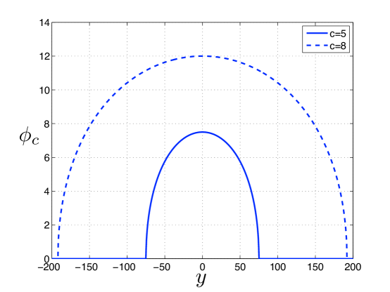
Figure 4: Compacton solutions to (1.1) with $n=2$, $m=-2$ for $c=5$ and $c=8$. Faster compactons are both broader and taller.

Like (1.1), (5.1) is a nonlinearly dispersive wave equation. Indeed, (1.1) may be written as

$$\partial_{t}\phi+\partial_{x}\left(\phi^{n}\right)-\frac{1}{1-m}\partial_{x}\left[\phi^{n}\partial_{x}\partial_{t}\left(\phi^{1-m}\right)\right]=0$$ (5.2)

which, upon setting $a=n$ and $b=1-m$, resembles (5.1) up to one $\partial_{x}$ becoming $-\partial_{t}$. It was the recognition of this similarity between these two equations that led the authors to discover that just as (5.1) is Hamiltonian for $b-a=1$, so too is (1.1) when $1-m-n=1$, $n+m=0$. (1.1) may be interpreted as a generalization of the BBM equation, just as (5.1) is a generalization of KdV. In addition, (1.1) also possesses compacton solutions, pictured in Figure 4.

Equation (5.1) has a second set of Hamiltonian cases when $b-a=\frac{1}{2}$, which is related to the property that the density of the generalized momentum of (5.1)

$$\int u^{1+b-a}$$

is a mapping of a (5.1) into another such equation. The generalized momentum of (1.1), (3.1), not being a monomial, lacks this property. Note also that (1.1) could be further generalized by letting the the nonlinearity in the $(\phi^{n})_{x}$ vary independently of the dispersive term; however, for physical reasons related to its derivation, we leave it as is.

We now construct compactons. Starting with (5.2), we integrate it up, assuming there exists $y_{\max}>0$, such that for $\left|y\right|>y_{\max}$, $Q_{c}=0$. Then

$$-cQ_{c}+Q_{c}^{n}+\frac{c}{1-m}Q_{c}^{n}\partial_{y}^{2}\left(Q_{c}^{1-m}\right)=0\quad\mbox{for $\left|y\right|\leq y_{\max}$}$$ (5.3)

with boundary conditions $Q_{c}=0$ at $\left|y\right|=y_{\max}$.

Introducing the scaling

$$Q_{c}(y)=c^{\frac{1}{n-1}}U(\sqrt{1-m}c^{-\frac{n-m}{2(n-1)}}y)^{\frac{1}{1-m}}=c^{\frac{1}{n-1}}U(\xi)^{\frac{1}{1-m}}$$ (5.4)

into (5.3), $U$ solves

$$-U^{-\frac{n-1}{1-m}}+1+\partial_{\xi}^{2}U=0$$ (5.5)

Remark 5

Assuming $n>1$, the scaling, (5.4), highlights three distinct regimes

• If $n>m$, faster waves are taller and narrower.

• If $n<m$, faster waves are taller and broader.

• If $n=m$, faster waves are taller, but all waves have the same width.

Integrating (5.5) again,

$$\frac{1}{2}\left(\partial_{\xi}U\right)^{2}+\mathrm{V}(U;\beta)=0$$

where the potential, $\mathrm{V}$,

$$\mathrm{V}(U;\beta)=\left\{\begin{array}[]{cc}U-\frac{1}{1-\beta}U^{1-\beta},&\mbox{ if }\beta\neq 1\\ U-\log U,&\mbox{ if }\beta=1\end{array}\right.$$

and $\beta=(n-1)/(1-m)$.

Representative cases for $\beta\geq 1$, $0<\beta<1$ and $\beta<0$ are illustrated Figure 5. Compactons are homoclinic orbits in the $(U,U^{\prime})$ phase plane connecting the equilibrium point $(0,0)$ to itself in finite time. This corresponds to $\mathrm{V}$ having a potential well between $U=0$ and some $U_{\max}>0$. Such a well exists only for $0<\beta<1$; see Figure 5.

In terms of $n$ and $m$, for $n>1$, $0<\beta<1$ corresponds to $n+m<2$, which obviously includes the Hamiltonian case of (1.2), (1.3), (1.4); $n+m=0$. With regard to Remark 5, because we have assumed $n>1$, we are in regime where faster waves are both taller and broader.

We note that several examples of compactly supported solutions of (1.1) were previously examined in [23, 22]. These included the exponents $(n,m)=(3,0),(4,0)$. The authors argued against the realization in nature of such solutions due to a stress singularity.

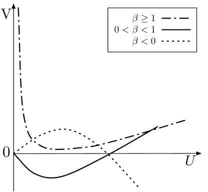
Figure 5: The different regimes of $\mathrm{P}$ for different $\beta$. We exclude $\beta=0$ because $\mathrm{P}(\beta=0)\equiv 0$.

Some solutions of (5.5), given implicitly by

$$-\frac{24U+10U^{4/5}+50U^{3/5}-125U^{2/5}}{6\sqrt{10U^{4/5}-8U}}=\left|\xi\right|\quad\mbox{for $\beta=\frac{1}{5}$}$$ (5.6)

$$\frac{-2U-3U^{2/3}+9\sqrt[3]{U}}{\sqrt{3U^{2/3}-2U}}=\left|\xi\right|\quad\mbox{for $\beta=\frac{1}{3}$}$$ (5.7)

$$-\frac{\sqrt[4]{U}\left(2\sqrt{\sqrt{U}-2}\log\left(\sqrt{\sqrt{U}-2}+\sqrt[4]{U}\right)+U^{3/4}-2\sqrt[4]{U}\right)}{\sqrt{\sqrt{U}-U/2}}=\left|\xi\right|\quad\mbox{for $\beta=\frac{1}{2}$}$$ (5.8)

and

$$U\in\left(0,\left(\frac{1}{1-\beta}\right)^{\frac{1}{\beta}}\right)$$

The compactons are a type of weak solution to (1.1), but the exact notion is still imprecise. Near the left edge of the compacton, $U\sim\left|\xi+\xi_{\max}\right|^{2/(1+\beta)}H(\xi+\xi_{\max})$, $H(x)$ the heavyside function. In the Hamiltonian case $Q_{c}\sim\left|y+y_{\max}\right|^{1/n}H(y+y_{\max})$. For $n\geq 2$, this will not have a square integrable derivative. They do satisfy the following definition, previously given in [20] for solutions of (1.1) that go to zero.

Definition 5.1

$\phi(x,t)$ is a solution of (1.1) if

$$\int_{0}^{\infty}\int_{-\infty}^{\infty} \Big{[} -\partial_{t}\psi(x,t)\phi(x,t)-\partial_{x}\psi(x,t)\phi(x,t)^{n}$$ (5.9)

$$+\frac{1}{1-m}\partial_{x}\psi(x,t)\phi(x,t)^{n}\partial_{x}\partial_{t}\left(\phi(x,t)^{1-m}\right)\Big{]}dxdt=0$$

for all $\psi(x,t)\in C^{\infty}_{0}(\mathbb{R}\times\mathbb{R}^{+})$, and such that both

$$\phi(x,t)\quad\mbox{and}\quad\phi(x,t)^{n}\partial_{x}\partial_{t}\left(\phi(x,t)^{1-m}\right)$$

are in $L^{1}_{loc}(\mathbb{R})$ in the $x$ coordinate.

Proposition 6

$Q_{c}$ is a solution of (1.1) in the sense of Definition 5.1.

Proof: For $\left|x-ct\right|>y_{\max}$, $Q_{c}\equiv 0$, and satisfies (5.3) pointwise. For $\left|x-ct\right|<y_{\max}$, $Q_{c}$ is smooth and solves (5.3) in the classical sense. Now consider $y=x-ct$ near $-y_{\max}$. In this neighborhood, $Q_{c}^{n}\partial_{y}^{2}\left(Q_{c}^{1-m}\right)\sim\left|y+y_{\max}\right|^{2/(n-m)}H(y+y_{\max})$. So for $n-m>0$, this is a continuous function and (5.3) also holds pointwise. Therefore,

$$\int_{0}^{\infty}\int_{-\infty}^{\infty} \Big{[} -\partial_{t}\psi(x,t)Q_{c}(x-ct)-\partial_{x}\psi(x,t)Q_{c}(x-ct)^{n}$$

$$- \frac{c}{1-m}\partial_{x}\psi(x,t)Q_{c}(x-ct)^{n}\partial_{x}^{2}\left(Q_{c}(x-ct)^{1-m}\right)\Big{]}dxdt$$

$$= \int_{0}^{\infty}\int_{-\infty}^{\infty}\left(-\partial_{t}\psi(x,t)-c\partial_{x}\psi(x,t)\right)Q_{c}(x-ct)dxdt$$

But this is the weak form of the transport equation $\partial_{t}u+c\partial_{x}u=0$, which $Q_{c}$ solves. So the integral is zero for all test functions and $Q_{c}$ is a weak solution in this sense.

$\blacksquare$

Finally, if instead of having the Hamiltonian as in (1.3), we set

$$\mathcal{H}=\int\left(-\frac{1}{n+1}\phi^{n+1}\right)dx$$

and replace the generalized momentum $\mathcal{N}$ with

$$\mathcal{N}=\int\left(\frac{1}{2}\phi^{2n}\left(\partial_{x}\phi\right)^{2}+\frac{1}{2}\phi^{2}\right)dx$$

then these formally conserved quantities are finite for the compactons. The compactons are then critical points of the energy functional $\mathcal{E}=\mathcal{H}+c\mathcal{N}$. This suggests the possibility of an analogous stability argument as for the solitary waves. One can take the second variation and formulate the spectral problem

$$L_{c}u=-c\partial_{x}\left({Q_{c}}^{2n}\partial_{x}u\right)-\left[(2n-1)ncQ_{c}^{2n-2}(\partial_{x}Q_{c})^{2}+2nc{Q_{c}}^{2n-1}\partial_{x}^{2}Q_{c}+n{Q_{c}}^{n-1}-c\right]u$$

just as in Section 3.2. However, a well-posedness theorem for solutions of (1.1) that vanish outside a compact set must be formulated before this is pursued.

6 Remarks and Open Questions

We have presented a new class of Hamiltonian PDEs with orbitally stable solitary waves. A consequence of our stability analysis is the extension of well-posedness results for this system in [20] to a neighborhood of any solitary wave. As noted, except for the case $n=2$, this result is currently only valid up to the acceptance of numerical computation and estimation of the slope of the invariant $\mathcal{N}[\phi_{c}]$. We also observed that our equations have compacton solutions. These are solitary traveling waves, whose spatial support is compact. We show that these compactons solve the evolution equation in a weak sense.

Compactons warrant further examination. Formally, compactons are critical points of the functional $\mathcal{E}[\phi]$, defined in section 5. A well-posedness theory in a function space, with respect to which the mapping $\phi\mapsto\mathcal{E}[\phi]$ is continuous, and a spectral analysis of the second variation about a compacton analogous to that for the solitary waves of section 4, which would imply stability of compactons. This is an interesting open problem.

Appendix A Generalized Momentum

The Lagrangian density, $\mathcal{L}$, for the Hamiltonian case of (1.1) is given by $\psi_{x}=\phi-1$,

$$\mathcal{L}(\psi,\psi_{t})=\frac{1}{2}\psi_{t}\psi_{x}+\frac{1}{n+1}\left((\psi_{x}+1)^{n+1}-1\right)-\psi_{x}+\frac{1}{2}\left(\psi_{x}+1\right)^{2n}\psi_{xx}\psi_{tx}$$ (A.1)

(1.1) is then Euler-Lagrange equation corresponding to $\delta\int\int\mathcal{L}dxdt$.

$$\frac{\delta\mathcal{L}}{\delta\psi_{t}}=\frac{1}{2}\psi_{x}-\left(\frac{1}{2}\left(\psi_{x}+1\right)^{2n}\psi_{xx}\right)_{x}=\pi$$ (A.2)

and

$$\left\langle\pi,\psi_{x}\right\rangle=\mathcal{N}[\phi]$$

the generalized momentum, (3.1), of (1.1) in the case $n+m=0$.

References

- [1] V. Barcilon and O. Lovera. Solitary waves in magma dynamics. J. Fluid Mech., 204:121–133, 1989.
- [2] V. Barcilon and F.M. Richter. Non-linear waves in compacting media. J. Fluid Mech., 164:429–448, 1986.
- [3] T.B. Benjamin. The stability of solitary waves. Proceedings of the Royal Society (London) Series A, 328:153–183, 1972.
- [4] J. Bona. On the stability theory of solitary waves. Proceedings of the Royal Society (London) Series A, 344:363–374, 1975.
- [5] J.L. Bona and A. Soyeur. On the stability of solitary-wave solutions of model equations for long waves. Journal of Nonlinear Science, 4:449–470, 1994.
- [6] E.A. Coddington and N. Levinson. Theory of Ordinary Differential Equations. Krieger Publishing Company, 1984.
- [7] M. Galassi et al. GNU Scientific Library Reference Manual - Revised Second Edition. Network Theory Ltd, 2006.
- [8] S.E. Harris. Conservation laws for a nonlinear wave equation. Nonlinearity, 9:187–208, 1996.
- [9] D. McKenzie. The generation and compaction of partially molten rock. J. Petrol., 25:713–765, 1984.
- [10] M. Nakayama and D.P. Mason. Compressive solitary waves in compacting media. International Journal of Non-Linear Mechanics, 26(5):631–640, 1991.
- [11] M. Nakayama and D.P. Mason. Rarefactive solitary waves in two-phase fluid flow of compacting media. Wave Motion, 15(4):357–392, May 1992.
- [12] M. Nakayama and D.P. Mason. On the existence of compressive solitary waves in compacting media. Journal of Physics A, 27:4589–4599, 1994.
- [13] R.L. Pego and M.I. Weinstein. Eigenvalues, and instabilities of solitary waves. Philosophical Transactions of the Royal Society of London Series A, 340(1656):47–94, July 1992.
- [14] Michael Reed and Barry Simon. Methods of Modern Mathematical Physics I: Functional Analysis, Revised and Enlarged Edition. Academic Press, 1980.
- [15] P. Rosenau. On a model equation of traveling and stationary compactons. Physics Letters A, 356:44–50, 2006.
- [16] P. Rosenau and J.M. Hyman. Compactons - solitons with finite wavelength. Physical Review Letters, 70:564–567, 1993.
- [17] P. Rosenau, J.M. Hyman, and M. Staley. Multidimensional compactons. Physical Review Letters, 98:024101, 2007.
- [18] D.R. Scott and D.J. Stevenson. Magma solitons. Geophys. Res. Lett., 11:1161–1164, 1984.
- [19] D.R. Scott and D.J. Stevenson. Magma ascent by porous flow. J. Geophys. Res., 91:9283–9296, 1986.
- [20] G. Simpson, M. Spiegelman, and M.I. Weinstein. Degenerate dispersive equations arising in the stuyd of magma dynamics. Nonlinearity, 20:21–49, 2007.
- [21] G. Simpson and M.I. Weinstein. Asymptotic stability of ascending solitary magma waves. Submitted, http://arxiv.org/abs/0801.0463.
- [22] D. Takahashi, J.R. Sachs, and J. Satsuma. Properties of the magma and modified magma equations. J. Phys. Soc. Japan, 59:1941–1953, 1990.
- [23] D. Takahashi and J. Satsuma. Explicit solutions of magma equation. J. Phys. Soc. Japan, 57:417–421, 1988.
- [24] M.I. Weinstein. Modulational stability of ground states of nonlinear schrödinger equations. SIAM Journal of Mathematical Analysis, 16(3):472–490, May 1985.
- [25] M.I. Weinstein. Lyapunov stability of ground states of nonlinear dispersive evolution equations. Communications on Pure and Applied Mathematics, 39(1):51–68, January 1986.
- [26] Chris Wiggins and Marc Spiegelman. Magma migration and magmatic solitary waves in 3-d. Geophysical Research Letters, 22(10):1289–1292, May 1995.