Chromodynamic Fluctuations in Quark-Gluon Plasma

Abstract

Fluctuations of chromodynamic fields in the collisionless quark-gluon plasma are found as a solution of the initial value linearized problem. The plasma initial state is on average colorless, stationary and homogeneous. When the state is stable, the initial fluctuations decay exponentially and in the long-time limit a stationary spectrum of fluctuations is established. For the equilibrium plasma it reproduces the spectrum which is provided by the fluctuation-dissipation relation. Fluctuations in the unstable plasma, where the memory of initial fluctuations is not lost, are also discussed.

I Introduction

In the quark-gluon plasma (QGP), which is on average locally colorless, chromodynamic fields, color charges and currents experience random fluctuations which appear to influence dynamics of the whole system. In the equilibrium plasmas there are characteristic stationary spectra of fluctuations which can be found by means of the fluctuation-dissipation relations. Fluctuation spectra in nonequilibrium systems evolve in time, and their characteristics usually depend on an initial state of the system. Our aim is to develop a method to study chromodynamic fluctuations in equilibrium and nonequilibrium QGP. We are particularly interested in QGP produced at the early stage of relativistic heavy-ion collisions. Such a plasma is presumably unstable with respect to chromomagnetic modes due to anisotropic momentum distribution of quarks and gluons (partons), see the review Mrowczynski:2005ki . The instability growth is associated with generation of chromomagnetic fields which in turn influence various plasma properties. Transport coefficients of such a plasma, which are controlled by the fluctuation spectrum of chromomagnetic fields, are then strongly modified Asakawa:2006jn . The fluctuation spectra can be obtained from numerical simulations of the unstable QGP, which have been successfully performed by several groups Arnold:2005vb ; Arnold:2005ef ; Rebhan:2005re ; Dumitru:2006pz ; Romatschke:2006nk ; Bodeker:2007fw ; Berges:2007re , but the problem has not attracted much attention yet; there are no analytical studies as well.

Fluctuations can be theoretically described using several methods reviewed in the classical monographs Akh75 ; Sit82 . Field-theory techniques developed for relativistic equilibrium plasmas are worked out in Siv85 ; Lemoine:1995fh . The method, which seems to be physically most appealing, is clearly exposed in the handbook LP81 . The method - applicable to both equilibrium and nonequilibrium plasmas - provides the spectrum of fluctuations as a solution of the initial value (linearized) problem. The initial plasma state is assumed to be on average charge neutral, stationary and homogeneous. When the state is stable, the initial fluctuations are explicitly shown to exponentially decay and in the long time limit one finds a stationary spectrum of fluctuations. In this way one obtains for the equilibrium plasma the spectrum which is alternatively provided by the fluctuation-dissipation relation. When the initial state is unstable, the memory of initial fluctuations is not lost, as the unstable modes, which are present in the initial fluctuation spectrum, exponentially grow. We apply the method to study chromodynamic fluctuations in the quark-gluon plasma.

The analysis presented here closely follows our paper Mrow2007 where electromagnetic fluctuations in the electron-ion plasma are discussed. Since the fluctuation spectra are found as solutions of linearized equations of motion, our chromodynamic and electromagnetic considerations are quite similar to each other. However, some points significantly differ. First of all, the starting point is different; the nonAbelian equations become Abelian only after the linearization. Solutions of linearized nonAbelian equations are usually gauge noncovariant and should be modified to comply with the gauge covariance. The correlation functions derived here in the linear approximation appear to be, as discussed in Sec. VIII.1, gauge invariant but the result is a priori is not evident. Color charges are of different nature than electric ones and need an adequate treatment. Therefore, the chromodynamic results cannot be trivially inferred from their electromagnetic counterparts.

An approach to fluctuations similar to the one adopted here is sometimes called the Klimontovich method. It was earlier used by Litim and Manuel Litim:1999id ; Litim:2001db to derive collisions terms of the transport equations of quark-gluon plasma close to equilibrium. These authors, however, treated color charges of partons as classical variables while in our study the color degrees of freedom are of quantum mechanical nature.

Our paper is organized as follows. In Sec. II we present the theoretical framework to be used in our further considerations. The linearized kinetic equation are solved together with Maxwell equations by means of the one-sided Fourier transformation in Sec. III. Fluctuation spectra of chromodynamic fields are expressed through the initial fluctuations which are calculated in Sec. IV. The initial fluctuations are identified with fluctuations in the systems of free quarks and gluons. Fluctuations of chromomagnetic and chromoelectric fields in the stable isotropic plasma are discussed in, respectively, Sec. V and VI, while longitudinal electric fields in the unstable two-stream system are studied in Sec. VII. In the last case, the fluctuation spectrum strongly depends on the initial state. We close the paper with Sec. VIII where our results are extensively discussed. In particular, a gauge independence of the correlation functions of interest is demonstrated. We also mention how to compute fluctuations of charges and currents which are not analyzed in the main part of our paper. The Appendix presents a field-theory derivation of the correlation function of distribution functions of free but colored partons.

Throughout the article we use the natural units with $c=k_{B}=1$ and four types of indices: $m,n,\dots$ and $a,b,\dots$ label, respectively, color components in the fundamental and adjoint representation of ${\rm SU}(N_{c})$ gauge group; the indices $\mu,\nu,\dots$ and $i,j,\dots$ are used to label four- and three-vectors, respectively. In the Appendix the indices $i,j$ denote internal degrees of freedom of scalar fields.

II Preliminaries

The transport theory of weakly coupled quark-gluon plasma, which forms the basis of our analysis, is formulated in terms particles and classical fields. The particles - quarks, antiquarks and gluons - should be understood as sufficiently hard quasiparticle excitations of quantum fields of QCD while the classical fields are highly populated soft gluonic modes. An excitation is called ‘hard’, when its momentum in the equilibrium system is of order of temperature $T$, and it is called ‘soft’ when the momentum is $gT$ with $g$ being the coupling constant which is assumed to be small. In our further considerations the quasiparticles are treated as classical particles obeying Boltzmann statistics but, as shown in Sec. VIII.2, the effect of quantum statistics can be easily taken into account.

The transport equations of quarks, antiquarks and gluons read

$$\big{(}D^{0}+{\bf v}\cdot{\bf D}\big{)}Q(t,{\bf r},{\bf p})-{g\over 2}\{{\bf E}(t,{\bf r})+{\bf v}\times{\bf B}(t,{\bf r}),\nabla_{p}Q(t,{\bf r},{\bf p})\} = 0\;,$$

$$\big{(}D^{0}+{\bf v}\cdot{\bf D}\big{)}\bar{Q}(t,{\bf r},{\bf p})+{g\over 2}\{{\bf E}(t,{\bf r})+{\bf v}\times{\bf B}(t,{\bf r}),\nabla_{p}\bar{Q}(t,{\bf r},{\bf p})\} = 0\;,$$ (1)

$$\big{(}D^{0}+{\bf v}\cdot{\bf D}\big{)}G(t,{\bf r},{\bf p})-{g\over 2}\{{\bf E}(t,{\bf r})+{\bf v}\times{\bf B}(t,{\bf r}),\nabla_{p}G(t,{\bf r},{\bf p})\} = 0\;.$$

The (anti-)quark distribution functions $Q(t,{\bf r},{\bf p})$ and $\bar{Q}(t,{\bf r},{\bf p})$, which are $N_{c}\times N_{c}$ hermitean matrices, belong to the fundamental representation of the SU($N_{c}$) group, while the gluon distribution function $G(t,{\bf r},{\bf p})$, which is a $(N_{c}^{2}-1)\times(N_{c}^{2}-1)$ matrix, belongs to the adjoint representation. The distribution functions depend on the time ($t$), position (${\bf r}$) and momentum (${\bf p}$) variables. There is no dependence on 0-th component of the four-vector $p^{\mu}$ as the distribution functions are assumed to be non-zero only for momenta obeying the mass-shell constraint $p^{\mu}p_{\mu}=0$. Because the partons are assumed to be massless, the velocity ${\bf v}$ equals ${\bf p}/E_{\bf p}$ with $E_{\bf p}=|{\bf p}|$. The covariant derivative, which in the four-vector notation reads $D^{\mu}\equiv\partial^{\mu}-ig[A^{\mu}(x),\cdots\;]$, as well as the chromodynamic fields ${\bf E}(t,{\bf r})$ and ${\bf B}(t,{\bf r})$ belong to either the fundamental or adjoint representation, correspondingly. To simplify the notation we use the same symbols $D^{0}$, ${\bf D}$, ${\bf E}$ and ${\bf B}$ to denote a given quantity in the fundamental or adjoint representation. The symbol $\{\dots,\dots\}$ denotes the anticommutator. Since the fluctuations of interest are assumed to be of the time scale, which is much shorter than that of inter-parton collisions, the collision terms are absent in Eqs. (1). The approximation is further discussed in Sec. VIII.3.

The transport equations are supplemented by the nonAbelian version of Maxwell equations describing a self-consistent generation of the chromoelectric and chromomagnetic fields. The equations read

$${\bf D}\cdot{\bf E}(t,{\bf r}) = \rho(t,{\bf r})\;,\;\;\;\;\;\;\;\;\;\;\;\;\;{\bf D}\cdot{\bf B}(t,{\bf r})=0\;,$$

$${\bf D}\times{\bf E}(t,{\bf r}) = -D_{0}{\bf B}(t,{\bf r})\;,\;\;\;\;\;{\bf D}\times{\bf B}(t,{\bf r})={\bf j}(t,{\bf r})+D_{0}{\bf E}(t,{\bf r})\;,$$ (2)

where the color four-current $j^{\mu}=(\rho,{\bf j})$ in the adjoint representation equals

$$j^{\mu}_{a}(t,{\bf r})=-g\int{d^{3}p\over(2\pi)^{3}}\,\frac{p^{\mu}}{E_{\bf p}}{\rm Tr}\Big{[}\tau^{a}\big{(}Q(t,{\bf r},{\bf p})-\bar{Q}(t,{\bf r},{\bf p})\big{)}+T^{a}G(t,{\bf r},{\bf p})\Big{]}\;,$$ (3)

where $\tau^{a}$, $T^{a}$ with $a=1,...\,,N_{c}^{2}-1$ are the SU($N_{c}$) group generators in the fundamental and adjoint representations, normalized as ${\rm Tr}[\tau^{a}\tau^{b}]=\frac{1}{2}\delta^{ab}$ and ${\rm Tr}[T^{a}T^{b}]=N_{c}\delta^{ab}$. The set of transport (1) and Maxwell (2) equations is covariant with respect to ${\rm SU}(N_{c})$ gauge transformations.

We are going to consider small deviations from a stationary homogeneous state described by $Q^{0}({\bf p})$, $\bar{Q}^{0}({\bf p})$ and $G^{0}({\bf p})$. The state is globally and locally colorless; there are no currents as well. Therefore,

$$Q^{0}_{nm}({\bf p})=n({\bf p})\>\delta^{nm}\;,\;\;\;\;\;\;\;\bar{Q}^{0}_{nm}({\bf p})=\bar{n}({\bf p})\>\delta^{nm}\;,\;\;\;\;\;\;\;G^{0}_{ab}({\bf p})=n_{g}({\bf p})\>\delta^{ab}\;.$$ (4)

The indices $n,m,\dots$ and $a,b,\dots$ refer, as already mentioned, to the fundamental and adjoint representation, respectively. Due to the absence of color charges and currents in the stationary and homogeneous state, the chromoelectric ${\bf E}(t,{\bf r})$ and chromomagnetic ${\bf B}(t,{\bf r})$ fields are expected to vanish while the potentials $A^{0}(t,{\bf r}),{\bf A}(t,{\bf r})$ are of pure gauge only. Since the plasma under considerations is assumed to be weakly coupled with the perturbative vacuum state, the potentials can be gauge away to vanish.

We write down the quark distribution function as $Q(t,{\bf r},{\bf p})=Q^{0}({\bf p})+\delta Q(t,{\bf r},{\bf p})$, and we assume that

$$|Q^{0}|\gg|\delta Q|\;,\;\;\;\;\;\;\;\;|\nabla_{p}Q^{0}|\gg|\nabla_{p}\delta Q|\;,$$ (5)

with the analogous formulas for antiquarks and gluons. We linearize the transport (1) and Maxwell (2) equations in the deviations from the stationary homogeneous state. We assume that $\delta Q$, $\delta\bar{Q}$, $\delta G$, ${\bf E}$, ${\bf B}$, $A^{0}$ and ${\bf A}$ are all of the same order. Validity of the approximation is further discussed in Sec. VIII.3. The linearized transport equations are

$$\Big{(}\frac{\partial}{\partial t}+{\bf v}\cdot\nabla\Big{)}\delta Q(t,{\bf r},{\bf p})-g\big{(}{\bf E}(t,{\bf r})+{\bf v}\times{\bf B}(t,{\bf r})\big{)}\nabla_{p}n({\bf p}) = 0\;,$$

$$\Big{(}\frac{\partial}{\partial t}+{\bf v}\cdot\nabla\Big{)}\delta\bar{Q}(t,{\bf r},{\bf p})+g\big{(}{\bf E}(t,{\bf r})+{\bf v}\times{\bf B}(t,{\bf r})\big{)}\nabla_{p}\bar{n}({\bf p}) = 0\;,$$ (6)

$$\Big{(}\frac{\partial}{\partial t}+{\bf v}\cdot\nabla\Big{)}\delta G(t,{\bf r},{\bf p})-g\big{(}{\bf E}(t,{\bf r})+{\bf v}\times{\bf B}(t,{\bf r})\big{)}\nabla_{p}n_{g}({\bf p}) = 0\;,$$

while the Maxwell equations get the form familiar from the electrodynamics (in the so-called Heaviside-Lorentz system of units)

$$\nabla\cdot{\bf E}(t,{\bf r}) = \rho(t,{\bf r})\;,\;\;\;\;\;\;\;\;\;\;\;\;\;\nabla\cdot{\bf B}(t,{\bf r})=0\;,$$ (7)

$$\nabla\times{\bf E}(t,{\bf r}) = -{\partial{\bf B}(t,{\bf r})\over\partial t}\;,\;\;\;\;\;\nabla\times{\bf B}(t,{\bf r})={\bf j}(t,{\bf r})+{\partial{\bf E}(t,{\bf r})\over\partial t}\;,$$

with

$$j^{\mu}_{a}(t,{\bf r})=-g\int{d^{3}p\over(2\pi)^{3}}\,\frac{p^{\mu}}{E_{\bf p}}\;\delta N_{a}(t,{\bf r},{\bf p})\;,$$ (8)

where

$$\delta N_{a}(t,{\bf r},{\bf p})\equiv{\rm Tr}\big{[}\tau^{a}\big{(}\delta Q(t,{\bf r},{\bf p})-\delta\bar{Q}(t,{\bf r},{\bf p})\big{)}+T^{a}\delta G(t,{\bf r},{\bf p})\big{]}\;.$$ (9)

The linearized equations are Abelian and they correspond to the multi-component electrodynamics of $N_{c}$ charges. It should be noted, however, that the gluon contribution to the color current, which is of obviously nonAbelian origin, is taken into account. The equations are no longer covariant with respect to ${\rm SU}(N_{c})$ gauge transformations. The gauge independence of our final results will be demonstrated in Sec. VIII.1.

III Initial value problem

We are going to solve the linearized transport (6) and Maxwell (7) equations with the initial conditions

$$\delta Q(t=0,{\bf r},{\bf p}) = \delta Q_{0}({\bf r},{\bf p})\;,\;\;\;\;\;\delta\bar{Q}(t=0,{\bf r},{\bf p})=\delta\bar{Q}_{0}({\bf r},{\bf p})\;,\;\;\;\;\;\delta G(t=0,{\bf r},{\bf p})=\delta G_{0}({\bf r},{\bf p})\;,$$

$${\bf E}(t=0,{\bf r}) = {\bf E}_{0}({\bf r})\;,\;\;\;\;\;{\bf B}(t=0,{\bf r})={\bf B}_{0}({\bf r})\;.$$

We apply to the equations the one-sided Fourier transformation defined as

$$f(\omega,{\bf k})=\int_{0}^{\infty}dt\int d^{3}re^{i(\omega t-{\bf k}\cdot{\bf r})}f(t,{\bf r})\;.$$ (10)

The inverse transformation is

$$f(t,{\bf r})=\int_{-\infty+i\sigma}^{\infty+i\sigma}{d\omega\over 2\pi}\int{d^{3}k\over(2\pi)^{3}}e^{-i(\omega t-{\bf k}\cdot{\bf r})}f(\omega,{\bf k})\;,$$ (11)

where the real parameter $\sigma>0$ is chosen is such a way that the integral over $\omega$ is taken along a straight line in the complex $\omega-$plane, parallel to the real axis, above all singularities of $f(\omega,{\bf k})$.

We note that

$$\int_{0}^{\infty}dt\int d^{3}re^{i(\omega t-{\bf k}\cdot{\bf r})}{\partial f(t,{\bf r})\over\partial t}=-i\omega f(\omega,{\bf k})-f(t=0,{\bf k})\;.$$ (12)

The linearized transport (6) and Maxwell equations (7), which are transformed by means of the one-sided Fourier transformation, read

$$-i(\omega-{\bf k}\cdot{\bf v})\delta Q(\omega,{\bf k},{\bf p})-g\big{(}{\bf E}(\omega,{\bf k})+{\bf v}\times{\bf B}(\omega,{\bf k})\big{)}\cdot\nabla_{p}n({\bf p}) = \delta Q_{0}({\bf k},{\bf p})\;,$$

$$-i(\omega-{\bf k}\cdot{\bf v})\delta\bar{Q}(\omega,{\bf k},{\bf p})+g\big{(}{\bf E}(\omega,{\bf k})+{\bf v}\times{\bf B}(\omega,{\bf k})\big{)}\cdot\nabla_{p}\bar{n}({\bf p}) = \delta\bar{Q}_{0}({\bf k},{\bf p})\;,$$ (13)

$$-i(\omega-{\bf k}\cdot{\bf v})\delta G(\omega,{\bf k},{\bf p})-g\big{(}{\bf E}(\omega,{\bf k})+{\bf v}\times{\bf B}(\omega,{\bf k})\big{)}\cdot\nabla_{p}n_{g}({\bf p}) = \delta G_{0}({\bf k},{\bf p})\;,$$

$$i{\bf k}\cdot{\bf E}(\omega,{\bf k})=\rho(\omega,{\bf k})\;,\;\;\;\;\;\;\;\;\;\;\;\;\;i{\bf k}\cdot{\bf B}(\omega,{\bf k}) = 0\;,$$ (14)

$$i{\bf k}\times{\bf E}(\omega,{\bf k})=i\omega{\bf B}(\omega,{\bf k})+{\bf B}_{0}({\bf k})\;,\;\;\;\;\;i{\bf k}\times{\bf B}(\omega,{\bf k}) = {\bf j}(\omega,{\bf k})-i\omega{\bf E}(\omega,{\bf k})-{\bf E}_{0}({\bf k})\;.$$

One solves the transport equation as

$$\delta Q(\omega,{\bf k},{\bf p}) = \frac{i}{\omega-{\bf k}\cdot{\bf v}}\Big{(}g\big{(}{\bf E}(\omega,{\bf k})+{\bf v}\times{\bf B}(\omega,{\bf k})\big{)}\cdot\nabla_{p}n({\bf p})+\delta Q_{0}({\bf k},{\bf p})\Big{)}\;,$$

$$\delta\bar{Q}(\omega,{\bf k},{\bf p}) = \frac{i}{\omega-{\bf k}\cdot{\bf v}}\Big{(}-g\big{(}{\bf E}(\omega,{\bf k})+{\bf v}\times{\bf B}(\omega,{\bf k})\big{)}\cdot\nabla_{p}\bar{n}({\bf p})+\delta\bar{Q}_{0}({\bf k},{\bf p})\Big{)}\;,$$ (15)

$$\delta G(\omega,{\bf k},{\bf p}) = \frac{i}{\omega-{\bf k}\cdot{\bf v}}\Big{(}g\big{(}{\bf E}(\omega,{\bf k})+{\bf v}\times{\bf B}(\omega,{\bf k})\big{)}\cdot\nabla_{p}n_{g}({\bf p})+\delta G_{0}({\bf k},{\bf p})\Big{)}\;.$$

III.1 Chromoelectric field

Substituting the solutions (15) into the Fourier transformed current (8) and using the third Maxwell equation (14) to express the magnetic field through the electric one, the current gets the form

$${\bf j}_{a}(\omega,{\bf k}) = -i\frac{g^{2}}{2}\int{d^{3}p\over(2\pi)^{3}}\,\frac{{\bf v}}{\omega-{\bf v}\cdot{\bf k}}\Big{(}\big{(}1-\frac{{\bf k}\cdot{\bf v}}{\omega}\big{)}{\bf E}_{a}(\omega,{\bf k})+\frac{1}{\omega}\big{(}{\bf v}\cdot{\bf E}_{a}(\omega,{\bf k})\big{)}{\bf k}\Big{)}\cdot\nabla_{p}f({\bf p})$$

$$+ \frac{g^{2}}{2}\int{d^{3}p\over(2\pi)^{3}}\,\frac{{\bf v}}{\omega-{\bf v}\cdot{\bf k}}\Big{(}\frac{1}{\omega}{\bf v}\times{\bf B}_{a0}({\bf k})\Big{)}\cdot\nabla_{p}f({\bf p})-ig\int{d^{3}p\over(2\pi)^{3}}\,\frac{{\bf v}}{\omega-{\bf k}\cdot{\bf v}}\,\delta N^{a}_{0}({\bf k},{\bf p})\;,$$

where $f({\bf p})\equiv n({\bf p})+\bar{n}({\bf p})+2N_{c}n_{g}({\bf p})$.

Since the chromodielectric tensor $\varepsilon^{ij}(\omega,{\bf k})$ of anisotropic plasma in the collisionless limit equals Mrowczynski:2000ed

$$\varepsilon^{ij}(\omega,{\bf k})=\delta^{ij}+\frac{g^{2}}{2\omega}\int{d^{3}p\over(2\pi)^{3}}\,\frac{v^{i}}{\omega-{\bf v}\cdot{\bf k}+i0^{+}}\Big{(}\big{(}1-\frac{{\bf k}\cdot{\bf v}}{\omega}\big{)}\delta^{jk}+\frac{v^{j}k^{k}}{\omega}\Big{)}\nabla_{p}^{k}f({\bf p})\;,$$ (17)

the current can be written as

$$j^{i}_{a}(\omega,{\bf k})=-i\omega\big{(}\varepsilon^{ij}(\omega,{\bf k})-\delta^{ij}\big{)}E^{j}_{a}(\omega,{\bf k})+\frac{g^{2}}{2}\int{d^{3}p\over(2\pi)^{3}}\,\frac{{\bf v}}{\omega-{\bf v}\cdot{\bf k}}\Big{(}\frac{1}{\omega}{\bf v}\times{\bf B}_{a0}({\bf k})\Big{)}\cdot\nabla_{p}f({\bf p})$$ (18)

$$-ig\int{d^{3}p\over(2\pi)^{3}}\,\frac{{\bf v}}{\omega-{\bf k}\cdot{\bf v}}\,\delta N^{a}_{0}({\bf k},{\bf p})\;.$$

We note that the chromodielectric tensor (17), which corresponds to a colorless state of the plasma, does not carry any color indices.

Combining the third and fourth Maxwell equations (14), one finds

$$\big{[}(\omega^{2}-{\bf k}^{2})\,\delta^{ij}+k^{i}k^{j}\big{]}E^{j}(\omega,{\bf k})=-i\omega\,j^{i}(\omega,{\bf k})+i\omega E_{0}^{i}({\bf k})-i\big{(}{\bf k}\times{\bf B}_{0}({\bf k})\big{)}^{i}\;.$$ (19)

Substituting the current (18) into Eq. (19), one obtains

$$\big{[}-{\bf k}^{2}\delta^{ij}+k^{i}k^{j}+\omega^{2}\varepsilon^{ij}(\omega,{\bf k})\big{]}E^{j}_{a}(\omega,{\bf k})=-i\frac{g^{2}}{2}\int{d^{3}p\over(2\pi)^{3}}\,\frac{v^{i}}{\omega-{\bf v}\cdot{\bf k}}\big{(}{\bf v}\times{\bf B}_{a0}({\bf k})\big{)}^{j}\nabla_{p}^{j}f({\bf p})$$ (20)

$$-g\omega\int{d^{3}p\over(2\pi)^{3}}\,\frac{v^{i}}{\omega-{\bf k}\cdot{\bf v}}\,\delta N^{a}_{0}({\bf k},{\bf p})+i\omega E_{a0}^{i}({\bf k})-i\big{(}{\bf k}\times{\bf B}_{a0}({\bf k})\big{)}^{i}\;.$$

Denoting the matrix in left-hand-side of Eq. (20) as

$$\Sigma^{ij}(\omega,{\bf k})\equiv-{\bf k}^{2}\delta^{ij}+k^{i}k^{j}+\omega^{2}\varepsilon^{ij}(\omega,{\bf k})\;,$$ (21)

the electric field given by Eq. (20) can be written down as

$$E^{i}_{a}(\omega,{\bf k})=-i\frac{g^{2}}{2}\int{d^{3}p\over(2\pi)^{3}}\,\frac{(\Sigma^{-1})^{ij}(\omega,{\bf k})v^{j}}{\omega-{\bf v}\cdot{\bf k}}\big{(}{\bf v}\times{\bf B}_{a0}({\bf k})\big{)}\cdot\nabla_{p}f({\bf p})-g\omega\int{d^{3}p\over(2\pi)^{3}}\,\frac{(\Sigma^{-1})^{ij}(\omega,{\bf k})v^{j}}{\omega-{\bf k}\cdot{\bf v}}\,\delta N^{a}_{0}({\bf k},{\bf p})$$ (22)

$$+i\omega(\Sigma^{-1})^{ij}(\omega,{\bf k})E_{a0}^{j}({\bf k})-i(\Sigma^{-1})^{ij}(\omega,{\bf k})\big{(}{\bf k}\times{\bf B}_{a0}({\bf k})\big{)}^{j}\;.$$

which is the main result of this section.

When the plasma stationary state described by $f({\bf p})$ is isotropic, the dielectric tensor can be expressed through its longitudinal and transverse components

$$\varepsilon^{ij}(\omega,{\bf k})=\varepsilon_{L}(\omega,{\bf k})\>\frac{k^{i}k^{j}}{{\bf k}^{2}}+\varepsilon_{T}(\omega,{\bf k})\>\Big{(}\delta^{ij}-\frac{k^{i}k^{j}}{{\bf k}^{2}}\Big{)}\;,$$ (23)

where $\varepsilon_{L}(\omega,{\bf k})$ and $\varepsilon_{T}(\omega,{\bf k})$ are well known to be

$$\varepsilon_{L}(\omega,{\bf k})=1+\frac{g^{2}}{2{\bf k}^{2}}\int{d^{3}p\over(2\pi)^{3}}\frac{1}{\omega-{\bf k}\cdot{\bf v}+i0^{+}}{\bf k}\cdot\frac{\partial f({\bf p})}{\partial{\bf p}}\;,$$ (24)

$$\varepsilon_{T}(\omega,{\bf k})=1+\frac{g^{2}}{4\omega}\int{d^{3}p\over(2\pi)^{3}}\frac{1}{\omega-{\bf k}\cdot{\bf v}+i0^{+}}\bigg{[}{\bf v}\cdot\frac{\partial f({\bf p})}{\partial{\bf p}}-\frac{{\bf k}\cdot{\bf v}}{{\bf k}^{2}}{\bf k}\cdot\frac{\partial f({\bf p})}{\partial{\bf p}}\bigg{]}\;.$$ (25)

The matrix $\Sigma^{ij}(\omega,{\bf k})$, which then equals

$$\Sigma^{ij}(\omega,{\bf k})=\omega^{2}\varepsilon_{L}(\omega,{\bf k})\frac{k^{i}k^{j}}{{\bf k}^{2}}+\big{(}\omega^{2}\varepsilon_{T}(\omega,{\bf k})-{\bf k}^{2}\big{)}\Big{(}\delta^{ij}-\frac{k^{i}k^{j}}{{\bf k}^{2}}\Big{)}\;,$$ (26)

can be inverted as

$$(\Sigma^{-1})^{ij}(\omega,{\bf k})=\frac{1}{\omega^{2}\varepsilon_{L}(\omega,{\bf k})}\frac{k^{i}k^{j}}{{\bf k}^{2}}+\frac{1}{\omega^{2}\varepsilon_{T}(\omega,{\bf k})-{\bf k}^{2}}\Big{(}\delta^{ij}-\frac{k^{i}k^{j}}{{\bf k}^{2}}\Big{)}\;.$$ (27)

When the momentum distribution $f({\bf p})$ is isotropic, $\nabla_{p}f({\bf p})\sim{\bf p}$, and consequently $\big{(}{\bf v}\times{\bf B}_{0}({\bf k})\big{)}\cdot\nabla_{p}f({\bf p})=0$. Therefore, the first term in the right-hand-side of Eq. (22) vanishes and the electric field is found as

$$E^{i}_{a}(\omega,{\bf k})= - g\omega\Bigg{(}\frac{1}{\omega^{2}\varepsilon_{L}(\omega,{\bf k})}\frac{k^{i}k^{j}}{{\bf k}^{2}}+\frac{1}{\omega^{2}\varepsilon_{T}(\omega,{\bf k})-{\bf k}^{2}}\Big{(}\delta^{ij}-\frac{k^{i}k^{j}}{{\bf k}^{2}}\Big{)}\Bigg{)}\int{d^{3}p\over(2\pi)^{3}}\,\frac{v^{j}}{\omega-{\bf k}\cdot{\bf v}}\,\delta N^{a}_{0}({\bf k},{\bf p})$$

$$+ i\omega\Bigg{(}\frac{1}{\omega^{2}\varepsilon_{L}(\omega,{\bf k})}\frac{k^{i}k^{j}}{{\bf k}^{2}}+\frac{1}{\omega^{2}\varepsilon_{T}(\omega,{\bf k})-{\bf k}^{2}}\Big{(}\delta^{ij}-\frac{k^{i}k^{j}}{{\bf k}^{2}}\Big{)}\Bigg{)}E_{a0}^{j}({\bf k})-\frac{i\big{(}{\bf k}\times{\bf B}_{a0}({\bf k})\big{)}^{i}}{\omega^{2}\varepsilon_{T}(\omega,{\bf k})-{\bf k}^{2}}\;.$$

If the field is purely longitudinal,

$${\bf E}(\omega,{\bf k})=\big{(}{\bf k}\cdot{\bf E}(\omega,{\bf k})\big{)}\,\frac{\bf k}{{\bf k}^{2}}\;,\;\;\;\;{\bf E}_{0}({\bf k})=\big{(}{\bf k}\cdot{\bf E}_{0}({\bf k})\big{)}\,\frac{\bf k}{{\bf k}^{2}}\;,$$

Eq. (III.1) gives

$${\bf k}\cdot{\bf E}_{a}(\omega,{\bf k})=-\frac{g}{\omega\varepsilon_{L}(\omega,{\bf k})}\int{d^{3}p\over(2\pi)^{3}}\,\frac{{\bf k}\cdot{\bf v}}{\omega-{\bf k}\cdot{\bf v}}\,\delta N^{a}_{0}({\bf k},{\bf p})+\frac{i{\bf k}\cdot{\bf E}_{a0}({\bf k})}{\omega\varepsilon_{L}(\omega,{\bf k})}\;.$$ (29)

Taking into account that

$$i{\bf k}\cdot{\bf E}_{a0}({\bf k})=\rho_{a0}({\bf k})=-g\int{d^{3}p\over(2\pi)^{3}}\,\delta N^{a}_{0}({\bf k},{\bf p})\;,$$

Eq. (29) can be rewritten as

$${\bf k}\cdot{\bf E}_{a}(\omega,{\bf k})=-\frac{g}{\varepsilon_{L}(\omega,{\bf k})}\int{d^{3}p\over(2\pi)^{3}}\,\frac{1}{\omega-{\bf k}\cdot{\bf v}}\>\delta N^{a}_{0}({\bf k},{\bf p})\;.$$ (30)

Eq. (30) can be obtained directly by substituting the solution of transport equation (15) (with ${\bf B}=0$) into the first Maxwell equation. Then, the initial electric field does not show up.

III.2 Chromomagnetic field

Using again the third Maxwell equation (14) to express the magnetic field through the electric one, Eq. (22) immediately provides

$$B^{i}_{a}(\omega,{\bf k})=\frac{1}{\omega}\epsilon^{ijk}k^{j}(\Sigma^{-1})^{kl}(\omega,{\bf k})\Bigg{(}-i\frac{g^{2}}{2}\int{d^{3}p\over(2\pi)^{3}}\,\frac{v^{l}}{\omega-{\bf v}\cdot{\bf k}}\big{(}{\bf v}\times{\bf B}_{a0}({\bf k})\big{)}\cdot\nabla_{p}f({\bf p})$$ (31)

$$-g\omega\int{d^{3}p\over(2\pi)^{3}}\,\frac{v^{l}}{\omega-{\bf k}\cdot{\bf v}}\,\delta N^{a}_{0}({\bf k},{\bf p})+i\omega E_{a0}^{l}({\bf k})-i\big{(}{\bf k}\times{\bf B}_{a0}({\bf k})\big{)}^{l}\Bigg{)}+\frac{i}{\omega}B_{a0}^{i}({\bf k})\;.$$

When the plasma stationary state is isotropic and $(\Sigma^{-1})^{ij}(\omega,{\bf k})$ is given by Eq. (27), one finds

$$\epsilon^{ijk}k^{j}(\Sigma^{-1})^{kl}(\omega,{\bf k})=\frac{\epsilon^{ijl}k^{j}}{\omega^{2}\varepsilon_{T}(\omega,{\bf k})-{\bf k}^{2}}\;.$$ (32)

The first term in the right-hand-side of Eq. (31) vanishes, because $\big{(}{\bf v}\times{\bf B}_{0}({\bf k})\big{)}\cdot\nabla_{p}f({\bf p})=0$, and thus

$${\bf B}_{a}(\omega,{\bf k})=-\frac{g}{\big{(}\omega^{2}\varepsilon_{T}(\omega,{\bf k})-{\bf k}^{2}\big{)}}\int{d^{3}p\over(2\pi)^{3}}\,\frac{{\bf k}\times{\bf v}}{\omega-{\bf k}\cdot{\bf v}}\,\delta N^{a}_{0}({\bf k},{\bf p}) + \frac{i{\bf k}\times{\bf E}_{a0}({\bf k})}{\omega^{2}\varepsilon_{T}(\omega,{\bf k})-{\bf k}^{2}}$$

$$+ \frac{i\omega\varepsilon_{T}(\omega,{\bf k})}{\omega^{2}\varepsilon_{T}(\omega,{\bf k})-{\bf k}^{2}}{\bf B}_{a0}({\bf k})\;.$$

IV Initial Fluctuations

The correlation functions $\langle E^{i}_{a}(t_{1},{\bf r}_{1})E^{j}_{b}(t_{2},{\bf r}_{2})\rangle$, $\langle B^{i}_{a}(t_{1},{\bf r}_{1})B^{j}_{b}(t_{2},{\bf r}_{2})\rangle$, where $\langle\cdots\rangle$ denotes averaging over statistical ensemble, are determined by the initial correlations such as $\langle\delta N_{0}^{a}({\bf r}_{1},{\bf p}_{1})\delta N_{0}^{b}({\bf r}_{2},{\bf p}_{2})\rangle$, $\langle E_{a0}^{i}({\bf r}_{1})E_{b0}^{j}({\bf r}_{2})\rangle$, $\langle\delta N_{0}^{a}({\bf r}_{1},{\bf p}_{1})E_{b0}^{j}({\bf r}_{2})\rangle$ etc., which are discussed in this section.

The initial correlation of the distribution functions $\langle\delta Q_{0}^{mn}({\bf r}_{1},{\bf p}_{1})\delta Q_{0}^{pr}({\bf r}_{1},{\bf p}_{1})\rangle$ is assumed to be given by the correlation function $\langle\delta Q^{mn}(t_{1},{\bf r}_{1},{\bf p}_{1})\delta Q^{pr}(t_{2},{\bf r}_{2},{\bf p}_{2})\rangle_{\rm free}$ taken at $t_{1}=t_{2}=0$ of the classical system of free quarks in a stationary homogeneous state described by the distribution function $Q^{0}({\bf p})$. Such a correlation function of particles, which obey Boltzmann statistics and have no internal degrees of freedom, is well known to be LP81

$$\langle\delta f(t_{1},{\bf r}_{1},{\bf p}_{1})\delta f(t_{2},{\bf r}_{2},{\bf p}_{2})\rangle_{\rm free}=(2\pi)^{3}\delta^{(3)}({\bf p}_{1}-{\bf p}_{2})\,\delta^{(3)}\big{(}{\bf r}_{2}-{\bf r}_{1}-{\bf v}_{1}(t_{2}-t_{1})\big{)}\>f^{0}({\bf p}_{1})\;,$$ (34)

where $f^{0}({\bf p})\equiv\langle f(t,{\bf r},{\bf p})\rangle_{\rm free}$. The correlation expressed by Eq. (34) occurs when the same particle travels from the space-time point $(t_{1},{\bf r}_{1})$ to $(t_{2},{\bf r}_{2})$.

A generalization of the formula (34) to the case of quarks and gluons carrying classical color charges was discussed in Litim:1999id ; Litim:2001db . In the Appendix we give a quantum mechanical and relativistic derivation of the correlation function of the distribution functions of free quarks and gluons with the matrix color degrees of freedom. The results is valid for equilibrium and nonequilibrium systems. In the classical limit the correlation functions equal

$$\langle\delta Q^{mn}(t_{1},{\bf r}_{1},{\bf p}_{1})\delta Q^{pr}(t_{2},{\bf r}_{2},{\bf p}_{2})\rangle_{\rm free}=\delta^{mr}\delta^{np}(2\pi)^{3}\delta^{(3)}({\bf p}_{1}-{\bf p}_{2})\,\delta^{(3)}\big{(}{\bf r}_{2}-{\bf r}_{1}-{\bf v}_{1}(t_{2}-t_{1})\big{)}\>n({\bf p}_{1})\;,$$ (35)

$$\langle\delta\bar{Q}^{mn}(t_{1},{\bf r}_{1},{\bf p}_{1})\delta\bar{Q}^{pr}(t_{2},{\bf r}_{2},{\bf p}_{2})\rangle_{\rm free}=\delta^{mr}\delta^{np}(2\pi)^{3}\delta^{(3)}({\bf p}_{1}-{\bf p}_{2})\,\delta^{(3)}\big{(}{\bf r}_{2}-{\bf r}_{1}-{\bf v}_{1}(t_{2}-t_{1})\big{)}\>\bar{n}({\bf p}_{1})\;,$$ (36)

$$\langle\delta G^{ab}(t_{1},{\bf r}_{1},{\bf p}_{1})\delta G^{cd}(t_{2},{\bf r}_{2},{\bf p}_{2})\rangle_{\rm free}=\delta^{ad}\delta^{bc}(2\pi)^{3}\delta^{(3)}({\bf p}_{1}-{\bf p}_{2})\,\delta^{(3)}\big{(}{\bf r}_{2}-{\bf r}_{1}-{\bf v}_{1}(t_{2}-t_{1})\big{)}\>n_{g}({\bf p}_{1})\;,$$ (37)

where, as previously, the color indices $m,n,p,r$ refer to the fundamental representation while the indices $a,b,c,d$ to the adjoint one. The correlation functions of the distribution functions of different particles such as $\langle\delta Q(t_{1},{\bf r}_{1},{\bf p}_{1})\delta G(t_{2},{\bf r}_{2},{\bf p}_{2})\rangle_{\rm free}$ vanish.

The initial correlation of the function $\delta N^{a}(t,{\bf r},{\bf p})$ defined by Eq. (9) is provided by Eqs. (35, 36, 37) as

$$\langle\delta N_{0}^{a}({\bf r}_{1},{\bf p}_{1})\delta N_{0}^{b}({\bf r}_{1},{\bf p}_{1})\rangle = \langle\delta N^{a}(t_{1}=0,{\bf r}_{1},{\bf p}_{1})\delta N^{b}(t_{2}=0,{\bf r}_{2},{\bf p}_{2})\rangle_{\rm free}$$

$$= \frac{1}{2}\delta^{ab}(2\pi)^{3}\delta^{(3)}({\bf p}_{1}-{\bf p}_{2})\,\delta^{(3)}({\bf r}_{1}-{\bf r}_{2})\>f({\bf p}_{1})\;,$$

where, as previously, $f({\bf p})\equiv n({\bf p})+\bar{n}({\bf p})+2N_{c}n_{g}({\bf p})$. The Fourier transform with respect to the space variables equals

$$\langle\delta N_{0}^{a}({\bf k}_{1},{\bf p}_{1})\delta N_{0}^{b}({\bf k}_{2},{\bf p}_{2})\rangle=\frac{1}{2}\delta^{ab}(2\pi)^{3}\delta^{(3)}({\bf p}_{1}-{\bf p}_{2})\>(2\pi)^{3}\delta^{(3)}({\bf k}_{1}+{\bf k}_{2})\>f({\bf p}_{1})\;.$$ (39)

To compute the correlations functions like $\langle E_{a0}^{i}({\bf r}_{1})E_{b0}^{j}({\bf r}_{2})\rangle$, $\langle\delta Q_{0}^{mn}({\bf r}_{1},{\bf p}_{1})E_{a0}^{j}({\bf r}_{2})\rangle$ or $\langle E_{a0}^{i}({\bf r}_{1})B_{b0}^{j}({\bf r}_{2})\rangle$, we use the Maxwell equations transformed using the Fourier transformation not the one-sided Fourier transformation. Actually, the Fourier transformed Maxwell equations are very similar to the one-sided Fourier transformed Maxwell equations (14). The initial electric and magnetic fields are simply absent in the former ones. However, it should be clearly stated that the one-sided Fourier transformation is not mixed up with the Fourier transformation. The latter is used to compute only the initial fluctuations which are independent of $\omega$.

Combining the third and the fourth Maxwell equation, one gets the equation as Eq. (19) but the terms with ${\bf E}_{0}({\bf k})$ and ${\bf B}_{0}({\bf k})$ are absent. Inverting the matrix in the right-hand-side of the equation, we get the electric field expressed through the current

$$E^{i}(\omega,{\bf k})=-i\omega\bigg{[}\frac{1}{\omega^{2}}\frac{k^{i}k^{j}}{{\bf k}^{2}}+\frac{1}{\omega^{2}-{\bf k}^{2}}\,\Big{(}\delta^{ij}-\frac{k^{i}k^{j}}{{\bf k}^{2}}\Big{)}\bigg{]}\,j^{j}(\omega,{\bf k})\;.$$ (40)

The magnetic field is given as

$${\bf B}(\omega,{\bf k})=-\frac{i}{\omega^{2}-{\bf k}^{2}}\;{\bf k}\times{\bf j}(\omega,{\bf k})\;.$$ (41)

The correlation function $\langle E_{a0}^{i}({\bf k}_{1})E_{b0}^{j}({\bf k}_{2})\rangle$ is derived as

$$\langle E_{a0}^{i}({\bf k}_{1})E_{b0}^{j}({\bf k}_{2})\rangle = \int\frac{d\omega_{1}}{2\pi}\frac{d\omega_{2}}{2\pi}\langle E_{a}^{i}(\omega_{1},{\bf k}_{1})E_{b}^{j}(\omega_{2},{\bf k}_{2})\rangle=-\int\frac{d\omega_{1}}{2\pi}\frac{d\omega_{2}}{2\pi}$$

$$\times \bigg{[}\frac{1}{\omega_{1}}\frac{k^{i}_{1}k^{k}_{1}}{{\bf k}^{2}_{1}}+\frac{\omega_{1}}{\omega^{2}_{1}-{\bf k}^{2}_{1}}\,\Big{(}\delta^{ik}-\frac{k^{i}_{1}k^{k}_{1}}{{\bf k}^{2}_{1}}\Big{)}\bigg{]}\bigg{[}\frac{1}{\omega_{2}}\frac{k^{j}_{2}k^{l}_{2}}{{\bf k}^{2}_{2}}+\frac{\omega_{2}}{\omega^{2}_{2}-{\bf k}^{2}_{2}}\,\Big{(}\delta^{jl}-\frac{k^{j}_{1}k^{l}_{1}}{{\bf k}^{2}_{1}}\Big{)}\bigg{]}$$

$$\times \langle j_{a}^{k}(\omega_{1},{\bf k}_{1})j_{b}^{j}(\omega_{2},{\bf k}_{2})\rangle$$

$$= -g^{2}\int\frac{d\omega_{1}}{2\pi}\frac{d\omega_{2}}{2\pi}\frac{d^{3}p_{1}}{(2\pi)^{3}}\frac{d^{3}p_{2}}{(2\pi)^{3}}\,v^{k}_{1}v^{l}_{2}$$

$$\times \bigg{[}\frac{1}{\omega_{1}}\frac{k^{i}_{1}k^{k}_{1}}{{\bf k}^{2}_{1}}+\frac{\omega_{1}}{\omega^{2}_{1}-{\bf k}^{2}_{1}}\,\Big{(}\delta^{ik}-\frac{k^{i}_{1}k^{k}_{1}}{{\bf k}^{2}_{1}}\Big{)}\bigg{]}\bigg{[}\frac{1}{\omega_{2}}\frac{k^{j}_{2}k^{l}_{2}}{{\bf k}^{2}_{2}}+\frac{\omega_{2}}{\omega^{2}_{2}-{\bf k}^{2}_{2}}\,\Big{(}\delta^{jl}-\frac{k^{j}_{1}k^{l}_{1}}{{\bf k}^{2}_{1}}\Big{)}\bigg{]}$$

$$\times \langle\delta N^{a}(\omega_{1},{\bf k}_{1},{\bf p}_{1})\delta N^{b}(\omega_{2},{\bf k}_{2},{\bf p}_{2})\rangle\;.$$

Using the formulas (35, 36, 37), one easily finds the Fourier transform of the correlation function of $\delta N^{a}$ as

$$\langle\delta N^{a}(\omega_{1},{\bf k}_{1},{\bf p}_{1})\delta N^{b}(\omega_{2},{\bf k}_{2},{\bf p}_{2})\rangle_{\rm free}=\frac{1}{2}\delta^{ab}(2\pi)^{3}\delta^{(3)}({\bf p}_{2}-{\bf p}_{1})\>2\pi\delta(\omega_{1}+\omega_{2})\>(2\pi)^{3}\delta^{(3)}({\bf k}_{1}+{\bf k}_{2})\>$$ (43)

$$\times 2\pi\delta\Big{(}\frac{\omega_{1}-\omega_{2}}{2}-\frac{{\bf k}_{1}-{\bf k}_{2}}{2}{\bf v}_{1}\Big{)}\>f({\bf p}_{1})\;.$$

Substituting the formula (43) into Eq. (IV) and performing trivial integrations, one finally obtains

$$\langle E_{a0}^{i}({\bf k}_{1})E_{b0}^{j}({\bf k}_{2})\rangle=-\frac{g^{2}}{2}\>\delta^{ab}(2\pi)^{3}\delta^{(3)}({\bf k}_{1}+{\bf k}_{2})\int\frac{d^{3}p}{(2\pi)^{3}}\>f({\bf p})\>\frac{\big{(}({\bf k}_{1}\cdot{\bf v})v^{i}-k^{i}_{1}\big{)}\big{(}({\bf k}_{2}\cdot{\bf v})v^{j}-k^{j}_{2}\big{)}}{\big{(}({\bf k}_{1}\cdot{\bf v})^{2}-{\bf k}_{1}^{2}\big{)}\big{(}({\bf k}_{2}\cdot{\bf v})^{2}-{\bf k}_{2}^{2}\big{)}}\;.$$ (44)

Analogously to the correlation function $\langle E_{a0}^{i}({\bf k}_{1})E_{b0}^{j}({\bf k}_{2})\rangle$, one finds

$$\langle E_{a0}^{i}({\bf k}_{1})\delta N_{b0}({\bf k}_{2},{\bf p}_{2})\rangle=i\frac{g}{2}\>\delta^{ab}(2\pi)^{3}\delta^{(3)}({\bf k}_{1}+{\bf k}_{2})\>f({\bf p}_{2})\>\frac{({\bf k}_{1}\cdot{\bf v}_{2})v^{i}_{2}-k^{i}_{1}}{({\bf k}_{1}\cdot{\bf v}_{2})^{2}-{\bf k}_{1}^{2}}\;.$$ (45)

Starting with Eq. (41), we obtain

$$\langle B_{a0}^{i}({\bf k}_{1})B_{b0}^{j}({\bf k}_{2})\rangle=-\frac{g^{2}}{2}\>\delta^{ab}(2\pi)^{3}\delta^{(3)}({\bf k}_{1}+{\bf k}_{2})\>\epsilon^{ikl}\epsilon^{jmn}k^{k}_{1}k^{m}_{2}\int\frac{d^{3}p}{(2\pi)^{3}}\>f({\bf p})\>\frac{v^{l}v^{n}}{\big{(}({\bf k}_{1}\cdot{\bf v})^{2}-{\bf k}_{1}^{2}\big{)}\big{(}({\bf k}_{2}\cdot{\bf v})^{2}-{\bf k}_{2}^{2}\big{)}}\;,$$ (46)

and

$$\langle B_{a0}^{i}({\bf k}_{1})\delta N_{0}^{b}({\bf k}_{2},{\bf p}_{2})\rangle=i\frac{g}{2}\>\delta^{ab}(2\pi)^{3}\delta^{(3)}({\bf k}_{1}+{\bf k}_{2})\>f({\bf p}_{2})\>\frac{\epsilon^{ijk}k^{j}_{1}v^{k}_{2}}{({\bf k}_{1}\cdot{\bf v}_{2})^{2}-{\bf k}_{1}^{2}}\;.$$ (47)

Finally, one computes

$$\langle E_{a0}^{i}({\bf k}_{1})B_{b0}^{j}({\bf k}_{2})\rangle=-\frac{g^{2}}{2}\>\delta^{ab}(2\pi)^{3}\delta^{(3)}({\bf k}_{1}+{\bf k}_{2})\int\frac{d^{3}p}{(2\pi)^{3}}\>f({\bf p})\>\frac{\big{(}({\bf k}_{1}\cdot{\bf v})v^{i}-k^{i}_{1}\big{)}\epsilon^{jkl}k^{k}_{2}v^{l}}{\big{(}({\bf k}_{1}\cdot{\bf v})^{2}-{\bf k}_{1}^{2}\big{)}\big{(}({\bf k}_{2}\cdot{\bf v})^{2}-{\bf k}_{2}^{2}\big{)}}\;.$$ (48)

V Chromomagnetic Field in Isotropic QGP

As seen in Eq. (III.2), the magnetic field in isotropic plasma is given by three terms. Therefore, nine terms enter the correlation function $\langle B_{a}^{i}(\omega_{1},{\bf k}_{1})B_{b}^{j}(\omega_{2},{\bf k}_{2})\rangle$. Substituting into these terms the initial fluctuations derived in Sec. IV, one finds after an elementary but lengthy and tedious analysis the following expression

$$\langle B_{a}^{i}(\omega_{1},{\bf k}_{1})B_{b}^{j}(\omega_{2},{\bf k}_{2})\rangle = \frac{g^{2}}{2}\>\delta^{ab}\frac{(2\pi)^{3}\delta^{(3)}({\bf k}_{1}+{\bf k}_{2})\>\epsilon^{ikl}\epsilon^{jmn}k_{1}^{k}k_{2}^{m}}{\big{(}\omega_{1}^{2}\varepsilon_{T}(\omega_{1},{\bf k}_{1})-{\bf k}_{1}^{2})\big{)}\big{(}\omega_{2}^{2}\varepsilon_{T}(\omega_{2},{\bf k}_{2})-{\bf k}_{2}^{2})\big{)}}$$

$$\times \int{d^{3}p\over(2\pi)^{3}}\,f({\bf p})\frac{v^{l}v^{n}}{(\omega_{1}-{\bf k}_{1}\cdot{\bf v})(\omega_{2}-{\bf k}_{2}\cdot{\bf v})(({\bf k}_{1}\cdot{\bf v})^{2}-{\bf k}_{1}^{2})(({\bf k}_{2}\cdot{\bf v})^{2}-{\bf k}_{2}^{2})}$$

$$\times \Big{[}(\omega_{1}({\bf k}_{1}\cdot{\bf v})-{\bf k}_{1}^{2})+\omega_{1}\varepsilon_{T}(\omega_{1},{\bf k}_{1})(\omega_{1}-{\bf k}_{1}\cdot{\bf v})\Big{]}$$

$$\times \Big{[}(\omega_{2}({\bf k}_{2}\cdot{\bf v})-{\bf k}_{2}^{2})+\omega_{2}\varepsilon_{T}(\omega_{2},{\bf k}_{2})(\omega_{2}-{\bf k}_{2}\cdot{\bf v})\Big{]}\;.$$

We now compute $\langle B_{a}^{i}(t_{1},{\bf r}_{1})B_{b}^{j}(t_{2},{\bf r}_{2})\rangle$ given by

$$\langle B_{a}^{i}(t_{1},{\bf r}_{1})B_{b}^{j}(t_{2},{\bf r}_{2})\rangle = \int_{-\infty+i\sigma}^{\infty+i\sigma}{d\omega_{1}\over 2\pi}\int_{-\infty+i\sigma}^{\infty+i\sigma}{d\omega_{2}\over 2\pi}\int{d^{3}k_{1}\over(2\pi)^{3}}\int{d^{3}k_{2}\over(2\pi)^{3}}$$

$$\times e^{-i(\omega_{1}t_{1}-{\bf k}_{1}\cdot{\bf r}_{1}+\omega_{2}t_{2}-{\bf k}_{2}\cdot{\bf r}_{2})}\langle B_{a}^{i}(\omega_{1},{\bf k}_{1})B_{b}^{j}(\omega_{2},{\bf k}_{2})\rangle\;.$$

Zeros of $(\omega_{i}^{2}\varepsilon_{T}(\omega_{i},{\bf k}_{i})-{\bf k}_{i}^{2})$ and of $\omega_{i}-{\bf k}_{i}\cdot{\bf v}+i0^{+})$ with $i=1,2$ contribute to the integrals over $\omega_{1}$ and $\omega_{2}$. The equation $\omega^{2}\varepsilon_{T}(\omega,{\bf k})-{\bf k}^{2}=0$ determines the plasma collective transverse modes, while $\omega-{\bf k}\cdot{\bf v}=0$ corresponds to the interaction of plasma particles of velocity ${\bf v}$ with the modes of phase velocity ${\bf v}_{\phi}\equiv\omega/|{\bf k}|$. Since the plasma system under consideration is stable with respect to transverse modes - the modes are expected to be damped, all zeros of $(\omega_{i}^{2}\varepsilon_{T}(\omega_{i},{\bf k}_{i})-{\bf k}_{i}^{2})$ lie in the lower half-plane of complex $\omega$. Consequently, the contributions associated with these zeros exponentially decay in time and they vanish in the long-time limit of both $t_{1}$ and $t_{2}$. The long-time limit corresponds to times which are much longer than the decay time of collective excitations in the plasma .

We further consider the long-time limit of $\langle B_{a}^{i}(t_{1},{\bf r}_{1})B_{b}^{j}(t_{2},{\bf r}_{2})\rangle$ and then, the only non-vanishing contribution is related to the poles at $\omega_{1}={\bf k}_{1}\cdot{\bf v}$ and $\omega_{2}={\bf k}_{2}\cdot{\bf v}$. This contribution reads

$$\langle B_{a}^{i}(t_{1},{\bf r}_{1})B_{b}^{j}(t_{2},{\bf r}_{2})\rangle_{\infty} = -\frac{g^{2}}{2}\>\delta^{ab}\int{d^{3}k_{1}\over(2\pi)^{3}}{d^{3}k_{2}\over(2\pi)^{3}}{d^{3}p\over(2\pi)^{3}}\,f({\bf p})\;e^{-i(\omega_{1}t_{1}-{\bf k}_{1}\cdot{\bf r}_{1}+\omega_{2}t_{2}-{\bf k}_{2}\cdot{\bf r}_{2})}$$

$$\times \frac{(2\pi)^{3}\delta^{(3)}({\bf k}_{1}+{\bf k}_{2})\>\epsilon^{ikl}\epsilon^{jmn}k_{1}^{k}k_{2}^{m}}{\big{(}\omega_{1}^{2}\varepsilon_{T}(\omega_{1},{\bf k}_{1})-{\bf k}_{1}^{2})\big{)}\big{(}\omega_{2}^{2}\varepsilon_{T}(\omega_{2},{\bf k}_{2})-{\bf k}_{2}^{2})\big{)}}$$

$$\times \frac{v^{l}v^{n}}{(({\bf k}_{1}\cdot{\bf v})^{2}-{\bf k}_{1}^{2})(({\bf k}_{2}\cdot{\bf v})^{2}-{\bf k}_{2}^{2})}(\omega_{1}({\bf k}_{1}\cdot{\bf v})-{\bf k}_{1}^{2})(\omega_{2}({\bf k}_{2}\cdot{\bf v})-{\bf k}_{2}^{2})\Bigg{|}_{\omega_{1}={\bf k}_{1}\cdot{\bf v},\;\;\;\omega_{2}={\bf k}_{2}\cdot{\bf v}}\;.$$

It can be easily expressed as

$$\langle B_{a}^{i}(t_{1},{\bf r}_{1})B_{b}^{j}(t_{2},{\bf r}_{2})\rangle_{\infty} = \int{d\omega\over 2\pi}{d^{3}k\over(2\pi)^{3}}e^{-i\big{(}\omega(t_{1}-t_{2})-{\bf k}\cdot({\bf r}_{1}-{\bf r}_{2})\big{)}}\langle B_{a}^{i}B_{b}^{j}\rangle_{\omega\,{\bf k}}\;,$$ (52)

where the fluctuation spectrum is

$$\langle B_{a}^{i}B_{b}^{j}\rangle_{\omega\,{\bf k}}=\frac{\pi\,g^{2}\delta^{ab}\epsilon^{ikl}\epsilon^{jmn}k^{k}k^{m}}{\big{(}\omega^{2}\varepsilon_{T}(\omega,{\bf k})-{\bf k}^{2})\big{)}\big{(}\omega^{2}\varepsilon_{T}(-\omega,-{\bf k})-{\bf k}^{2})\big{)}}\int{d^{3}p\over(2\pi)^{3}}\,f({\bf p})\>\delta(\omega-{\bf k}\cdot{\bf v})\>v^{l}v^{n}\;.$$ (53)

When both $\omega$ and ${\bf k}$ are real $\varepsilon_{T}(-\omega,-{\bf k})=\varepsilon_{T}^{*}(\omega,{\bf k})$. Therefore, the fluctuation spectrum can be rewritten as

$$\langle B_{a}^{i}B_{b}^{j}\rangle_{\omega\,{\bf k}}=\frac{\pi g^{2}\delta^{ab}\epsilon^{ikl}\epsilon^{jmn}k^{k}k^{m}}{\big{|}\omega^{2}\varepsilon_{T}(\omega,{\bf k})-{\bf k}^{2}\big{|}^{2}}\int{d^{3}p\over(2\pi)^{3}}\,f({\bf p})\>\delta(\omega-{\bf k}\cdot{\bf v})\>v^{l}v^{n}\;.$$ (54)

One observes that the matrix function

$$M^{ij}(\omega,{\bf k})\equiv\int{d^{3}p\over(2\pi)^{3}}\,f({\bf p})\>\delta(\omega-{\bf k}\cdot{\bf v})\>v^{i}v^{j}\;,$$ (55)

which enters the correlation function (54), can be decomposed as

$$M^{ij}(\omega,{\bf k})=M_{L}(\omega,{\bf k})\>\frac{k^{i}k^{j}}{{\bf k}^{2}}+M_{T}(\omega,{\bf k})\>\Big{(}\delta^{ij}-\frac{k^{i}k^{j}}{{\bf k}^{2}}\Big{)}\;,$$ (56)

because the plasma is assumed to be isotropic. Comparing Eq. (56) to Eq. (55), one finds

$$M_{L}(\omega,{\bf k})\equiv\int{d^{3}p\over(2\pi)^{3}}\,f({\bf p})\>\delta(\omega-{\bf k}\cdot{\bf v})\>\frac{({\bf k}\cdot{\bf v})^{2}}{{\bf k}^{2}}\;,$$ (57)

$$M_{T}(\omega,{\bf k})\equiv\frac{1}{2}\int{d^{3}p\over(2\pi)^{3}}\,f({\bf p})\>\delta(\omega-{\bf k}\cdot{\bf v})\,\bigg{[}{\bf v}^{2}-\frac{({\bf k}\cdot{\bf v})^{2}}{{\bf k}^{2}}\bigg{]}\;.$$ (58)

Using the decomposition (56), the correlation function (54) can be written down as

$$\langle B_{a}^{i}B_{b}^{j}\rangle_{\omega\,{\bf k}}=\frac{\pi g^{2}\delta^{ab}(\delta^{ij}{\bf k}^{2}-k^{i}k^{j})}{\big{|}\omega^{2}\varepsilon_{T}(\omega,{\bf k})-{\bf k}^{2}\big{|}^{2}}M_{T}(\omega,{\bf k})\;.$$ (59)

For equilibrium plasma the correlation function $\langle B_{a}^{i}B_{b}^{j}\rangle_{\omega\,{\bf k}}$ can be expressed in the form of fluctuation-dissipation relation. One first observes that due to the identity

$$\frac{1}{x\pm i0^{+}}={\cal P}\frac{1}{x}\mp i\pi\delta(x)\;,$$ (60)

the imaginary part of $\varepsilon_{T}(\omega,{\bf k})$, which is given by Eq. (25), is

$$\Im\varepsilon_{T}(\omega,{\bf k})=-\frac{\pi g^{2}}{4\omega}\int{d^{3}p\over(2\pi)^{3}}\>\delta(\omega-{\bf k}\cdot{\bf v})\>\bigg{[}{\bf v}\cdot\frac{\partial f({\bf p})}{\partial{\bf p}}-\frac{{\bf k}\cdot{\bf v}}{{\bf k}^{2}}\;{\bf k}\cdot\frac{\partial f({\bf p})}{\partial{\bf p}}\bigg{]}\;.$$ (61)

In equilibrium $f({\bf p})\sim e^{-\beta E_{p}}$ and $\partial f({\bf p})/\partial{\bf p}=-\beta{\bf v}f({\bf p})$. Therefore, $\Im\varepsilon_{T}$ equals

$$\Im\varepsilon_{T}(\omega,{\bf k})=\frac{\pi g^{2}}{4T\omega\,{\bf k}^{2}}\int{d^{3}p\over(2\pi)^{3}}\>\delta(\omega-{\bf k}\cdot{\bf v})\>\big{(}{\bf k}^{2}{\bf v}^{2}-({\bf k}\cdot{\bf v})^{2}\big{)}\>f({\bf p})\;,$$ (62)

where $T\equiv 1/\beta$ is the system’s temperature. Consequently, the function $M_{T}$ (58) can be expressed through $\Im\varepsilon_{T}$ (62) as

$$M_{T}(\omega,{\bf k})=\frac{2T\omega}{\pi g^{2}}\>\Im\varepsilon_{T}(\omega,{\bf k})\;,$$ (63)

and finally,

$$\langle B_{a}^{i}B_{b}^{j}\rangle_{\omega\,{\bf k}}=\frac{2T}{\omega^{3}}\>\delta^{ab}(\delta^{ij}{\bf k}^{2}-k^{i}k^{j})\>\frac{\Im\varepsilon_{T}(\omega,{\bf k})}{\big{|}\varepsilon_{T}(\omega,{\bf k})-\frac{{\bf k}^{2}}{\omega^{2}}\big{|}^{2}}\;.$$ (64)

As seen, the fluctuation spectrum has strong peaks corresponding to collective transverse modes determined by the dispersion equation $\omega^{2}\varepsilon_{T}(\omega,{\bf k})-{\bf k}^{2}=0$. The electromagnetic counterpart of Eq. (64), which is derived in Mrow2007 , coincides with the formula (11.2.2.7) from Akh75 obtained there directly from the fluctuation-dissipation theorem. When Eq. (64) is compared to the electromagnetic formula one should remember that the Gauss units are used in Akh75 ; Mrow2007 while the units, which are usually applied in QCD considerations, correspond to the Heaviside-Lorentz electromagnetic system. The magnetic field in the Gauss units ${\bf B}_{\rm Gauss}$ is related to the magnetic field in the Heaviside-Lorentz units ${\bf B}_{\rm HL}$ as ${\bf B}_{\rm Gauss}=\sqrt{4\pi}\,{\bf B}_{\rm HL}$. We also mention that the correlation functions summed over colors such as $\langle B_{a}^{i}B_{a}^{j}\rangle$ are gauge independent as shown in Sec. VIII.1. Finally, we note that Eq. (64) remains unchanged when the effect of quantum statistics of quarks and gluons is incorporated. However, the equilibrium expression of $\Im\varepsilon_{T}$, which is given by Eq. (62), needs to be modified as explained in Sec. VIII.2.

VI Chromoelectric Field in Isotropic QGP

The analysis of chromoelectric field fluctuations is much more complicated than that of the magnetic field. First of all, there are five terms which enter the formula of electric field given by Eq. (III.1), and consequently, the correlation function $\langle E_{a}^{i}(\omega_{1},{\bf k}_{1})E_{b}^{j}(\omega_{2},{\bf k}_{2})\rangle$ includes 25 terms. The magnetic field is purely transverse and some terms automatically drop out but the electric fields have longitudinal and transverse components. Using the formulas of initial fluctuations, which are derived in Sec. IV, and patiently analyzing term by term, one obtains after an elementary but very lengthy calculation the correlation function of the form

$$\langle E_{a}^{i}(\omega_{1},{\bf k}_{1})E_{a}^{j}(\omega_{2},{\bf k}_{2})\rangle = \frac{g^{2}}{2}\,\delta^{ab}(2\pi)^{3}\delta^{(3)}({\bf k}_{1}+{\bf k}_{2})\int{d^{3}p\over(2\pi)^{3}}\,f({\bf p})$$

$$\times\Bigg{\{} \frac{k_{1}^{i}}{\omega_{1}^{2}\varepsilon_{L}(\omega_{1},{\bf k}_{1})}\>\frac{k_{2}^{j}}{\omega_{2}^{2}\varepsilon_{L}(\omega_{2},{\bf k}_{2})}\>\frac{\omega_{1}^{2}\omega_{2}^{2}}{{\bf k}_{1}^{2}(\omega_{1}-{\bf k}_{1}\cdot{\bf v})\>{\bf k}_{2}^{2}(\omega_{2}-{\bf k}_{2}\cdot{\bf v})}$$

$$+ \frac{k_{1}^{i}}{\omega_{1}^{2}\varepsilon_{L}(\omega_{1},{\bf k}_{1})}\>\frac{v^{j}{\bf k}_{2}^{2}-k_{2}^{j}({\bf k}_{2}\cdot{\bf v})}{\omega_{2}^{2}\varepsilon_{T}(\omega_{2},{\bf k}_{2})-{\bf k}_{2}^{2}}\>\frac{\omega_{1}^{2}[\omega_{2}(\omega_{2}({\bf k}_{2}\cdot{\bf v})-{\bf k}_{2}^{2})-{\bf k}_{2}^{2}(\omega_{2}-{\bf k}_{2}\cdot{\bf v})]}{{\bf k}_{1}^{2}(\omega_{1}-{\bf k}_{1}\cdot{\bf v})\>{\bf k}_{2}^{2}(\omega_{2}-{\bf k}_{2}\cdot{\bf v})\>(({\bf k}_{2}\cdot{\bf v})^{2}-{\bf k}_{2}^{2})}$$

$$+ \frac{v^{i}{\bf k}_{1}^{2}-k_{1}^{i}({\bf k}_{1}\cdot{\bf v})}{\omega_{1}^{2}\varepsilon_{T}(\omega_{1},{\bf k}_{1})-{\bf k}_{1}^{2}}\>\frac{k_{2}^{j}}{\omega_{2}^{2}\varepsilon_{L}(\omega_{2},{\bf k}_{2})}\>\frac{\omega_{2}^{2}[\omega_{1}(\omega_{1}({\bf k}_{1}\cdot{\bf v})-{\bf k}_{1}^{2})-{\bf k}_{1}^{2}(\omega_{1}-{\bf k}_{1}\cdot{\bf v})]}{{\bf k}_{1}^{2}(\omega_{1}-{\bf k}_{1}\cdot{\bf v})\>(({\bf k}_{1}\cdot{\bf v})^{2}-{\bf k}_{1}^{2})\>{\bf k}_{2}^{2}(\omega_{2}-{\bf k}_{2}\cdot{\bf v})}$$

$$+ \frac{k_{1}^{i}({\bf k}_{1}\cdot{\bf v})-v^{i}{\bf k}_{1}^{2}}{\omega_{1}^{2}\varepsilon_{T}(\omega_{1},{\bf k}_{1})-{\bf k}_{1}^{2}}\>\frac{k_{2}^{j}({\bf k}_{2}\cdot{\bf v})-v^{j}{\bf k}_{2}^{2}}{\omega_{2}^{2}\varepsilon_{T}(\omega_{2},{\bf k}_{2})-{\bf k}_{2}^{2}}$$

$$\times\frac{\omega_{1}(\omega_{1}({\bf k}_{1}\cdot{\bf v})-{\bf k}_{1}^{2})-{\bf k}_{1}^{2}(\omega_{1}-{\bf k}_{1}\cdot{\bf v})}{{\bf k}_{1}^{2}(\omega_{1}-{\bf k}_{1}\cdot{\bf v})\>(({\bf k}_{1}\cdot{\bf v})^{2}-{\bf k}_{1}^{2})}\;\frac{\omega_{2}(\omega_{2}({\bf k}_{2}\cdot{\bf v})-{\bf k}_{2}^{2})-{\bf k}_{2}^{2}(\omega_{2}-{\bf k}_{2}\cdot{\bf v})}{{\bf k}_{2}^{2}(\omega_{2}-{\bf k}_{2}\cdot{\bf v})\>(({\bf k}_{2}\cdot{\bf v})^{2}-{\bf k}_{2}^{2})}\Bigg{\}}\;.$$

We now compute $\langle E_{a}^{i}(t_{1},{\bf r}_{1})E_{b}^{j}(t_{2},{\bf r}_{2})\rangle$ given by

$$\langle E_{a}^{i}(t_{1},{\bf r}_{1})E_{b}^{j}(t_{2},{\bf r}_{2})\rangle = \int_{-\infty+i\sigma}^{\infty+i\sigma}{d\omega_{1}\over 2\pi}\int_{-\infty+i\sigma}^{\infty+i\sigma}{d\omega_{2}\over 2\pi}\int{d^{3}k_{1}\over(2\pi)^{3}}\int{d^{3}k_{2}\over(2\pi)^{3}}$$

$$\times e^{-i(\omega_{1}t_{1}-{\bf k}_{1}\cdot{\bf r}_{1}+\omega_{2}t_{2}-{\bf k}_{2}\cdot{\bf r}_{2})}\langle E_{a}^{i}(\omega_{1},{\bf k}_{1})E_{b}^{j}(\omega_{2},{\bf k}_{2})\rangle\;.$$

Zeros of $(\omega_{i}^{2}\varepsilon_{T}(\omega_{i},{\bf k}_{i})-{\bf k}_{i}^{2})$, $(\omega_{i}^{2}\varepsilon_{L}(\omega_{i},{\bf k}_{i})$ and of $(\omega_{i}-{\bf k}_{i}\cdot{\bf v}+i0^{+})$ with $i=1,2$ contribute to the integrals over $\omega_{1}$ and $\omega_{2}$. As already mentioned, the equations $\omega^{2}\varepsilon_{T}(\omega,{\bf k})-{\bf k}^{2}=0$ and $\varepsilon_{L}(\omega,{\bf k})=0$ determine, respectively, the transverse and longitudinal plasma modes, while $\omega-{\bf k}\cdot{\bf v}=0$ corresponds to the interaction of plasma particles of velocity ${\bf v}$ with the modes of phase velocity ${\bf v}_{\phi}\equiv\omega/|{\bf k}|$. Since the system under consideration is stable - the collective modes are expected to be damped, all zeros of $(\omega_{i}^{2}\varepsilon_{T}(\omega_{i},{\bf k}_{i})-{\bf k}_{i}^{2})$ and $(\omega_{i}^{2}\varepsilon_{L}(\omega_{i},{\bf k}_{i})$ lie in the lower half-plane of complex $\omega$. Consequently, the contributions associated with these zeros exponentially decay in time and they vanish in the long-time limit of both $t_{1}$ and $t_{2}$.

We further consider the long-time limit of $\langle E_{a}^{i}(t_{1},{\bf r}_{1})E_{b}^{j}(t_{2},{\bf r}_{2})\rangle$ and then, the only non-vanishing contribution corresponds to the poles at $\omega_{1}={\bf k}_{1}\cdot{\bf v}$ and $\omega_{2}={\bf k}_{2}\cdot{\bf v}$. This contribution reads

$$\langle E_{a}^{i}(t_{1},{\bf r}_{1})E_{b}^{j}(t_{2},{\bf r}_{2})\rangle_{\infty}=-\frac{g^{2}}{2}\,\delta^{ab}\int{d^{3}k_{1}\over(2\pi)^{3}}{d^{3}k_{2}\over(2\pi)^{3}}\>(2\pi)^{3}\delta^{(3)}({\bf k}_{1}+{\bf k}_{2})$$

$$\times \int{d^{3}p\over(2\pi)^{3}}\,f({\bf p})\>e^{-i(\omega_{1}t_{1}-{\bf k}_{1}\cdot{\bf r}_{1}+\omega_{2}t_{2}-{\bf k}_{2}\cdot{\bf r}_{2})}\frac{\omega_{1}\omega_{2}}{{{\bf k}_{1}^{2}{\bf k}_{2}^{2}}}$$

$$\times\Bigg{[} \frac{\omega_{1}k_{1}^{i}}{\omega_{1}^{2}\varepsilon_{L}(\omega_{1},{\bf k}_{1})}+\frac{k_{1}^{i}({\bf k}_{1}\cdot{\bf v})-v^{i}{\bf k}_{1}^{2}}{\omega_{1}^{2}\varepsilon_{T}(\omega_{1},{\bf k}_{1})-{\bf k}_{1}^{2}}\Bigg{]}\Bigg{[}\frac{\omega_{2}k_{2}^{j}}{\omega_{2}^{2}\varepsilon_{L}(\omega_{2},{\bf k}_{2})}+\frac{v^{j}{\bf k}_{2}^{2}-k_{2}^{j}({\bf k}_{2}\cdot{\bf v})}{\omega_{2}^{2}\varepsilon_{T}(\omega_{2},{\bf k}_{2})-{\bf k}_{2}^{2}}\Bigg{]}\Bigg{|}_{\omega_{1}={\bf k}_{1}\cdot{\bf v},\;,\;\omega_{2}={\bf k}_{2}\cdot{\bf v}}\;.$$

The correlation function (VI) can be rewritten as

$$\langle E_{a}^{i}(t_{1},{\bf r}_{1})E_{b}^{j}(t_{2},{\bf r}_{2})\rangle_{\infty} = \int{d\omega\over 2\pi}{d^{3}k\over(2\pi)^{3}}e^{-i\big{(}\omega(t_{1}-t_{2})-{\bf k}\cdot({\bf r}_{1}-{\bf r}_{2})\big{)}}\langle E_{a}^{i}E_{b}^{j}\rangle_{\omega\,{\bf k}}\;,$$ (68)

where the fluctuation spectrum is

$$\langle E_{a}^{i}E_{b}^{j}\rangle_{\omega\,{\bf k}}=\frac{g^{2}}{2}\,\delta^{ab}\int{d^{3}p\over(2\pi)^{3}}\,f({\bf p})\>2\pi\delta(\omega-{\bf k}\cdot{\bf v})\frac{\omega^{2}}{{\bf k}^{4}}$$

$$\times\Bigg{\{} \frac{k^{i}}{\omega^{2}\varepsilon_{L}(\omega,{\bf k})}\>\frac{k^{j}}{\omega^{2}\varepsilon_{L}(-\omega,{\bf k}^{2})}\>\omega^{2}+\frac{k^{i}}{\omega^{2}\varepsilon_{L}(\omega,{\bf k})}\>\frac{v^{j}{\bf k}^{2}-k^{j}({\bf k}\cdot{\bf v})}{\omega^{2}\varepsilon_{T}(-\omega,{\bf k})-{\bf k}^{2}}\>\omega$$

$$+ \frac{v^{i}{\bf k}^{2}-k^{i}({\bf k}\cdot{\bf v})}{\omega^{2}\varepsilon_{T}(\omega,{\bf k})-{\bf k}^{2}}\>\frac{k^{j}}{\omega^{2}\varepsilon_{L}(-\omega,{\bf k})}\>\omega+\frac{k^{i}({\bf k}\cdot{\bf v})-v^{i}{\bf k}^{2}}{\omega^{2}\varepsilon_{T}(\omega,{\bf k})-{\bf k}^{2}}\>\frac{k^{j}({\bf k}\cdot{\bf v})-v^{j}{\bf k}^{2}}{\omega^{2}\varepsilon_{T}(-\omega,{\bf k})-{\bf k}^{2}}\Bigg{\}}\;.$$

One easily proves that the second and third contribution to the fluctuation spectrum (VI) vanish due to the plasma isotropy. Taking into account that for real $\omega$ and ${\bf k}$, $\varepsilon_{s}(-\omega,-{\bf k})=\varepsilon_{s}^{*}(\omega,{\bf k})$ with $s=L,T$, the fluctuation spectrum (VI) can be written as

$$\langle E_{a}^{i}E_{b}^{j}\rangle_{\omega\,{\bf k}} = \frac{g^{2}}{2}\,\delta^{ab}\int{d^{3}p\over(2\pi)^{3}}\,f({\bf p})\>2\pi\delta(\omega-{\bf k}\cdot{\bf v})\frac{\omega^{2}}{{\bf k}^{4}}$$

$$\times\Bigg{\{} \frac{\omega^{2}k^{i}k^{j}}{|\omega^{2}\varepsilon_{L}(\omega,{\bf k})|^{2}}+\frac{\big{(}k^{i}({\bf k}\cdot{\bf v})-v^{i}{\bf k}^{2}\big{)}\big{(}k^{j}({\bf k}\cdot{\bf v})-v^{j}{\bf k}^{2}\big{)}}{|\omega^{2}\varepsilon_{T}(\omega,{\bf k})-{\bf k}^{2}|^{2}}\Bigg{\}}\;.$$

Due to the plasma isotropy, the expression, which enters the transverse contribution, can be further rewritten as

$$\int{d^{3}p\over(2\pi)^{3}}\,f({\bf p})\>2\pi\delta(\omega-{\bf k}\cdot{\bf v})\big{(}k^{i}({\bf k}\cdot{\bf v})-v^{i}{\bf k}^{2}\big{)}\big{(}k^{j}({\bf k}\cdot{\bf v})-v^{j}{\bf k}^{2}\big{)}$$ (71)

$$=\frac{1}{2}\Big{(}\delta^{ij}-\frac{k^{i}k^{j}}{{\bf k}^{2}}\Big{)}{\bf k}^{2}\int{d^{3}p\over(2\pi)^{3}}\,f({\bf p})\>2\pi\delta(\omega-{\bf k}\cdot{\bf v})\big{(}({\bf k}^{2}{\bf v}^{2}-({\bf k}\cdot{\bf v})^{2}\big{)}\;.$$

In the equilibrium plasma, the imaginary part of $\varepsilon_{T}(\omega,{\bf k})$ is given by the formula (62) while $\Im\varepsilon_{L}(\omega,{\bf k})$ found from Eq. (24) by means of the identity (60) equals

$$\Im\varepsilon_{L}(\omega,{\bf k})=\frac{\pi g^{2}\omega}{2T{\bf k}^{2}}\int{d^{3}p\over(2\pi)^{3}}\>\delta(\omega-{\bf k}\cdot{\bf v})\>f({\bf p})\;.$$ (72)

The equilibrium fluctuation spectrum (VI) expressed through $\Im\varepsilon_{L}(\omega,{\bf k})$ and $\Im\varepsilon_{T}(\omega,{\bf k})$ is

$$\langle E_{a}^{i}E_{b}^{j}\rangle_{\omega\,{\bf k}}=2\delta^{ab}T\omega^{3}\bigg{[}\frac{k^{i}k^{j}}{{\bf k}^{2}}\frac{\Im\varepsilon_{L}(\omega,{\bf k})}{|\omega^{2}\varepsilon_{L}(\omega,{\bf k})|^{2}}+\Big{(}\delta^{ij}-\frac{k^{i}k^{j}}{{\bf k}^{2}}\Big{)}\frac{\Im\varepsilon_{T}(\omega,{\bf k})}{|\omega^{2}\varepsilon_{T}(\omega,{\bf k})-{\bf k}^{2}|^{2}}\bigg{]}\;,$$ (73)

which for the longitudinal fields gives

$$\langle E_{a}^{i}E_{b}^{i}\rangle_{\omega{\bf k}}=2\delta^{ab}\frac{T}{\omega}\frac{\Im\varepsilon_{L}(\omega,{\bf k})}{|\varepsilon_{L}(\omega,{\bf k})|^{2}}\;.$$ (74)

The electromagnetic counterpart of Eq. (73), which is derived in Mrow2007 , agrees with Eq. (11.2.2.6) from Akh75 provided by the fluctuation-dissipation relation. In Sec. VIII.2 we show that Eqs. (73,74) are still valid when quarks and gluons obey quantum statistics but the equilibrium formulas of $\Im\varepsilon_{L}(\omega,{\bf k})$ and $\Im\varepsilon_{T}(\omega,{\bf k})$ require a modification.

VII Longitudinal chromoelectric field in the two-stream system

Nonequlibrium calculations are much more difficult than the equilibrium ones. The first problem is to invert the matrix $\Sigma^{ij}(\omega,{\bf k})$ defined by Eq. (21). In the case of longitudinal electric field, which is discussed here, it is solved trivially. We start with Eq. (20) projecting it on ${\bf k}$ and assuming that ${\bf E}$ and ${\bf E}_{0}$ are purely longitudinal. Then, the matrix (21) is replaced by the scalar function.

Further, we neglect the first term in the r.h.s. of Eq. (20). This term vanishes in isotropic systems; it is of order $g^{2}$ higher than the second term; it is also expected to be small in nonrelativistic regime due to the smallness of particle velocity. So, there are good reasons to neglect it. Eliminating ${\bf E}_{0}$ by means of the first Maxwell equation we obtain Eq. (30) which was previously derived for the case of isotropic plasma. In the following we consider fluctuations of longitudinal chromoelectric fields in the two-stream system. A nonrelativistic approximation was adopted to discuss this unstable system in the paper Mrow2007 where electromagnetic plasmas were studied. Our considerations here are fully relativistic as the nonrelativistic approximation is usually irrelevant for the quark-gluon plasma.

The distribution function of the two-stream system is chosen to be

$$f({\bf p})=(2\pi)^{3}n\Big{[}\delta^{(3)}({\bf p}-{\bf q})+\delta^{(3)}({\bf p}+{\bf q})\Big{]}\;,$$ (75)

where $n$ is the effective parton density in a single stream. The distribution function (75) should be treated as an idealization of the two-peak distribution where the particles have momenta close to ${\bf q}$ or $-{\bf q}$ but it is not required that the momenta are exactly ${\bf q}$ or $-{\bf q}$. There is no Bose condensation of gluons which would invalidate our derivation of the correlation function of distribution functions (A) due to non-trivial bosonic correlations.

To compute $\varepsilon_{L}(\omega,{\bf k})$ we first perform integration by parts in Eq. (24) and then, substituting the distribution function (75) into the resulting formula, we obtain

$$\varepsilon_{L}(\omega,{\bf k})=1-\mu^{2}\frac{{\bf k}^{2}-({\bf k}\cdot{\bf u})^{2}}{{\bf k}^{2}}\bigg{[}\frac{1}{(\omega-{\bf k}\cdot{\bf u})^{2}}+\frac{1}{(\omega+{\bf k}\cdot{\bf u})^{2}}\bigg{]}$$ (76)

$$=\frac{\big{(}\omega-\omega_{+}({\bf k})\big{)}\big{(}\omega+\omega_{+}({\bf k})\big{)}\big{(}\omega-\omega_{-}({\bf k})\big{)}\big{(}\omega+\omega_{-}({\bf k})\big{)}}{\big{(}\omega^{2}-({\bf k}\cdot{\bf u})^{2}\big{)}^{2}}\;,$$

where ${\bf u}\equiv{\bf q}/E_{\bf q}$ is the stream velocity, $\mu^{2}\equiv g^{2}n/2E_{\bf q}$ and $\pm\omega_{\pm}({\bf k})$ are the four roots of the dispersion equation $\varepsilon_{L}(\omega,{\bf k})=0$ which read

$$\omega_{\pm}^{2}({\bf k})=\frac{1}{{\bf k}^{2}}\bigg{[}{\bf k}^{2}({\bf k}\cdot{\bf u})^{2}+\mu^{2}\big{(}{\bf k}^{2}-({\bf k}\cdot{\bf u})^{2}\big{)}\pm\mu\sqrt{\big{(}{\bf k}^{2}-({\bf k}\cdot{\bf u})^{2}\big{)}\Big{(}4{\bf k}^{2}({\bf k}\cdot{\bf u})^{2}+\mu^{2}\big{(}{\bf k}^{2}-({\bf k}\cdot{\bf u})^{2}\big{)}\Big{)}}\;\bigg{]}\;.$$ (77)

One shows that $0<\omega_{+}({\bf k})\in R$ for any ${\bf k}$ while $\omega_{-}({\bf k})$ is imaginary for ${\bf k}^{2}({\bf k}\cdot{\bf u})^{2}<2\mu^{2}\big{(}{\bf k}^{2}-({\bf k}\cdot{\bf u})^{2}\big{)}$ when it represents the well-known two-stream electrostatic instability generated due to the mechanism analogous to the Landau damping. For ${\bf k}^{2}({\bf k}\cdot{\bf u})^{2}\geq 2\mu^{2}\big{(}{\bf k}^{2}-({\bf k}\cdot{\bf u})^{2}\big{)}$, the mode is stable, $0<\omega_{-}({\bf k})\in R$.

When the chromoelectric fields are purely longitudinal and the first term in the r.h.s. of Eq. (20) is neglected, the correlation function $\langle E_{a}^{i}(\omega_{1},{\bf k}_{1})E_{b}^{i}(\omega_{2},{\bf k}_{2})\rangle$ is given by the first term of Eq. (VI) as

$$\langle E_{a}^{i}(\omega_{1},{\bf k}_{1})E_{b}^{i}(\omega_{2},{\bf k}_{2})\rangle=\frac{g^{2}}{2}\,\delta^{ab}(2\pi)^{3}\delta^{(3)}({\bf k}_{1}+{\bf k}_{2})\frac{{\bf k}_{1}\cdot{\bf k}_{2}}{{\bf k}_{1}^{2}{\bf k}_{2}^{2}}\frac{1}{\varepsilon_{L}(\omega_{1},{\bf k}_{1})}\>\frac{1}{\varepsilon_{L}(\omega_{2},{\bf k}_{2})}\>$$ (78)

$$\times\int{d^{3}p\over(2\pi)^{3}}\,\frac{f({\bf p})}{(\omega_{1}-{\bf k}_{1}\cdot{\bf v})\>(\omega_{2}-{\bf k}_{2}\cdot{\bf v})}\;.$$

Substituting the distribution function (75) and the dielectric function (76) into Eq. (78), one finds

$$\langle E_{a}^{i}(\omega_{1},{\bf k}_{1})E_{b}^{i}(\omega_{2},{\bf k}_{2})\rangle = -g^{2}\delta^{ab}n\>\frac{(2\pi)^{3}\delta^{(3)}({\bf k}_{1}+{\bf k}_{2})}{{\bf k}_{1}^{2}}\Big{[}\omega_{1}\omega_{2}+({\bf k}_{1}\cdot{\bf u})({\bf k}_{2}\cdot{\bf u})\Big{]}$$

$$\times \frac{\omega_{1}^{2}-({\bf k}_{1}\cdot{\bf u})^{2}}{\big{(}\omega_{1}-\omega_{-}({\bf k}_{1})\big{)}\big{(}\omega_{1}+\omega_{-}({\bf k}_{1})\big{)}\big{(}\omega_{1}-\omega_{+}({\bf k}_{1})\big{)}\big{(}\omega_{1}+\omega_{+}({\bf k}_{1})\big{)}}$$

$$\times \frac{\omega_{2}^{2}-({\bf k}_{2}\cdot{\bf u})^{2}}{\big{(}\omega_{2}-\omega_{-}({\bf k}_{2})\big{)}\big{(}\omega_{2}+\omega_{-}({\bf k}_{2})\big{)}\big{(}\omega_{2}-\omega_{+}({\bf k}_{2})\big{)}\big{(}\omega_{2}+\omega_{+}({\bf k}_{2})\big{)}}\;.$$

One observes that the poles of the correlation function $\langle E_{a}^{i}(\omega_{1},{\bf k}_{1})E_{b}^{i}(\omega_{2},{\bf k}_{2})\rangle$ at $\omega_{1}={\bf k}_{1}{\bf v}$ and $\omega_{2}={\bf k}_{2}{\bf v}$, which give the stationary contribution to the equilibrium fluctuation spectrum, have disappeared in Eq. (VII) as the inverse dielectric functions vanish at these points.

The correlation function $\langle E_{a}^{i}(t_{1},{\bf r}_{1})E_{b}^{i}(t_{2},{\bf r}_{2})\rangle$ is given by Eq. (VI) with $\langle E_{a}^{i}(\omega_{1},{\bf k}_{1})E_{b}^{i}(\omega_{2},{\bf k}_{2})\rangle$ defined by Eq. (VII). Performing the trivial integration over ${\bf k}_{2}$ and taking into account that $\omega_{\pm}(-{\bf k})=\omega_{\pm}({\bf k})$, one finds

$$\langle E_{a}^{i}(t_{1},{\bf r}_{1})E_{b}^{i}(t_{2},{\bf r}_{2})\rangle = g^{2}\delta^{ab}n\int_{-\infty+i\sigma}^{\infty+i\sigma}{d\omega_{1}\over 2\pi i}\int_{-\infty+i\sigma}^{\infty+i\sigma}{d\omega_{2}\over 2\pi i}\int{d^{3}k\over(2\pi)^{3}}\frac{e^{-i\big{(}\omega_{1}t_{1}+\omega_{2}t_{2}-{\bf k}({\bf r}_{1}-{\bf r}_{2})\big{)}}}{{\bf k}^{2}}\big{[}\omega_{1}\omega_{2}-({\bf k}\cdot{\bf u})^{2}\big{]}$$ (80)

$$\times \frac{\omega_{1}^{2}-({\bf k}\cdot{\bf u})^{2}}{\big{(}\omega_{1}-\omega_{-}({\bf k})\big{)}\big{(}\omega_{1}+\omega_{-}({\bf k})\big{)}\big{(}\omega_{1}-\omega_{+}({\bf k})\big{)}\big{(}\omega_{1}+\omega_{+}({\bf k})\big{)}}$$

$$\times \frac{\omega_{2}^{2}-({\bf k}\cdot{\bf u})^{2}}{\big{(}\omega_{2}-\omega_{-}({\bf k})\big{)}\big{(}\omega_{2}+\omega_{-}({\bf k})\big{)}\big{(}\omega_{2}-\omega_{+}({\bf k})\big{)}\big{(}\omega_{2}+\omega_{+}({\bf k})\big{)}}\;.$$

There are 16 contributions to the integrals over $\omega_{1}$ and $\omega_{2}$ in Eq. (80) related to the poles at $\pm\omega_{\pm}$. Summing up the contributions, we get after lengthy calculation

$$\langle E_{a}^{i}(t_{1},{\bf r}_{1})E_{b}^{i}(t_{2},{\bf r}_{2})\rangle = \frac{g^{2}}{2}\,\delta^{ab}n\int{d^{3}k\over(2\pi)^{3}}\frac{e^{i{\bf k}({\bf r}_{1}-{\bf r}_{2})}}{{\bf k}^{2}}\frac{1}{(\omega_{+}^{2}-\omega_{-}^{2})^{2}}$$ (81)

$$\times\bigg{\{}\frac{\big{(}\omega_{+}^{2}-({\bf k}\cdot{\bf u})^{2}\big{)}^{2}}{\omega_{+}^{2}} \Big{[} \big{(}\omega_{+}^{2}-({\bf k}\cdot{\bf u})^{2}\big{)}\cos\big{(}\omega_{+}(t_{1}+t_{2})\big{)}+\big{(}\omega_{+}^{2}+({\bf k}\cdot{\bf u})^{2}\big{)}\cos\big{(}\omega_{+}(t_{1}-t_{2})\big{)}\Big{]}$$

$$-\frac{\big{(}\omega_{+}^{2}-({\bf k}\cdot{\bf u})^{2}\big{)}\big{(}\omega_{-}^{2}-({\bf k}\cdot{\bf u})^{2}\big{)}}{\omega_{+}\omega_{-}} \Big{[} \big{(}\omega_{+}\omega_{-}-({\bf k}\cdot{\bf u})^{2}\big{)}\cos(\omega_{+}t_{1}+\omega_{-}t_{2})+\big{(}\omega_{+}\omega_{-}+({\bf k}\cdot{\bf u})^{2}\big{)}\cos(\omega_{+}t_{1}-\omega_{-}t_{2})$$

$$+ \big{(}\omega_{+}\omega_{-}-({\bf k}\cdot{\bf u})^{2}\big{)}\cos(\omega_{-}t_{1}+\omega_{+}t_{2})+\big{(}\omega_{+}\omega_{-}+({\bf k}\cdot{\bf u})^{2}\big{)}\cos(\omega_{-}t_{1}-\omega_{+}t_{2})\Big{]}$$

$$+\frac{\big{(}\omega_{-}^{2}-({\bf k}\cdot{\bf u})^{2}\big{)}^{2}}{\omega_{-}^{2}} \Big{[} \big{(}\omega_{-}^{2}-({\bf k}\cdot{\bf u})^{2}\big{)}\cos\big{(}\omega_{-}(t_{1}+t_{2})\big{)}+\big{(}\omega_{-}^{2}+({\bf k}\cdot{\bf u})^{2}\big{)}\cos\big{(}\omega_{-}(t_{1}-t_{2})\big{)}\Big{]}\bigg{\}}\;.$$

Let us now consider the domain of wave vectors obeying ${\bf k}^{2}({\bf k}\cdot{\bf u})^{2}<2\mu^{2}\big{(}{\bf k}^{2}-({\bf k}\cdot{\bf u})^{2}\big{)}$ when $\omega_{-}({\bf k})$ is imaginary and it represents the unstable electrostatic mode. We write down $\omega_{-}({\bf k})$ given by Eq. (77) as $i\gamma_{\bf k}$ with $0<\gamma_{\bf k}\in R$. We are interested in the contributions to the correlation function coming from the unstable modes. The contributions, which are the fastest growing functions of $(t_{1}+t_{2})$ and $(t_{1}-t_{2})$, correspond to the last term in Eq. (81). The contributions provide

$$\langle E_{a}^{i}(t_{1},{\bf r}_{1})E_{b}^{i}(t_{2},{\bf r}_{2})\rangle_{\rm unstable} = \frac{g^{2}}{2}\,\delta^{ab}n\int{d^{3}k\over(2\pi)^{3}}\frac{e^{i{\bf k}({\bf r}_{1}-{\bf r}_{2})}}{{\bf k}^{2}}\frac{1}{(\omega_{+}^{2}-\omega_{-}^{2})^{2}}\frac{\big{(}\gamma_{\bf k}^{2}+({\bf k}\cdot{\bf u})^{2}\big{)}^{2}}{\gamma_{\bf k}^{2}}$$

$$\times \Big{[}\big{(}\gamma_{\bf k}^{2}+({\bf k}\cdot{\bf u})^{2}\big{)}\cosh\big{(}\gamma_{\bf k}(t_{1}+t_{2})\big{)}+\big{(}\gamma_{\bf k}^{2}-({\bf k}\cdot{\bf u})^{2}\big{)}\cosh\big{(}\gamma_{\bf k}(t_{1}-t_{2})\big{)}\Big{]}\;.$$

As seen, the correlation function (VII) is invariant with respect to space translations – it depends on the difference $({\bf r}_{1}-{\bf r}_{2})$ only. The initial plasma state is on average homogeneous and it remains like this in course of the system’s temporal evolution. The time dependence of the correlation function (VII) is very different from the space dependence. The electric fields exponentially grow and so does the correlation function both in $(t_{1}+t_{2})$ and $(t_{1}-t_{2})$. The fluctuation spectrum also evolves in time as the growth rate of unstable modes is wave-vector dependent. After a sufficiently long time the fluctuation spectrum is dominated by the fastest growing modes.

VIII Discussion and Outlook

We discuss here validity of the results obtained in the previous sections and their possible applications. We also briefly consider fluctuations of color charges and currents, and finally we summarize our study. We start with the important problem of gauge dependence of the correlation functions.

VIII.1 Gauge dependence of the correlation functions

The linearized transport and Yang-Mills equations, which are solved in Sec. III, are not gauge covariant, and thus the question arises how the correlation functions derived in Secs. V and VI depend on a gauge. We consider the functions like $\langle H_{a}(x_{1})K_{b}(x_{2})\rangle$ where $x_{1}\equiv(t_{1},{\bf r}_{1})$ and $x_{2}\equiv(t_{2},{\bf r}_{2})$ are four-positions and $H_{a}(x)$ and $K_{b}(x)$ are the fields belonging to the adjoint representation of ${\rm SU}(N_{c})$ group which transform under infinitesimal gauge transformations as

$$H_{a}(x)\rightarrow H_{a}(x)+f_{abc}\lambda_{b}(x)H_{c}(x)\;,$$ (83)

where $f_{abc}$ is the structure constant of ${\rm SU}(N_{c})$ and $\lambda_{a}(x)$ is the infinitesimal gauge parameter. The correlation function $\langle H_{a}(x_{1})K_{b}(x_{2})\rangle$ transforms under the gauge transformation (83) as

$$\langle H_{a}(x_{1})K_{b}(x_{2})\rangle\rightarrow\langle H_{a}(x_{1})K_{b}(x_{2})\rangle+f_{acd}\lambda_{c}(x_{1})\langle H_{d}(x_{1})K_{b}(x_{2})\rangle+f_{bef}\lambda_{e}(x_{2})\langle H_{a}(x_{1})K_{f}(x_{2})\rangle\;.$$ (84)

We consider in this paper the fluctuations around a colorless sate, and consequently the correlation functions derived in Secs. V and VI have a very simple color structure. Namely,

$$\langle H_{a}(x_{1})K_{b}(x_{2})\rangle=\delta^{ab}L(x_{1},x_{2})\;.$$ (85)

Then, the transformation law (84) gives

$$\delta^{ab}L(x_{1},x_{2})\rightarrow\big{(}\delta^{ab}+f_{acb}\lambda_{c}(x_{1})+f_{bea}\lambda_{e}(x_{2})\big{)}L(x_{1},x_{2})\;.$$ (86)

One observes that with the transformation (86), the correlation function $\langle H_{a}(x_{1})K_{a}(x_{2})\rangle=(N_{c}^{2}-1)L(x_{1},x_{2})$ is gauge invariant (due to the antisymmetry of the structure constants), even so the function is not local in coordinate space.

We conclude this section by saying that the correlation functions, which are discussed in this paper, are gauge invariant after the trivial sum over colors is taken. This happens because only small fluctuations around colorless state are considered.

VIII.2 Effect of quantum statistics

Deriving the correlation functions, we have assumed that quarks and gluons obey Boltzmann statistics but the effect of quantum statistics can be easily taken into account. Instead of Eqs. (35, 36, 37), the free correlation function (A), which is obtained in the Appendix, suggests

$$\langle\delta Q^{mn}(t_{1},{\bf r}_{1},{\bf p}_{1})\delta Q^{pr}(t_{2},{\bf r}_{2},{\bf p}_{2})\rangle_{\rm free}=\delta^{mr}\delta^{np}(2\pi)^{3}\delta^{(3)}({\bf p}_{1}-{\bf p}_{2})\,\delta^{(3)}\big{(}{\bf r}_{2}-{\bf r}_{1}-{\bf v}_{1}(t_{2}-t_{1})\big{)}\>n({\bf p}_{1})\big{(}1-n({\bf p}_{1})\big{)}\;,$$ (87)

$$\langle\delta\bar{Q}^{mn}(t_{1},{\bf r}_{1},{\bf p}_{1})\delta\bar{Q}^{pr}(t_{2},{\bf r}_{2},{\bf p}_{2})\rangle_{\rm free}=\delta^{mr}\delta^{np}(2\pi)^{3}\delta^{(3)}({\bf p}_{1}-{\bf p}_{2})\,\delta^{(3)}\big{(}{\bf r}_{2}-{\bf r}_{1}-{\bf v}_{1}(t_{2}-t_{1})\big{)}\>\bar{n}({\bf p}_{1})\big{(}1-\bar{n}({\bf p}_{1})\big{)}\;,$$ (88)

$$\langle\delta G^{ab}(t_{1},{\bf r}_{1},{\bf p}_{1})\delta G^{cd}(t_{2},{\bf r}_{2},{\bf p}_{2})\rangle_{\rm free}=\delta^{ad}\delta^{bc}(2\pi)^{3}\delta^{(3)}({\bf p}_{1}-{\bf p}_{2})\,\delta^{(3)}\big{(}{\bf r}_{2}-{\bf r}_{1}-{\bf v}_{1}(t_{2}-t_{1})\big{)}\>n_{g}({\bf p}_{1})\big{(}1+n_{g}({\bf p}_{1})\big{)}\;.$$ (89)

With the initial correlations given by Eq. (87, 88, 89), the correlation functions derived Secs. V, VI, VII are somewhat modified. Instead of the effective distribution function $f({\bf p})$, there are two different effective distribution functions $f({\bf p})$ and $\tilde{f}({\bf p})$. The function, which enters the dielectric tensor (except Eqs. (62, 72)), is, as previously, $f({\bf p})\equiv n({\bf p})+\bar{n}({\bf p})+2N_{c}n_{g}({\bf p})$ but the function originating from the initial correlation functions equals $\tilde{f}({\bf p})\equiv n({\bf p})\big{(}1-n({\bf p})\big{)}+\bar{n}({\bf p})\big{(}1-\bar{n}({\bf p})\big{)}+2N_{c}n_{g}({\bf p})\big{(}1+n_{g}({\bf p})\big{)}$. The equilibrium formulas of $\Im\varepsilon_{T}$ (62) and $\Im\varepsilon_{L}$ (72) are expressed through $\tilde{f}({\bf p})$ not $f({\bf p})$, and consequently the final fluctuation-dissipation relations (64, 73, 74) remain unchanged.

VIII.3 Validity of linear collisionless approach

We first note that the approach adopted here is dynamically equivalent to the Hard Loop approximation which is commonly applied to equilibrium quark-gluon plasma (for a review see Thoma:1995ju ) but has been extended to nonequilibrium systems as well Mrowczynski:2000ed ; Mrowczynski:2004kv . The approximation, which can be formulated in terms of resumed diagrams or transport theory, allows one to study soft Abelian or nonAbelian fields of small amplitude in the background of hard particles. Below we discuss in more detail specific steps of our derivation of the fluctuation spectra.

We have started with the Yang-Mills and collisionless transport equations. The collisionless approximation is justified for the time scales which are much shorter than those of collisional processes. As discussed in Arnold:1998cy , the characteristic inverse time of system’s evolution due to inter-parton collisions is $t_{\rm hard}^{-1}\sim g^{4}{\ln}(1/g)T$ or $t_{\rm soft}^{-1}\sim g^{2}{\ln}(1/g)T$, depending whether the momentum transfer in a collision is of order $T$ or $gT$ with $T$ being a typical parton momentum ($T$ is the temperature in the equilibrium plasma). Since an evolution of color degrees of freedom is due to the soft collisions Arnold:1998cy , the correlation functions derived in this paper are valid for time intervals shorter that $t_{\rm soft}$.

Another time scale limitation comes from the fact that performing the linearization of equations of motion, the state, that small fluctuations around it are considered, is assumed to be stationary. Except the equilibrium state or a state kept stationary by external conditions, nonequilibrium states evolve in time. Therefore our approach is valid for the time scales which are much shorter than a characteristic time of evolution of the whole system. In equilibrium, the latter time is infinite and there is no limitation. Performing the linearization procedure, we have assumed that $|Q^{0}|\gg|\delta Q|$ and the quadratic terms in $\delta Q$ or $A^{\mu}$ have been neglected. Estimating $\delta Q$, which is given by Eq. (6), in the following way

$$\delta Q(t,{\bf r},{\bf p})\sim g\int_{0}^{t}dt^{\prime}\big{(}{\bf E}(t^{\prime},{\bf r})+{\bf v}\times{\bf B}(t^{\prime},{\bf r})\big{)}\nabla_{p}n({\bf p})\sim g\,t\,H\,\frac{n}{T}\;,$$ (90)

where $H$ is the magnitude of ${\bf E}$ or ${\bf B}$, the condition $n\gg|\delta Q|$ provides $T\gg g\,t\,H$.

The assumptions discussed above can be quantitatively checked only for a well defined plasma state under consideration. Qualitatively, the method presented here is limited to small amplitude fluctuations which are observed for a sufficiently short interval of time.

VIII.4 Fluctuations of other chromodynamic quantities

We have studied in the previous sections fluctuations of chromoelectric and chromomagnetic fields but fluctuations of other quantities can be inferred from the presented formulas. For example, let us consider fluctuations of color charges as given by the correlation function $\langle\rho_{a}(\omega_{1},{\bf k}_{1})\rho_{b}(\omega_{2},{\bf k}_{2})\rangle$ . Using the first Maxwell equations (14), one immediately finds

$$\langle\rho_{a}(\omega_{1},{\bf k}_{1})\rho_{b}(\omega_{2},{\bf k}_{2})\rangle=-k_{1}^{i}k_{2}^{j}\langle E_{a}^{i}(\omega_{1},{\bf k}_{1})E_{b}^{j}(\omega_{2},{\bf k}_{2})\rangle\;.$$ (91)

Then, Eq. (VI) provides the spectrum of color charge fluctuations in the isotropic plasma

$$\langle\rho_{a}\rho_{b}\rangle_{\omega\,{\bf k}}=\frac{g^{2}}{2}\,\delta^{ab}\int{d^{3}p\over(2\pi)^{3}}\,f({\bf p})\>\frac{2\pi\delta(\omega-{\bf k}\cdot{\bf v})}{|\varepsilon_{L}(\omega,{\bf k})|^{2}}=2\delta^{ab}\frac{{\bf k}^{2}T}{\omega}\frac{\Im\varepsilon_{L}(\omega,{\bf k})}{|\varepsilon_{L}(\omega,{\bf k})|^{2}}\;.$$ (92)

The last equality holds for the equilibrium plasma.

Fluctuations of color currents $\langle j_{a}^{i}(\omega_{1},{\bf k}_{1})j_{b}^{j}(\omega_{2},{\bf k}_{2})\rangle$ can be obtained in a way similar to that $\langle E_{a}^{i}(\omega_{1},{\bf k}_{1})E_{b}^{j}(\omega_{2},{\bf k}_{2})\rangle$ has been obtained. In the case of the stable system, when the initial fluctuations are forgotten, the spectrum of color current fluctuations can be found as

$$\langle j_{a}^{i}j_{b}^{j}\rangle_{\omega,{\bf k}}=\frac{1}{\omega^{2}}\big{[}(\omega^{2}-{\bf k}^{2})\,\delta^{ik}+k^{i}k^{k}\big{]}\big{[}(\omega^{2}-{\bf k}^{2})\,\delta^{jl}+k^{j}k^{l}\big{]}\langle E_{a}^{k}E_{b}^{l}\rangle_{\omega,{\bf k}}\;.$$ (93)

Substituting Eq. (73) into the formula (93), one obtains the equilibrium spectrum of color current fluctuations

$$\langle j_{a}^{i}j_{b}^{j}\rangle_{\omega,{\bf k}}=2\delta^{ab}T\omega\bigg{[}\frac{k^{i}k^{j}}{{\bf k}^{2}}\frac{\Im\varepsilon_{L}(\omega,{\bf k})}{|\varepsilon_{L}(\omega,{\bf k})|^{2}}+\frac{(\omega^{2}-{\bf k}^{2})^{2}}{\omega^{4}}\Big{(}\delta^{ij}-\frac{k^{i}k^{j}}{{\bf k}^{2}}\Big{)}\frac{\Im\varepsilon_{T}(\omega,{\bf k})}{|\varepsilon_{T}(\omega,{\bf k})-{\bf k}^{2}/\omega^{2}|^{2}}\bigg{]}\;.$$ (94)

As seen, the equilibrium spectra (92, 94) obey the relation $\omega^{2}\langle\rho_{a}\rho_{b}\rangle_{\omega\,{\bf k}}=k^{i}k^{j}\langle j_{a}^{i}j_{b}^{j}\rangle_{\omega,{\bf k}}$ which follows from the (linearized) color charge conservation.

VIII.5 Summary and Outlook

The calculations presented here show how to obtain spectra of chromodynamic fluctuations in equilibrium or nonequilibrium QGP as a solution of initial value problem. We first linearize the transport equations around the state which is on average coloreless, stationary and homogenous. The linearized transport equations are solved together with the Maxwell equations by means of the one-sided Fourier transformation. The time dependent fluctuation spectrum is expressed through the fluctuations in the initial state. The chromodynamic initial fluctuations are determined by the initial fluctuations of the distribution function. The later are identified with the fluctuations in a classical system of noninteracting partons. We compute fluctuation spectra of chromomagnetic and chromoelectric fields in isotropic plasma. Our equilibrium results can be interpreted as the fluctuation-dissipation relations. However, the method adopted here clearly shows how the system looses its memory and how the stationary equilibrium spectrum of fluctuations emerges. As an example of unstable systems, the fluctuations of longitudinal electric field in the two-stream system are considered. The fluctuation spectrum appears to be qualitatively different than that of the equilibrium plasma - the collective unstable mode does not exponentially decays but it grows and dominates the spectrum.

The scheme of calculation, which is worked our here in detail, can be applied to a variety of plasma nonequilibrium states. We plan to compute a spectrum of chromomaganetic fluctuations in QGP produced at the early stage of relativistic heavy-ion collisions. The spectrum is of particular interests as it controls transport properties of QGP Asakawa:2006jn . It should be remembered, however, that our approach, which is based on the linearized equations of motion, deals with the quasicolorless plasma - the color perturbations are assumed to be small. The fluctuation spectrum of chromomagnetic fields in the plasma at later stages of instability development, when the chromodynamic fields are sizeable, needs another treatment. At present such a spectrum is accessible only through numerical simulations Arnold:2005vb ; Arnold:2005ef ; Rebhan:2005re ; Dumitru:2006pz ; Romatschke:2006nk ; Bodeker:2007fw ; Berges:2007re .

Appendix A

We compute here correlations of the distribution functions of free quarks or gluons using an apparatus of Quantum Field Theory in the Keldysh-Schwinger framework which is applicable to equilibrium and nonequilibrium systems. Actually, we do not need a whole machinery of the formalism but we mostly refer to it to carefully perform the Wick decomposition of an expectation value of product of field operators. For simplicity, we consider not the quark and gluon fields of QCD but the scalar complex field $\phi_{i}(x)$ with an internal degree of freedom labeled by the index $i$ which is further identified with color.

As discussed in detail in e.g. Mrowczynski:1992hq , the average distribution functions of particles and antiparticles described by the field $\phi_{i}(x)$ are obtained from the Green’s functions

$$i\Delta^{>}_{ij}(x_{1},x_{2})\equiv\langle\phi_{i}(x_{1})\phi^{*}_{j}(x_{2})\rangle\;,$$ (95)

$$i\Delta^{<}_{ij}(x_{1},x_{2})\equiv\langle\phi^{*}_{j}(x_{2})\phi_{i}(x_{1})\rangle\;.$$ (96)

After performing the Wigner transformation

$$\Delta(X,p)=\int d^{4}u\>e^{ipu}\Delta\Big{(}X+\frac{u}{2},X-\frac{u}{2}\Big{)}\;,$$ (97)

one defines the average distribution function of particles $f_{ij}(X,{\bf p})$ and of antiparticles $\bar{f}_{ij}(X,{\bf p})$, which are on mass-shell, as

$$i\Delta^{<}_{ij}(X,p)\equiv\frac{\pi}{E_{\bf p}}\delta(E_{\bf p}-p^{0})f_{ij}(X,{\bf p})\;,$$ (98)

$$i\Delta^{>}_{ij}(X,p)\equiv\frac{\pi}{E_{\bf p}}\delta(E_{\bf p}+p^{0})\bar{f}_{ij}(X,-{\bf p})\;.$$ (99)

Taking into account the commutation relations obeyed by the field operators, one finds that

$$i\Delta^{<}_{ij}(X,p)=\frac{\pi}{E_{\bf p}}\delta(E_{\bf p}-p^{0})f_{ij}(X,{\bf p})+\frac{\pi}{E_{\bf p}}\delta(E_{\bf p}+p^{0})\big{[}\bar{f}_{ij}(X,-{\bf p})+\delta^{ij}\big{]}\;,$$ (100)

$$i\Delta^{>}_{ij}(X,p)=\frac{\pi}{E_{\bf p}}\delta(E_{\bf p}-p^{0})\big{[}f_{ij}(X,{\bf p})+\delta^{ij}\big{]}+\frac{\pi}{E_{\bf p}}\delta(E_{\bf p}+p^{0})\bar{f}_{ij}(X,-{\bf p})\;.$$ (101)

We define

$$\delta{\cal F}_{ij}(X,{\bf p})\equiv{\cal F}_{ij}(X,{\bf p})-\langle{\cal F}_{ij}(X,{\bf p})\rangle\;,$$ (102)

where ${\cal F}_{ij}(X,{\bf p})$ is a microscopic (nonaveraged) distribution function and $\langle{\cal F}_{ij}(X,{\bf p})\rangle=f_{ij}(X,{\bf p})$. We are interested in the correlation function $\langle\delta{\cal F}_{ij}(X_{1},{\bf p}_{1})\>\delta{\cal F}_{kl}(X_{2},{\bf p}_{2})\rangle$ which is expressed through the fields operators as

$$\langle\delta{\cal F}_{ij}(X_{1},{\bf p}_{1})\>\delta{\cal F}_{kl}(X_{2},{\bf p}_{2})\rangle = 4E_{{\bf p}_{1}}E_{{\bf p}_{2}}\int\frac{dp^{0}_{1}}{2\pi}\,\Theta(p_{1}^{0})\int\frac{dp^{0}_{1}}{2\pi}\,\Theta(p_{2}^{0})\int d^{4}u_{1}\int d^{4}u_{1}\>e^{i(p_{1}u_{1}+p_{2}u_{2})}$$

$$\times W_{ijkl}\Big{(}X_{1}+\frac{u_{1}}{2},X_{1}-\frac{u_{1}}{2},X_{2}+\frac{u_{2}}{2},X_{2}-\frac{u_{2}}{2}\Big{)}\;,$$

where

$$W_{ijkl}(x_{1},x_{1}^{\prime},x_{2},x_{2}^{\prime})\equiv\langle\phi^{*}_{j}(x_{1}^{\prime})\phi_{i}(x_{1})\phi^{*}_{l}(x_{2}^{\prime})\phi_{k}(x_{2})\rangle-\langle\phi^{*}_{j}(x_{1}^{\prime})\phi_{i}(x_{1})\rangle\langle\phi^{*}_{l}(x_{2}^{\prime})\phi_{k}(x_{2})\rangle\;.$$ (104)

The Wick theorem allows one to express an expectation value of product of field operators as a sum of products of expectation values of products of two operators. However, the theorem deals with chronologically ordered products of field operators. To compute the expectation value of any order of operators in the product irrespective of the values of times as in $\langle\phi^{*}_{j}(x_{1}^{\prime})\phi_{i}(x_{1})\phi^{*}_{l}(x_{2}^{\prime})\phi_{k}(x_{2})\rangle$, one may use contours (in the space of complex time) which run many times forward and backward in time as discussed in Danielewicz90 . We compute the expectation value $\langle\phi^{*}_{j}(x_{1}^{\prime})\phi_{i}(x_{1})\phi^{*}_{l}(x_{2}^{\prime})\phi_{k}(x_{2})\rangle$, using the contour shown in Fig. 1 where the four branches of the contour are infinitely close to the axis of real time and $t_{\rm min}\rightarrow-\infty$ and $t_{\rm max}\rightarrow\infty$. Locating the time arguments on the contour as shown in Fig. 1, we can formally replace $\langle\phi^{*}_{j}(x_{1}^{\prime})\phi_{i}(x_{1})\phi^{*}_{l}(x_{2}^{\prime})\phi_{k}(x_{2})\rangle$ by $\langle T_{c}\big{(}\phi^{*}_{j}(x_{1}^{\prime})\phi_{i}(x_{1})\phi^{*}_{l}(x_{2}^{\prime})\phi_{k}(x_{2})\big{)}\rangle$ with $T_{c}$ being the operator which orders the field operators along the contour. Then, the Wick theorem tells us that

$$\langle T_{c}\big{(}\phi^{*}_{j}(x_{1}^{\prime})\phi_{i}(x_{1})\phi^{*}_{l}(x_{2}^{\prime})\phi_{k}(x_{2})\big{)}\rangle = \langle T_{c}\big{(}\phi^{*}_{j}(x_{1}^{\prime})\phi_{i}(x_{1})\big{)}\rangle\langle T_{c}\big{(}\phi^{*}_{l}(x_{2}^{\prime})\phi_{k}(x_{2})\big{)}\rangle$$

$$+ \langle T_{c}\big{(}\phi^{*}_{j}(x_{1}^{\prime})\phi_{k}(x_{2})\big{)}\rangle\langle T_{c}\big{(}\phi^{*}_{l}(x_{2}^{\prime})\phi_{j}(x_{1})\big{)}\rangle\;,$$

when the field $\phi_{i}(x)$ is free. The Wick decomposition of expectation value of path ordered product of field operators is carefully discussed in Appendix A in Danielewicz84 . We only mention here that there are some limitations on the decomposition if there are non-trivial correlations in the initial state of interest. However, we are not going to consider such states.

Keeping in mind, how the time arguments of $x_{1},x_{1}^{\prime},x_{2},x_{2}^{\prime}$ are located on the contour in Fig. 1, the result (A) is rewritten as

$$\langle\phi^{*}_{j}(x_{1}^{\prime})\phi_{i}(x_{1})\phi^{*}_{l}(x_{2}^{\prime})\phi_{k}(x_{2})\big{)}\rangle = \langle\phi^{*}_{j}(x_{1}^{\prime})\phi_{i}(x_{1})\rangle\langle\phi^{*}_{l}(x_{2}^{\prime})\phi_{k}(x_{2})\rangle$$

$$+ \langle\phi^{*}_{j}(x_{1}^{\prime})\phi_{k}(x_{2})\rangle\langle\phi_{j}(x_{1})\phi^{*}_{l}(x_{2}^{\prime})\rangle\;,$$

and consequently,

$$W_{ijkl}(x_{1},x_{1}^{\prime},x_{2},x_{2}^{\prime})=\langle\phi^{*}_{j}(x_{1}^{\prime})\phi_{k}(x_{2})\rangle\langle\phi_{j}(x_{1})\phi^{*}_{l}(x_{2}^{\prime})\rangle=i\Delta^{<}_{kj}(x_{2},x_{1}^{\prime})\;i\Delta^{>}_{jl}(x_{1},x_{2}^{\prime})\;.$$ (107)

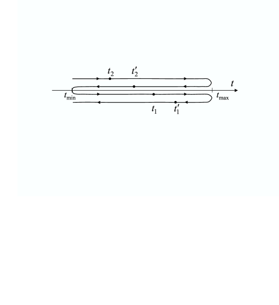
Figure 1: The contour in the complex time which is used to calculate correlations of distribution functions.

Substituting the result (107) into Eq. (A), one finds

$$\langle\delta{\cal F}_{ij}(X_{1},{\bf p}_{1})\>\delta{\cal F}_{kl}(X_{2},{\bf p}_{2})\rangle = 4E_{{\bf p}_{1}}E_{{\bf p}_{2}}\int\frac{dp^{0}_{1}}{2\pi}\,\Theta(p_{1}^{0})\int\frac{dp^{0}_{1}}{2\pi}\,\Theta(p_{2}^{0})\int d^{4}u_{1}\int d^{4}u_{1}\>e^{i(p_{1}u_{1}+p_{2}u_{2})}$$

$$\times i\Delta^{<}_{kj}(X_{2}+\frac{u_{2}}{2},X_{1}-\frac{u_{1}}{2})\;i\Delta^{>}_{il}(X_{1}+\frac{u_{1}}{2},X_{2}-\frac{u_{2}}{2})$$

$$= 4E_{{\bf p}_{1}}E_{{\bf p}_{2}}\int\frac{dp^{0}_{1}}{2\pi}\,\Theta(p_{1}^{0})\int\frac{dp^{0}_{1}}{2\pi}\,\Theta(p_{2}^{0})\int d^{4}u_{1}\int d^{4}u_{1}$$

$$\times \int\frac{d^{4}k_{1}}{(2\pi)^{4}}\int\frac{d^{4}k_{2}}{(2\pi)^{4}}\;e^{i(p_{1}u_{1}+p_{2}u_{2}-k_{1}\tilde{u}_{1}-k_{2}\tilde{u}_{2})}i\Delta^{<}_{kj}(\tilde{X}_{1},k_{1})i\Delta^{>}_{il}(\tilde{X}_{2},k_{2})\;,$$

where

$$\tilde{X}_{1}\equiv\frac{1}{2}(X_{1}+X_{2})-\frac{1}{4}(u_{1}+u_{2})\;,\;\;\;\;\;\tilde{u}_{1}\equiv X_{2}-X_{1}+\frac{1}{2}(u_{1}+u_{2})\;,$$

$$\tilde{X}_{2}\equiv\frac{1}{2}(X_{1}+X_{2})+\frac{1}{4}(u_{1}+u_{2})\;,\;\;\;\;\;\tilde{u}_{2}\equiv X_{1}-X_{2}+\frac{1}{2}(u_{1}+u_{2})\;.$$

And now we adopt the assumption which is crucial for our further considerations. Namely, we assume that the system under consideration is on average homogeneous and stationary. Therefore, the Wigner transformed Green’s functions and the average distribution functions are independent of space-time variable $X,X_{1},X_{2},\tilde{X}_{1}$ or $\tilde{X}_{2}$, respectively. We also assume that the average distrubtion function has the structure $\langle{\cal F}_{ij}(X,{\bf p})\rangle=\delta^{ij}n({\bf p})$. Then, the formulas (100, 101) get the form

$$i\Delta^{<}_{ij}(X,p)=\frac{\pi}{E_{\bf p}}\delta(E_{\bf p}-p^{0})\delta^{ij}n({\bf p})+\frac{\pi}{E_{\bf p}}\delta(E_{\bf p}+p^{0})\delta^{ij}\big{[}\bar{n}(-{\bf p})+1\big{]}\;,$$ (109)

$$i\Delta^{>}_{ij}(X,p)=\frac{\pi}{E_{\bf p}}\delta(E_{\bf p}-p^{0})\delta^{ij}\big{[}n({\bf p})+1\big{]}+\frac{\pi}{E_{\bf p}}\delta(E_{\bf p}+p^{0})\delta^{ij}\bar{n}(-{\bf p})\;.$$ (110)

Substituting the Green’s functions (109, 110) into Eq. (A), the integrals over $p^{0}_{1}$, $p^{0}_{2}$, $u_{1}$ and $u_{2}$ can be trivially performed and one finds

$$\langle\delta{\cal F}_{ij}(X_{1},{\bf p}_{1})\>\delta{\cal F}_{kl}(X_{2},{\bf p}_{2})\rangle = \delta^{il}\delta^{jk}\int\frac{d^{4}k_{1}}{(2\pi)^{4}}\int\frac{d^{4}k_{2}}{(2\pi)^{4}}\frac{E_{{\bf p}_{1}}E_{{\bf p}_{2}}}{E_{{\bf k}_{1}}E_{{\bf k}_{2}}}\;e^{i(k_{1}-k_{2})(X_{1}-X_{2})}$$

$$\times (2\pi)^{4}\delta^{(4)}\Big{(}p_{1}-\frac{k_{1}}{2}-\frac{k_{2}}{2}\Big{)}(2\pi)^{4}\delta^{(4)}\Big{(}p_{2}-\frac{k_{1}}{2}-\frac{k_{2}}{2}\Big{)}n({\bf k}_{1})\big{[}1+n({\bf k}_{2})\big{]}\;.$$

Using the variables $Q\equiv(k_{1}+k_{2})/2$ and $q\equiv k_{1}-k_{2}$, we finally obtain the main result of the Appendix

$$\langle\delta{\cal F}_{ij}(X_{1},{\bf p}_{1})\>\delta{\cal F}_{kl}(X_{2},{\bf p}_{2})\rangle = \delta^{il}\delta^{jk}(2\pi)^{3}\delta^{(3)}({\bf p}_{1}-{\bf p}_{2})$$

$$\times \int\frac{d^{3}q}{(2\pi)^{3}}\frac{E_{{\bf p}_{1}}E_{{\bf p}_{2}}}{E_{{\bf p}_{1}+{\bf q}/2}E_{{\bf p}_{1}-{\bf q}/2}}\;e^{iq(X_{1}-X_{2})}n({\bf p}_{1}+{\bf q}/2)\big{[}1+n({\bf p}_{1}-{\bf q}/2)\big{]}\;,$$

where $q^{0}\equiv E_{{\bf p}_{1}+{\bf q}/2}-E_{{\bf p}_{1}-{\bf q}/2}$. Another derivation of the formula analogous to (A) for particles with no internal degrees of freedom or for particles with spin can be found in Tsytovich89 . In our opinion, however, the decomposition, which corresponds to our Eq. (A), is not very convincing as obtained in Tsytovich89 . Just to justify this step of derivation, we have referred to the Keldysh-Schwinger technique.

One observes that the main contribution to the integral over ${\bf q}$ in Eq. (A) comes from such ${\bf q}$ that $|{\bf q}|\leq 1/|{\bf X}_{1}-{\bf X}_{2}|$. If the characteristic (momentum) scale at which the distribution function $n({\bf p})$ changes sizably (for the equilibrium gas of massless particles the scale is given by the gas temperature ($T$)) is much bigger than $1/|{\bf X}_{1}-{\bf X}_{2}|$ (for the equilibrium gas we require $1\ll|{\bf X}_{1}-{\bf X}_{2}|T$)), the function under the integral can be approximated assuming that $|{\bf q}|\ll|{\bf p}_{1}|$. Then, $q^{0}={\bf v}_{1}{\bf q}$ and one finds the classical correlation function

$$\langle\delta{\cal F}_{ij}(X_{1},{\bf p}_{1})\>\delta{\cal F}_{kl}(X_{2},{\bf p}_{2})\rangle = \delta^{il}\delta^{jk}(2\pi)^{3}\delta^{(3)}({\bf p}_{1}-{\bf p}_{2})\;\delta^{(3)}({\bf X}_{1}-{\bf X}_{2}-{\bf v}_{1}(t_{1}-t_{2}))\;n({\bf p}_{1})\;,$$ (112)

where we have additionally assumed that populations of the system’s modes are small ($n({\bf p}_{1})\ll 1$). Eq. (112), as well as Eq. (A), is valid for both equilibrium and nonequilibrium systems.

References

(1)
St. Mrówczyński,
Acta Phys. Polon. B 37, 427 (2006).
(2)
M. Asakawa, S. A. Bass and B. Muller,
Prog. Theor. Phys. 116, 725 (2007).
(3)
P. Arnold, G. D. Moore and L. G. Yaffe,
Phys. Rev. D 72, 054003 (2005).
(4)
P. Arnold and G. D. Moore,
Phys. Rev. D 73, 025006 (2006).
(5)
A. Rebhan, P. Romatschke and M. Strickland,
JHEP 0509, 041 (2005).
(6)
A. Dumitru, Y. Nara and M. Strickland,
Phys. Rev. D 75, 025016 (2007).
(7)
P. Romatschke and R. Venugopalan,
Phys. Rev. D 74, 045011 (2006).
(8)
D. Bodeker and K. Rummukainen,
JHEP 0707, 022 (2007).
(9)
J. Berges, S. Scheffler and D. Sexty,
Phys. Rev. D 77, 034504 (2008).
(10) A.I. Akhiezer, I.A. Akhiezer, R.V. Polovin, A.G. Sitenko,
and K.N. Stepanov, Plasma Electrodynamics (Pergamon, New York, 1975).
(11) A.G. Sitenko, Fluctuations and Non-Linear Wave
Interactions in Plasmas, (Pergamon, Oxford, 1982).
(12) H.D. Sivak, Ann. Phys. (N.Y.) 159, 351 (1985).