Molecular cloud abundances and anomalous diffusion

Abstract

The chemistry of molecular clouds has been studied for decades, with an increasingly general and sophisticated treatment of the reactions involved. Yet the treatment of turbulent diffusion has remained extremely sketchy, assuming simple Fickian diffusion with a scalar diffusivity $D$. However, turbulent flows similar to those in the interstellar medium are known to give rise to anomalous diffusion phenomena, more specifically superdiffusion (increase of the diffusivity with the spatial scales involved). This paper considers to what extent and in what sense superdiffusion modifies molecular abundances in interstellar clouds. For this first exploration of the subject we employ a very rough treatment of the chemistry and the effect of non-unifom cloud density on the diffusion equation is also treated in a simplified way. The results nevertheless clearly demonstrate that the effect of superdiffusion is quite significant, abundance values at a given radius being modified by order of unity factors. The sense and character of this influence is highly nontrivial.

1 Introduction

The chemistry of molecular clouds is a complex system affected by different factors. The first models laid down the foundations of the chemical reaction network: following the initial steady state gas-phase chemistry model of Herbst & Klemperer (1973) several (pseudo-)time-dependent models, with fixed profiles of physical parameters were developed, considering more and more chemical reactions, while neglecting photodissociation (Leung et al. 1984; Herbst & Leung 1989; Millar & Herbst 1990). The agreement of the models with observed fractional abundances improved when the effect of turbulent diffusion was taken into account, resulting in smoother density distribution profiles for the more important species (Xie et al. 1995, hereafter XAL95). Subsequent models further refined the chemistry, considering details of the ion-neutral reaction scheme, and taking into account the gas-grains interaction, $\mathrm{H_{2}}$ and CO self-shielding, grain accretion effects and adsorption onto grains (Willacy et al. 2002; Yate & Millar 2003).

In contrast to the enormous efforts made in order to improve the representation of chemical processes, the treatment of turbulent diffusion has remained extremely sketchy, assuming simple Fickian diffusion with a scalar diffusivity $D$. Under the conditions prevailing in interstellar space this is surely wrong. Interstellar turbulence is mainly driven by supernova shocks on spatial scales far exceeding that of the molecular clouds. From those scales, kinetic energy cascades down to the scale of clouds, cloud clumps and even cloud cores (Boldyrev 2002; Scalo & Elmegreen 2004; Ryan Joung et al. 2006). Indeed, in current thinking clouds are hardly more than positive density fluctuations in this large-scale compressible turbulent flow. In such a turbulent flow, the increase of the r.m.s. separation $\Delta$ of two tracer particles will only be due to eddies smaller than $\Delta$, leading to a scale-dependent eddy diffusivity. As a result, the increase of $\Delta$ with time will deviate from the Fickian square-root law: such non-Fickian or anomalous diffusive processes commonly occur in various fields of physics (Avellaneda & Majda 1992), though astrophysical applications have so far been limited to solar physics (Petrovay 1999). As in the turbulent cascade the diffusivity increases for larger spatial scales, the transport of passive scalars by inertial-range turbulence belongs to the subclass of superdiffusive processes.

The work presented here is a first exploration of the effect of superdiffusion on the chemistry of molecular clouds. Our approach is described in Section 2. In order to get a first impression of the importance of superdiffusive effects, we neglect the intricacies of the chemical reaction network and treat their net effect as a simple parametric source term in the diffusion equation. As anomalous diffusivity cannot be described by any partial differential equation in physical space, we are forced to work in Fourier space, with $D=D(k)$ a function of the wavenumber $k$. To alleviate the ensuing difficulties, in Section 3.1 we first consider a case where the density of the main component is uniform throughout the cloud. A semianalytical solution is possible in this case; the results indicate that there are significant and nontrivial differences between the diffusive and superdiffusive cases. Section 3.2 then considers what changes are to be expected if the assumption of a uniform cloud is dropped. Section 4 concludes the paper.

2 Formulation of the problem

Consider a spherically symmetric molecular cloud, with $r$ the radial coordinate. Let $n_{\mathrm{\scriptsize H_{2}}}(r)$ denote the number density of hydrogen, $n_{i}(r,t)$ the number density and $f_{i}={n_{i}\over n_{H_{2}}}$ the fractional abundance of a tracer molecule $i$. On the basis of simple mixing-length arguments (cf. XAL95), if turbulence is characterized by a single dominant scale $l$ and velocity $v$, the diffusion equation for the tracer reads

$$\partial_{t}n_{i}(r,t) = D\nabla[\nabla n_{i}(r,t)-f_{i}(r,t)\nabla n_{\mathrm{\scriptsize H_{2}}}(r)]$$

$$+S_{i}(r,t),$$

where $S_{i}(r,t)$ is the source/sink term, representing the chemistry reaction scheme, and $D=\langle lv\rangle$ is the diffusion coefficient. In previous work the fiducial values $v\sim 1\,$km/s and $l\sim 0.1$ pc were used, yielding diffusivities on the order of $10^{22}$–$10^{23}\,$cm²/s.

As here we focus on the diffusive term, the chemical source term will be represented very roughly as a simple relaxation term

$$S(r,t)=\frac{n_{0}(r)-n(r,t)}{\tau_{c}}$$ (2)

throughout this paper. Here $n_{0}(r)$ is the diffusionless equilibrium solution, while $\tau_{c}$ is a relaxation timescale on which the solution would converge to $n_{0}(r)$, were there no diffusive effects. On the basis of the results presented in XAL95 the value of $\tau_{c}$ can be estimated to lie in the range $10^{5}$–$10^{6}$ years.

!t

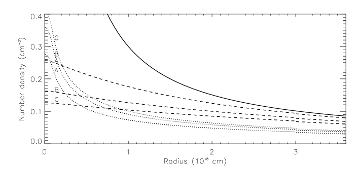
Figure 1: Number density as a function of the radius in a uniform density cloud for a tracer whose distribution scales as $n_{0}\sim 1/r$ in the nondiffusive case (solid line). Dashed line: normal diffusive case; dotted line: superdiffusive case. The parameters are: $\mathrm{\tau_{c}=10^{6}yrs}$, and D = $\mathrm{4\times 10^{22}}$ (A); $\mathrm{10^{23}}$ (B); $\mathrm{D=1.6\times 10^{23}cm^{2}s^{-1}}$ (C).

!t

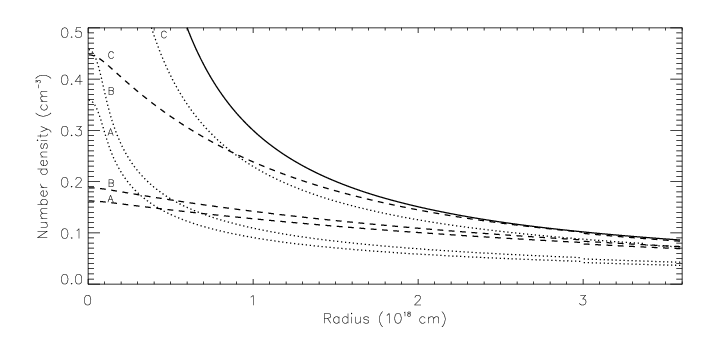
Figure 2: Same as in Fig. 1. but the parameters are: $\mathrm{D=10^{23}cm^{2}s^{-1}}$, and $\mathrm{\tau_{c}}$ = $\mathrm{10^{6}}$ (A); $\mathrm{7.6\times 10^{5}}$ (B); $\mathrm{1.2\times 10^{5}yrs}$ (C).

!t

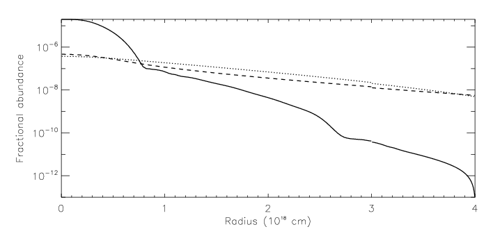
Figure 3: Fractional abundance of ${\mathrm{O_{2}}}$ as a function of radius in a uniform density cloud, with $D=10^{23}\,$cm${}^{2}/$s, $\tau_{c}=10^{6}$ yrs. Solid line: nondiffusive case, adopted from XAL95. Dashed line: normal diffusive case; dotted line: superdiffusive case.

In a turbulent cascade regime where turbulence cannot be characterized by a single dominant scale anymore, equation (1) does not hold. However, its Fourier transform, with the appropriate scale-dependent diffusivity value $D(k)$ will still hold for each Fourier component of the passive scalar field. For the wavenumber dependence of the diffusivity we use the Kolmogorov form $D(k)=D_{0}(k/k_{0})^{-4/3}$ throughout this paper, $D_{0}$ being the value of the diffusivity at the wavenumber $k_{0}$, corresponding to the fiducial scale $l$ used in previous work.

3 Results

3.1 Uniform density cloud

The Fourier transform of equation (1) takes a particularly simple form if the main constituent (i.e. H₂) is distributed uniformly. Equation (1) then simplifies to

$$\partial_{t}n(r,t)=D\nabla^{2}n(r,t)+S(r,t)$$ (3)

The spatial Fourier transform of this is

$$\partial_{t}\hat{n}(k,t)=-D(k)k^{2}\hat{n}(k,t)+\hat{S}(k,t)$$ (4)

In the stationary case the solution is

$$\hat{n}(k,t)={\hat{n}_{0}(k,t)\over 1+\tau_{c}D(k)k^{2}}.$$ (5)

Transforming $\hat{n}(k,t)$ back to physical space we obtain the equilibrium distribution of the tracer.

To carry out these transforms in the spherical geometry at hand, we recall the theorem that an $n$ dimensional Fourier transform can be replaced a one dimensional Hankel transform, if the transformable function depends only on $r=\sqrt{\sum{}x_{i}^{2}}$ (Sneddon 1951). In three dimensions the transformation formulae are:

$$\hat{n}(k)=\int_{0}^{\infty}{r^{3\over 2}n(r)J_{1\over 2}(kr)dr}$$ (6)

$$n(r)=\int_{0}^{\infty}{k^{3\over 2}\hat{n}(k)J_{1\over 2}(kr)dk}.$$ (7)

where $J_{1\over 2}$ is the Bessel function of order $\frac{1}{2}$. These Hankel transforms can only be computed analytically for some special cases, such as a Gaussian profile for $n_{0}(r)$ (cf. Marschalkó 2006). For the more realistic cases presented below, equations (6) and (7) were evaluated numerically.

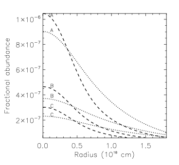
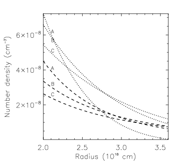
Figure 4: Same as in Fig. 3. but the inner and outer parts of the cloud are shown separately. The values of parameters are: $\mathrm{\tau_{c}=10^{6}yrs}$, D = $\mathrm{4\times 10^{22}}$ (A), $\mathrm{10^{23}}$ (B) and $\mathrm{D=1.6\times 10^{23}cm^{2}s^{-1}}$ (C).

In figures 1 and 2 we present analytical solutions assuming $n_{0}(r)\sim r^{-1}$, a very rough analytical approximation for the actual profiles. It is apparent that there is a significant difference between the diffusive and superdiffusive case. In the superdiffusive case the concentration of the tracer in the cloud core is much more pronounced, as a consequence of the reduced diffusivity at small scales. Interestingly, an overall increase of the diffusivity $D$ leads to an increase in the central number density of the tracer in the diffusive case, while it leads to a decrease in the superdiffusive case (though this trend reverses at large values of $r$).

Next, instead of the generic $1/r$ distribution we consider one particular tracer, the oxygen molecule. The form of $n_{0}(r)$ for this molecule is taken from XAL95. Figure 3 shows the fractional abundance of O₂ as a function of the radius, still assuming a uniform H₂ distribution. The diffusive and superdiffusive cases are again significantly different, but this distinction is better seen in the non-logarithmic plot (Figure 4). In contrast to the $1/r$ case with its singular chemical source function, in the superdiffusive solutions the tracer is now less concentrated to the core than with Fickian diffusion.

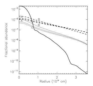
Figure 5: Comparison of the O₂ fractional abundance profiles computed assuming normal (Fickian) diffusion with uniform (dotted) and non-uniform (dashed) cloud density. Case A: $D=10^{23}\,$cm²/s, $\tau_{c}=7.6\times 10^{5}$ yrs. Case B: $D=4\times 10^{22}\,$cm²/s, $\tau_{c}=10^{6}$ yrs. Case C: $D=10^{23}\,$cm²/s, $\tau_{c}=10^{6}$ yrs. Solid: initial profile $n_{0}(r)$.

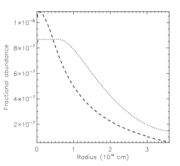
Figure 6: Fractional abundance of O₂ as a function of radius in a cloud of non-uniform density, with $D=10^{23}\,$cm²/s, $\tau_{c}=7.6\times 10^{5}$ yrs. Dashed line: normal diffusion. Dotted line: the expected abundance profile with superdiffusion, obtained by the rescaling method described in the text.

3.2 Non-uniform cloud

The non-uniformity of the cloud was in fact implicitly already taken into account in the previous subsection, as $n_{0}(r)$ was taken from non-uniform cloud models. To make our approach more consistent, it would be necessary to take into account this non-uniformity also explicitly in equation (1). In this more general case the problem becomes mathematically much more complicated. In order to get a first impression of the importance of the inhomogeneity, here we first compare the results obtained with and without explicitly treating non-uniformity for the case of normal diffusion. For these calculations the density profile $n_{\mathrm{\scriptsize H_{2}}}(r)$ was taken from XAL95, as above.

For the solution of equation (1) a time-relaxation method was used with a finite difference scheme first order accurate in time and second order accurate in space, on a grid of 512 points evenly distributed between $r_{\mathrm{\scriptsize{in}}}=4\times 10^{15}$ and $r_{\mathrm{\scriptsize{out}}}=4\times 10^{18}\,$cm. At the inner boundary of our domain the boundary condition was $\partial_{r}n(r=r_{\mathrm{\scriptsize{in}}},t)=0$, while at the outer boundary the number density was set to zero $n(r=r_{\mathrm{\scriptsize{out}}},t)=0$. Starting from the same initial conditions as in the previous case, the solution was allowed to evolve in time. Comparing the solutions obtained in the uniform case to the exact stationary solution obtained from equation (5) we found that satisfactory agreement is reached within one characteristic time $\tau_{c}$.

The results are plotted in figure 5. The effect of non-uniformity is clearly to increase the tracer abundance, especially in the outer parts of the cloud. Nevertheless, varying the parameters of the problem ($D_{0}$, $\tau_{c}$) the resulting effects are qualitatively similar and quantitatively comparable to those found in the uniform case. This encourages us to attempt to characterize the effect of superdiffusion in the nonuniform case by rescaling the uniform superdiffusive solution for the fractional abundance (dotted line in figure 3) by the ratio of the nonuniform and uniform solutions in the normal diffusive case. The resulting abundance curve is plotted in figure 6. Just as in the uniform case (figure 3), superdiffusion reduces the O₂ abundance in the cloud core and increases it in the envelope.

4 Conclusion

In this paper we considered to what extent and in what sense superdiffusion modifies molecular abundances in interstellar clouds. The results clearly demonstrate that the effect is quite significant, abundance values at a given radius being modified by order of unity factors. The sense and character of this influence is highly nontrivial.

In order to make a meaningful comparison with observational data possible, this model needs to be developed further to include a realistic treatment of the chemical reactions and to include a more rigorous calculation of the effect of non-uniformity of the cloud in the diffusion equation. Work in this direction is in progress.

- [1] Avellaneda, M., Majda, A.J.: 1992, Phys. Fluids A 4, 41
- [2] Boldyrev, S.: 2002, ApJ 569, 841
- [3] Herbst, E., Klemperer, W.: 1973, ApJ 185, 505
- [4] Herbst, E., Leung, C.M.: 1989, ApJS 69, 271
- [5] Leung, C.M., Herbst, E., Heubner. W. F.: 1984, ApJS 56, 231
- [6] Marschalkó, G.: 2006, PADEU 17, 179
- [7] Millar, T.J., Herbst, E.: 1990, A&A 231, 466
- [8] Petrovay, K.: 1999, SSRv. 95, 9
- [9] Ryan Joung, M.K., Mac Low, M.: 2006, ApJ 653, 1266
- [10] Scalo, J., Elmegreen, B.G.: 2004, ARA&A 42, 275
- [11] Sneddon, I. N.: 1951, Fourier transforms (McGraw-Hill, New York), p.62
- [12] Willacy, K., Langer, W.D., Allen. M.: 2002, ApJ 573, L119
- [13] Xie, T., Allen. M., Langer, W.D.: 1995, ApJ 440, 674 (XAL95)
- [14] Yate, C.J., Millar, T.J.: 2003, A&A 399, 553