Atomic teleportation via cavity QED and position measurements: efficiency analysis

Abstract

We have recently presented a novel protocol to teleport an unknown atomic state via cavity QED and position measurements. Here, after a brief review of our scheme, we provide a quantitative study of its efficiency. This is accomplished by an explicit description of the measurement process that allows us to derive the fidelity with respect to the atomic internal state to be teleported.

I Introduction

The key role played by quantum entanglement in a number of crucial quantum information processing tasks is now firmly grounded nc . One of the most striking applications harnessing such powerful resource is the teleportation of an unknown qubit, the unit of quantum information, between two distant systems first proposed in famous paper by Bennett et al. bennett . The idea is essentially to transfer an unknown quantum state from an input qubit $A$ to a target qubit $B$ by using an ancilla, e.g. a third auxiliary qubit $C$. Teleportation is achieved via preparation of initial maximally entangled states between qubits $B$ and $C$ and successive Bell measurements on $A$ and $C$. This phenomenon soon obtained large attention especially after in its experimental demonstrations bowm-boschi ; NMR ; natphys ; nature .

Of course, due to its purely quantum nature, teleportation can be attained in systems that exhibit a fully quantum behaviour. This is one of the reasons why cavity quantum electrodynamics (QED), where coherent coupling between Rydberg atoms and the quantized electromagnetic (e.m.) field is possible raimond , has been soon addressed as a promising scenario to achieve teleportation teleportation-QED . In cavity-QED schemes for teleporting states between two atoms, the typical strategy is indeed to harness the coherent atom-field interaction using cavity e.m. modes and/or additional atoms as ancillary systems.

Among these works are some recent schemes where direct (in general quite difficult) projections onto Bell states are avoided vaidman ; de-almeida ; zheng ; ye-guo ; cardoso . In particular, Zheng has proposed a scheme for approximately teleporting an unknown internal state between two atoms which successively interact with a cavity mode according to the Jaynes-Cummings Hamiltonian zheng . Ye and Guo have presented another scheme that does not require projections onto Bell-state and makes use of three atoms and a single-mode cavity field out of resonance ye-guo . The atom-atom coupling via the virtual excitations of the cavity field is exploited for teleporting a quantum state between two atoms. The probability of success of the Zheng scheme is 1/4, whereas the teleportation is successful with probability 1/2 in the proposal by Ye and Guo. Noticeably, both the schemes require precise tuning of the atom-cavity field interaction time zheng ; ye-guo .

Very recently, we have proposed the first cavity-QED scheme that exploits the atomic translational dynamics in order to accomplish teleportation between two atoms TC . Among the major advantages are the probability of success of 1/2, the need to measure only product states as well as the ability of the protocol to work without any holonomous constraint on the atom-photon interaction times. In particular, the latter feature implies that, unlike other schemes zheng ; ye-guo no precise tuning of the atom-cavity field interaction times is required. It only suffices that such times are large enough in order for which-path information of the two atoms to become accessible.

In Ref. TC , we have provided evidence that position measurements enable successful teleportation in the regime of accessible which-path information. This phenomenon was shown to stem from the asymptotic orthogonality of the field-deflected atomic wavepackets Vag-Cus ; which-path . In this work, we make such conclusions more exact by explicitly including the measurement process of the atomic positions. This allows us to calculate the fidelity with respect to the state to be teleported as a function of the parameters entering the dynamics. We derive a lower bound for such a quantity and study its dependence on the measured atomic positions and the atom-cavity interaction times.

This paper is organized as follows. In Sec. II, we introduce the system and the Hamiltonian. In Sec. III, we review the teleportation scheme of Ref. TC . In Sec. IV, we calculate the final state of the atom-field system once all the necessary measurements required for successful teleportation have been explicitly taken into account. In Sec. V we analyze the efficiency of the scheme in terms of the fidelity with respect to the atomic state to be teleported. We also provide a lower bound for such a quantity and investigate its behaviour as a function of the measured atomic positions and the atom-field interaction times. Finally, in Sec. VI we draw our conclusions.

II System and approach

We consider two identical two-level atoms, labeled 1 and 2, of mass $m$ and Bohr frequency $\omega$. The atoms interact in succession with the e.m. field of the same e.m. cavity. We assume that the velocity of each atom along the $z$-direction (orthogonal to the $x$-cavity axis) is large enough that the motion along the $z$-axis is not affected by the cavity field and can be treated classically. Denoting by $a$ and $a^{{\dagger}}$ the annihilation and creation operators of the cavity field and assuming the resonance condition, the free Hamiltonian $H_{0}$ can be written as

$$H_{0}=\sum_{i=1,2}\left[\frac{\hat{p}_{i}^{2}}{2m}+\hbar\omega S_{z,i}\right]+\hbar\omega a^{{\dagger}}a\,,$$ (1)

where – for each atom $i=1,2$ – $S_{z,i},S_{\pm,i}$ are the usual spin-1/2 operators and $\hat{p}_{i}=-i\hbar(d/dx_{i})$ is the $x$-component of the momentum operator. In the Rotating Wave Approximation, each atom $i$ couples to the cavity field according to the interaction Hamiltonian

$$H_{if}=\hbar\varepsilon\sin(k\hat{x}_{i})\left(a^{{\dagger}}S_{-,i}+aS_{+,i}\right)\,\,\,\,(i=1,2)$$ (2)

with $k$ and $\varepsilon$ standing for the wave number of the e.m. mode and the atom-field coupling constant, respectively, and where $\hat{x}_{i}$ is the $i$th atomic position operator along the cavity axis.

Hamiltonian (2) accounts for the spatial structure of the e.m. field along the $x$-cavity axis. Based on such Hamiltonian model, a number of observable phenomena have been shown such as the optical Stern-Gerlach effect SGE , self-induced transparency schlicher , modulation of the atomic decay in a damped cavity wilkens and non-dissipative damping of the Rabi oscillations Vag-Cus ; which-path .

When both the atomic wavepackets have width $\sigma_{x_{i}}$ small enough compared with the cavity wavelength $2\pi/k$ ($\sigma_{x_{i}}\ll 2\pi/k$) and in a nodal region of the cavity $H_{i}$, can be approximated as nota-nodale

$$H_{iN} = \hbar\varepsilon k\,\hat{x}_{i}\left(a^{{\dagger}}S_{-,i}+aS_{+,i}\right),$$ (3)

where $\hat{x}_{i}$ stands for the atomic position operator of the $i$th atom with respect to the nodal point.

At time $t=0$, atom 1 enters the cavity and interacts with the field for a time $t_{1}$. At a later time $t_{2}>t_{1}$, atom 2 enters the cavity and couples to the field state modified by the first atom. At time $t_{3}>t_{2}$ atom 2 exits the cavity. At times $t\geq t_{3}$ both the atoms are therefore out of the cavity and evolve freely. In the interaction picture, the Hamiltonian at all times reads

$$H_{N}^{I}(t) = \hbar\varepsilon k\left(\hat{x}_{1}+\frac{\hat{p}_{1}}{m}t\right)\mu_{t}(0,t_{1})u_{1}+\hbar\varepsilon k\left(\hat{x}_{2}+\frac{\hat{p}_{2}}{m}t\right)\mu_{t}(t_{2},t_{3})u_{2}\,,$$ (4)

where we have introduced the atom-field operators $u_{i}=a^{{\dagger}}S_{-,i}+aS_{+,i}$ and where the time interval during which each atom interacts with the cavity mode is accounted for by means of the function $\mu_{t}(t^{\prime},t^{\prime\prime})=\theta(t-t^{\prime})-\theta(t-t^{\prime\prime})$, $\theta(t)$ being the usual Heaviside function. Of course, in the time interval $[t_{1},t_{2}]$ and for $t\geq t_{3}$ $H_{N}^{I}(t)$ vanishes since no atom is inside the cavity. The Hamiltonian operator of Eq. (4) can be used to derive the exact dynamics of a given initial state of the two-atom-field system at times $t\geq t_{3}$ through the respective evolution operator $U_{N}^{I}(t\geq t_{3})$

$$U_{N}^{I}(t\geq t_{3})=T\,\exp\left[-\frac{i}{\hbar}\int_{0}^{t_{3}}H_{N}^{I}(t)dt\right]$$ (5)

with $T$ standing for the time-ordering operator and where the second integration bound is due to the fact that $H_{N}^{I}=0$ for $t\geq t_{3}$.

Due to the fact that atom 2 enters the cavity after atom 1 has come out of it, it is possible to split up $U_{N}^{I}(t\geq t_{3})$ into the product of two evolution operators $U_{N,1}^{I}(t\geq t_{3})$ and $U_{N,2}^{I}(t\geq t_{3})$. Each operator $U_{N,i}^{I}(t\geq t_{3})$ only affects the dynamics of atom $i$. In formulae (from now on, whenever unnecessary, the time argument “$(t\geq t_{3})$” and/or the apex “$I$” in the evolution operators will be omitted)

$$U_{N}=U_{N,2}\cdot U_{N,1}$$ (6)

with

$$U_{N,1}=T\,\exp\left[-\frac{i}{\hbar}\int_{0}^{t_{1}}H_{N}^{I}(t)dt\right]=U_{N,1}(\hat{x}_{1},\hat{p}_{1},u_{1}),$$ (7)

$$U_{N,2}=T\,\exp\left[-\frac{i}{\hbar}\int_{t_{2}}^{t_{3}}H_{N}^{I}(t)dt\right]=U_{N,2}(\hat{x}_{2},\hat{p}_{2},u_{2}),$$ (8)

where in the right-hand side of both equations we have explicitly indicated the quantities the $U_{N,i}$’s depends on according to Eq. (4).

III Teleportation scheme

We denote the ground and excited states of the $i$th atom by $\left|g_{i}\right\rangle$ and $\left|e_{i}\right\rangle$, respectively. Assume that atom 2 is the one whose initial internal state, say $\left|\alpha\right\rangle_{2}$, is to be teleported. Such state is written as

$$\left|\alpha\right\rangle_{2}=\cos\frac{\vartheta}{2}\left|e_{2}\right\rangle+e^{i\varphi}\sin\frac{\vartheta}{2}\left|g_{2}\right\rangle$$ (9)

with $\vartheta\in[0,\pi]$ and $\varphi\in[0,\pi]$.

By indicating the Fock states of the cavity field as $\left|n\right\rangle$ ($n=0,1,...$), we consider the initial state of the system $\left|\Psi(0)\right\rangle=\left|\varphi_{1}(0)\right\rangle\left|e_{1}\right\rangle\,\,\left|\varphi_{2}(0)\right\rangle\left|\alpha\right\rangle_{2}\,\,\left|0\right\rangle$ where $\left|\varphi_{i}(0)\right\rangle$ (associated with each atom $i=1,2$) is a Gaussian wavepacket of minimum uncertainty, such that the product between the initial position and momentum widths fulfills $\sigma_{x_{i}}\cdot\sigma_{p_{i}}=\hbar/2$. Consider now the usual dressed states of the $i$th atom $\left|\chi_{n,i}^{\pm}\right\rangle=\left(\left|e_{i}\right\rangle\left|n\right\rangle\pm\left|g_{i}\right\rangle\left|n+1\right\rangle\right)/\sqrt{2}$ ($n=0,1,...$). These states are eigenstates of the $u_{i}$ operators since $u_{i}\left|\chi_{n,i}^{\pm}\right\rangle=\pm\sqrt{n+1}\left|\chi_{n,i}^{\pm}\right\rangle$ (while $u_{i}\left|g_{i}\right\rangle\left|0\right\rangle=0$). The dressed states together with $\left|g_{i}\right\rangle\left|0\right\rangle$ ($i=1,2$) represent an orthonormal basis of the corresponding Hilbert space. As $u_{i}$ commutes with $U_{N,i}$ according to Eqs. (4), (7) and (8), the effective representation $U_{N,i}^{(n,\pm)}$ of $U_{N,i}$, as applied to a dressed state $\left|\chi_{n,i}^{\pm}\right\rangle$, is obtained by simply replacing $u_{i}$ with $\pm\sqrt{n+1}$ in Eqs. (7) and (8). This yields

$$U_{N,i}^{(n,\pm)}=U_{N,i}(\hat{x}_{i},\hat{p}_{i},\pm\sqrt{n+1})\,\,\,\,\,\,\,(n=0,1,...),$$ (10)

while the effective representation of $U_{N,i}$ – as applied to state $\left|g_{i}\right\rangle\left|0\right\rangle$ – reduces to the identity operator for both the atoms $i=1,2$. The operators in Eq. (10) clearly affects only the atomic translational dynamics and therefore allows to define a family of atomic translational wavepackets $\left|\Phi_{n,i}^{\pm}\right\rangle$ according to $\left|\Phi_{n,i}^{\pm}\right\rangle=U_{N,i}^{(n,\pm)}\left|\varphi_{i}(0)\right\rangle$ such that

$$U_{N,i}\left|\varphi_{i}(0)\right\rangle\left|\chi_{n,i}^{\pm}\right\rangle=\left|\Phi_{n,i}^{\pm}\right\rangle\left|\chi_{n,i}^{\pm}\right\rangle.$$ (11)

Once the time evolution operator (6) is applied to the initial state $\left|\Psi(0)\right\rangle$, the state of the whole system at a time $t\geq t_{3}$ – when both the atoms are out of the cavity – can be written in the form

$$\left|\psi(t_{3})\right\rangle=\left|\lambda_{0,1}\right\rangle\left|\varphi_{2}(0)\right\rangle\left|g_{2}\right\rangle\left|0\right\rangle+\sum_{n=0,1}\sum_{\eta=-,+}\left(\left|\lambda_{n,1}^{\eta}\right\rangle\left|\Phi_{n,2}^{\eta}\right\rangle\left|\chi_{n,2}^{\eta}\right\rangle\right),$$

where the $\lambda$ states of atom 1 are defined according to

$$\left|\lambda_{0,1}\right\rangle = \left(\frac{\left|\Phi_{0,1}^{+}\right\rangle+\left|\Phi_{0,1}^{-}\right\rangle}{2}\right)\,e^{i\varphi}\sin\frac{\vartheta}{2}\left|e_{1}\right\rangle,$$ (12)

$$\left|\lambda_{0,1}^{\pm}\right\rangle = \left(\frac{\left|\Phi_{0,1}^{+}\right\rangle+\left|\Phi_{0,1}^{-}\right\rangle}{2\sqrt{2}}\right)\,\cos\frac{\vartheta}{2}\left|e_{1}\right\rangle\pm\left(\frac{\left|\Phi_{0,1}^{+}\right\rangle-\left|\Phi_{0,1}^{-}\right\rangle}{2\sqrt{2}}\right)\,e^{i\varphi}\sin\frac{\vartheta}{2}\left|g_{1}\right\rangle,$$ (13)

$$\left|\lambda_{1,1}^{\pm}\right\rangle = \left(\frac{\left|\Phi_{0,1}^{+}\right\rangle-\left|\Phi_{0,1}^{-}\right\rangle}{2\sqrt{2}}\right)\cos\frac{\vartheta}{2}\left|g_{1}\right\rangle.$$ (14)

By indicating the time spent inside the cavity by atoms 1 and 2 with $\tau_{1}=t_{2}-t_{1}$ and $\tau_{2}=t_{3}-t_{2}$, respectively, the states $\left|\Phi_{n,i}^{\pm}\right\rangle$ appearing in Eq. (III) fulfill the following important property which-path ; epl-2atoms ; epjd

$$\lim_{\tau_{i}\rightarrow\infty}\left\langle\Phi_{n,i}^{+}\right|\Phi_{n,i}^{-}\rangle=0.$$ (15)

According to Eq. (15), wavepackets $\left|\Phi_{n,i}^{+}\right\rangle$ and $\left|\Phi_{n,i}^{-}\right\rangle$ exhibit a negligible overlap for long enough times of flight $\tau_{i}$. Times of flight of the order of a few Rabi oscillations are sufficient in order to get negligible overlapping epl-2atoms ; epjd . Such noticeable circumstance allows to distinguish the elements of the set of translational states {$\left|\Phi_{n,i}^{\pm}\right\rangle$} through measurements of the atomic positions along the $x$-axis. As can be shown, Eq. (15) yields that all the terms appearing in (III) are mutually orthogonal provided $\tau_{1}$ and $\tau_{2}$ are sufficiently large. By expressing the dressed states $\left|\chi_{n,2}^{\pm}\right\rangle$ appearing in Eq. (III) in terms of states $\left|g_{2}\right\rangle\left|n\right\rangle$ and $\left|e_{2}\right\rangle\left|n\right\rangle$, one recognizes the occurrence of cases where measurements of the photon number, of the internal state of atom 2 and of the positions of the two atoms can make atom 1 collapse into the initial internal state of atom 2 ($\left|\alpha\right\rangle_{2}$), i.e. a successful teleportation can take place.

$\mathbf{\left|n\right\rangle}$	Int. 2	Tr. 1	Tr. 2	Result	Int. 1	$\mathbf{P_{fail}}$
2	–	–	–	Unsuccessful	–	$\frac{1}{8}(1+\cos\vartheta)$
	$\left|e_{2}\right\rangle$	–	–	Unsuccessful	–	$\frac{1}{8}(1+\cos\vartheta)$
	$\left|g_{2}\right\rangle$	$\left|\Phi_{0,1}^{-}\right\rangle$	$\left|\Phi_{0,2}^{-}\right\rangle$	Successful	$\cos\frac{\vartheta}{2}\left|e_{1}\right\rangle+e^{i\varphi}\sin\frac{\vartheta}{2}\left|g_{1}\right\rangle$	–
1	$\left|g_{2}\right\rangle$	$\left|\Phi_{0,1}^{-}\right\rangle$	$\left|\Phi_{0,2}^{+}\right\rangle$	Successful footnote	$\cos\frac{\vartheta}{2}\left|e_{1}\right\rangle-e^{i\varphi}\sin\frac{\vartheta}{2}\left|g_{1}\right\rangle$	–
	$\left|g_{2}\right\rangle$	$\left|\Phi_{0,1}^{+}\right\rangle$	$\left|\Phi_{0,2}^{+}\right\rangle$	Successful	$\cos\frac{\vartheta}{2}\left|e_{1}\right\rangle+e^{i\varphi}\sin\frac{\vartheta}{2}\left|g_{1}\right\rangle$	–
	$\left|g_{2}\right\rangle$	$\left|\Phi_{0,1}^{+}\right\rangle$	$\left|\Phi_{0,2}^{-}\right\rangle$	Successful footnote	$\cos\frac{\vartheta}{2}\left|e_{1}\right\rangle-e^{i\varphi}\sin\frac{\vartheta}{2}\left|g_{1}\right\rangle$	–
	$\left|g_{2}\right\rangle$	–	–	Unsuccessful	–	$\frac{1}{4}(1-\cos\vartheta)$
	$\left|e_{2}\right\rangle$	$\left|\Phi_{0,1}^{-}\right\rangle$	$\left|\Phi_{0,2}^{-}\right\rangle$	Successful	$\cos\frac{\vartheta}{2}\left|e_{1}\right\rangle+e^{i\varphi}\sin\frac{\vartheta}{2}\left|g_{1}\right\rangle$	–
0	$\left|e_{2}\right\rangle$	$\left|\Phi_{0,1}^{-}\right\rangle$	$\left|\Phi_{0,2}^{+}\right\rangle$	Successful footnote	$\cos\frac{\vartheta}{2}\left|e_{1}\right\rangle-e^{i\varphi}\sin\frac{\vartheta}{2}\left|g_{1}\right\rangle$	–
	$\left|e_{2}\right\rangle$	$\left|\Phi_{0,1}^{+}\right\rangle$	$\left|\Phi_{0,2}^{+}\right\rangle$	Successful	$\cos\frac{\vartheta}{2}\left|e_{1}\right\rangle+e^{i\varphi}\sin\frac{\vartheta}{2}\left|g_{1}\right\rangle$	–
	$\left|e_{2}\right\rangle$	$\left|\Phi_{0,1}^{+}\right\rangle$	$\left|\Phi_{0,2}^{-}\right\rangle$	Successful footnote	$\cos\frac{\vartheta}{2}\left|e_{1}\right\rangle-e^{i\varphi}\sin\frac{\vartheta}{2}\left|g_{1}\right\rangle$	–

Table 1: Teleportation measurement scheme. Each case is represented by given outcomes of the number of photons (1^st column), the internal state of atom 2 (2^nd column) and the deflected wavepackets (3^th and 4^th columns). In the 5^th column it is indicated whether or not teleportation has been successful. If successful, the state onto which atom 1 is projected, i.e $\left|\alpha\right\rangle_{1}$ or $\left|\alpha^{\prime}\right\rangle_{1}=-\sigma_{z}\left|\alpha\right\rangle_{1}$ ($\sigma_{z}$ is the usual Pauli matrix), is presented (6^th column). If unsuccessful, the associated unconditional failure probability $P_{fail}$ is given in the last column.

For instance, a photon-number measurement signaling a single photon in the cavity projects $\left|\psi(t_{3})\right\rangle$ onto the cavity field state $\left|1\right\rangle$. This event occurs with probability $(3+\cos\vartheta)/8$. Assume now that a further measurement of the internal state of atom 2 is made. If the outcome of such measurement is $\left|e_{2}\right\rangle$, atom 1 is projected onto the ground state $\left|g_{1}\right\rangle$ and thus no teleportation of the initial state of atom 2 has occurred. The unconditional probability for this failing event is calculated as $P_{fail}=(1+\cos\vartheta)/8$. However, it can be noticed that if atom 2 is found in the ground state $\left|g_{2}\right\rangle$ a further translational measurement on the two atoms with outcomes $\left|\Phi_{0,1}^{+}\right\rangle\left|\Phi_{0,2}^{+}\right\rangle$ or $\left|\Phi_{0,1}^{-}\right\rangle\left|\Phi_{0,2}^{-}\right\rangle$ projects atom 1 onto state $\left|\alpha\right\rangle_{1}=\cos\frac{\vartheta}{2}\left|e_{1}\right\rangle+e^{i\varphi}\sin\frac{\vartheta}{2}\left|g_{1}\right\rangle$. This means that the initial internal state of atom 2 ($\left|\alpha\right\rangle_{2}$) has been in fact teleported into atom 1. On the other hand, when the wavepackets $\left|\Phi_{0,1}^{+}\right\rangle\left|\Phi_{0,2}^{-}\right\rangle$ or $\left|\Phi_{0,1}^{-}\right\rangle\left|\Phi_{0,2}^{+}\right\rangle$ are found (after that the state $\left|g_{2}\right\rangle$ has been measured) atom 1 collapses into state $\cos\frac{\vartheta}{2}\left|e_{1}\right\rangle-e^{i\varphi}\sin\frac{\vartheta}{2}\left|g_{1}\right\rangle=\left|\alpha^{\prime}\right\rangle_{1}=-\sigma_{z}\left|\alpha\right\rangle_{1}$ ($\sigma_{z}$ is the usual Pauli matrix). Clearly, $\left|\alpha^{\prime}\right\rangle_{1}$ can be straightforwardly transformed into $\left|\alpha\right\rangle_{1}$ through a $\pi$-rotation around the $z$-axis in order to faithfully reproduce the initial state of atom 2 and complete the teleportation. In a similar way, it turns out that when the field vacuum state $\left|0\right\rangle$ is found the outcome $\left|g_{2}\right\rangle$ cannot transfer the initial state of atom 2 into atom 1, whereas successful teleportation is attained when atom 2 is found to be in the excited state $\left|e_{2}\right\rangle$. All the possible outcomes of the protocol are summarized in Table 1. For each case – corresponding to given outcomes of the cavity Fock state $\left|n\right\rangle$ (1^st column), the internal state of atom 2 (2^nd column), and the two atomic wavepackets (3^th and 4^th columns) – it is shown whether or not teleportation has been successful (5^th column). If successful, the state onto which atom 1 is projected ($\left|\alpha\right\rangle_{1}$ or $\left|\alpha^{\prime}\right\rangle_{1}=-\sigma_{z}\left|\alpha\right\rangle_{1}$) is presented (6^th column). If unsuccessful, the associated unconditional failure probability $P_{fail}$ is given (last column). The total failure probability, obtained as the sum of the unconditioned failure probabilities (last column of Table I), is 1/2. Teleportation is thus successful with probability 1/2. Remarkably, notice how only local measurements on the two atoms and the cavity field are required. Direct projections onto highly entangled states are thus avoided. Furthermore, unlike other cavity-QED protocols zheng ; ye-guo the interaction time of each atom with the cavity does not need to fulfill any holonomous constraint. It is only required that it is large enough in order for (15) to hold with reasonable approximation.

IV Measurement process

The discussion developed in the previous Section should make it clear how the teleportation scheme works. However, the translational measurements of the atomic wavepackets $\left|\Phi_{0,i}^{+}\right\rangle$ and $\left|\Phi_{0,i}^{-}\right\rangle$, even though compatible with property (15), do not formally correspond to position measurements. In this section, we therefore aim at describing more explicitly the measurement process required in order to attain successful teleportation.

To teleport the initial unknown state of atom 2 into atom 1, we need to perform measurements on the overall Hilbert space of the ancillary system, i.e. the cavity mode and the translational degrees of freedom of both atoms, and on the internal degrees of freedom of the input atom 2. Looking at Table 1 we see that a necessary condition for successful teleportation is that measurements of the internal state of atom 2 and of the photon-number respectively give the outcomes $\left|g_{2}\right\rangle$ and $\left|1\right\rangle$ or $\left|e_{2}\right\rangle$ and $\left|0\right\rangle$. Setting $\rho=\left|\Psi(t_{3})\right\rangle\left\langle\Psi(t_{3})\right|$, such measurements project the system onto state

$$\rho^{\prime}=\frac{\left|g_{2}\right\rangle\left\langle 1\right|\rho(t_{3})\left|g_{2}\right\rangle\left\langle 1\right|+\left|e_{2}\right\rangle\left\langle 0\right|\rho(t_{3})\left|e_{2}\right\rangle\left\langle 0\right|}{\mathrm{Tr}\left(\left|g_{2}\right\rangle\left\langle 1\right|\rho(t_{3})\left|g_{2}\right\rangle\left\langle 1\right|+\left|e_{2}\right\rangle\left\langle 0\right|\rho(t_{3})\left|e_{2}\right\rangle\left\langle 0\right|\right)}.$$ (16)

As the denominator equals the probability of successful teleportation (1/2) in the limit of accessible which-path information [cfr. Eq. (15)] and using Eq. (III), the trace of state (16) over the field and the internal degrees of freedom of atom 2 yields

$$\rho^{\prime\prime}=\frac{1}{8}\sum_{\mu_{1},\mu_{2}=\pm}\,\sum_{\nu_{1},\nu_{2}=\pm}\left(1+\mu_{2}\nu_{2}\right)\left|\Phi_{0,1}^{\mu_{1}}\right\rangle\left|\Phi_{0,2}^{\mu_{2}}\right\rangle\left\langle\Phi_{0,1}^{\nu_{1}}\right|\left\langle\Phi_{0,2}^{\nu_{2}}\right|\left|\mu_{1},\mu_{2}\right\rangle_{1}\left\langle\nu_{1},\nu_{2}\right|,$$ (17)

where $\left|\eta,\eta^{\prime}\right\rangle_{1}=\cos\frac{\theta}{2}\left|e_{1}\right\rangle+\eta\eta^{\prime}e^{i\varphi}\sin\frac{\theta}{2}\left|g_{1}\right\rangle$ ($\eta,\eta^{\prime}=\pm$) is an internal state of atom 1 such that $\left|\eta,\eta^{\prime}\right\rangle_{1}=\left|\alpha\right\rangle_{1}$ for $\eta=\eta^{\prime}$ and $\left|\eta,\eta^{\prime}\right\rangle_{1}=\left|\alpha^{\prime}\right\rangle_{1}=-\sigma_{z}\left|\alpha\right\rangle_{1}$ for $\eta\neq\eta^{\prime}$. Once the first set of measurements have given the outcomes $\left|g_{2}\right\rangle\left|1\right\rangle$ or $\left|e_{2}\right\rangle\left|0\right\rangle$ with probability 1/2, assume now to perform further position measurements on the two atoms along the $x$-cavity axis. If atom 1 and 2 are found at positions $x_{1}$ and $x_{2}$, respectively, the final internal state of atom 1 $\rho_{1f}$ is obtained by applying the projector $\left|x_{1},x_{2}\right\rangle\left\langle x_{1},x_{2}\right|$ onto (17) and tracing over the translational degrees of freedom of both atoms according to

$$\rho_{1f}=\frac{\left\langle x_{1},x_{2}\right|\rho^{\prime\prime}\left|x_{1},x_{2}\right\rangle}{\mathrm{Tr}_{1}\left\langle x_{1},x_{2}\right|\rho^{\prime\prime}\left|x_{1},x_{2}\right\rangle},$$ (18)

where $\mathrm{Tr}_{1}$ stands for the trace over the internal degree of freedom of atom 1.

V Fidelity

According to the discussion of Section III, it turns out that in order to quantify the efficiency of the present scheme we need to calculate the two functions

$$F_{\alpha_{1}}(x_{1},x_{2},\theta) = \left\langle\alpha\right|_{1}\rho_{1f}\left|\alpha\right\rangle_{1},$$ (19)

$$F_{\alpha^{\prime}_{1}}(x_{1},x_{2},\theta) = \left\langle\alpha^{\prime}\right|_{1}\rho_{1f}\left|\alpha^{\prime}\right\rangle_{1},$$ (20)

namely the fidelity with respect to states $\left|\alpha\right\rangle_{1}$ and $\left|\alpha^{\prime}\right\rangle_{1}$, respectively [as suggested by the notation such functions do not depend on $\varphi$ due to Table 1 and Eq. (17)]. Notice how the efficiency of the teleportation scheme is maximum when either $F_{\alpha_{1}}(x_{1},x_{2},\theta)=1$ and $F_{\alpha^{\prime}_{1}}(x_{1},x_{2},\theta)=0$ or $F_{\alpha_{1}}(x_{1},x_{2},\theta)=0$ and $F_{\alpha^{\prime}_{1}}(x_{1},x_{2},\theta)=1$. Using Eqs. (17) and (18), such fidelities can be put in the form

$$F_{\alpha_{1}}(x_{1},x_{2},\theta) = 1-\frac{B\sin^{2}\frac{\theta}{2}}{A+B+C\cos\frac{\theta}{2}},$$ (21)

$$F_{\alpha^{\prime}_{1}}(x_{1},x_{2},\theta) = 1-\frac{A\sin^{2}\frac{\theta}{2}}{A+B+C\cos\frac{\theta}{2}},$$ (22)

where $A$, $B$ and $C$ are functions of $x_{1}$ and $x_{2}$ according to

$$A(x_{1},x_{2}) = |\Phi_{0,1}^{+}(x_{1})|^{2}|\Phi_{0,2}^{+}(x_{2})|^{2}+|\Phi_{0,1}^{-}(x_{1})|^{2}|\Phi_{0,2}^{-}(x_{2})|^{2},$$ (23)

$$B(x_{1},x_{2}) = |\Phi_{0,1}^{+}(x_{1})|^{2}|\Phi_{0,2}^{-}(x_{2})|^{2}+|\Phi_{0,1}^{-}(x_{1})|^{2}|\Phi_{0,2}^{+}(x_{2})|^{2},$$ (24)

$$C(x_{1},x_{2}) = \left[|\Phi_{0,2}^{+}(x_{2})|^{2}+|\Phi_{0,2}^{-}(x_{2})|^{2}\right]\left[\Phi_{0,1}^{+}(x_{1})\left(\Phi_{0,1}^{-}(x_{1})\right)^{*}+\mathrm{c.}\,\mathrm{c.}\right],$$ (25)

where the starred symbol stand for the complex conjugate. It turns out that functions (23)-(25) are real valued. Furthermore, $A(x_{1},x_{2})$ and $B(x_{1},x_{2})$ can have only positive values. Using these properties, the following inequalities hold

$$F_{\alpha_{1}}(x_{1},x_{2},\theta) \geq F_{\alpha_{1}}=1-\frac{B}{A+B-|C|},$$ (26)

$$F_{\alpha^{\prime}_{1}}(x_{1},x_{2},\theta) \geq F_{\alpha^{\prime}_{1}}=1-\frac{A}{A+B-|C|},$$ (27)

Spatial functions $F_{\alpha_{1}}$ and $F_{\alpha^{\prime}_{1}}$ therefore represent $\theta$-independent lower bounds for $F_{\alpha_{1}}(x_{1},x_{2},\theta)$ and $F_{\alpha^{\prime}_{1}}(x_{1},x_{2},\theta)$, respectively.

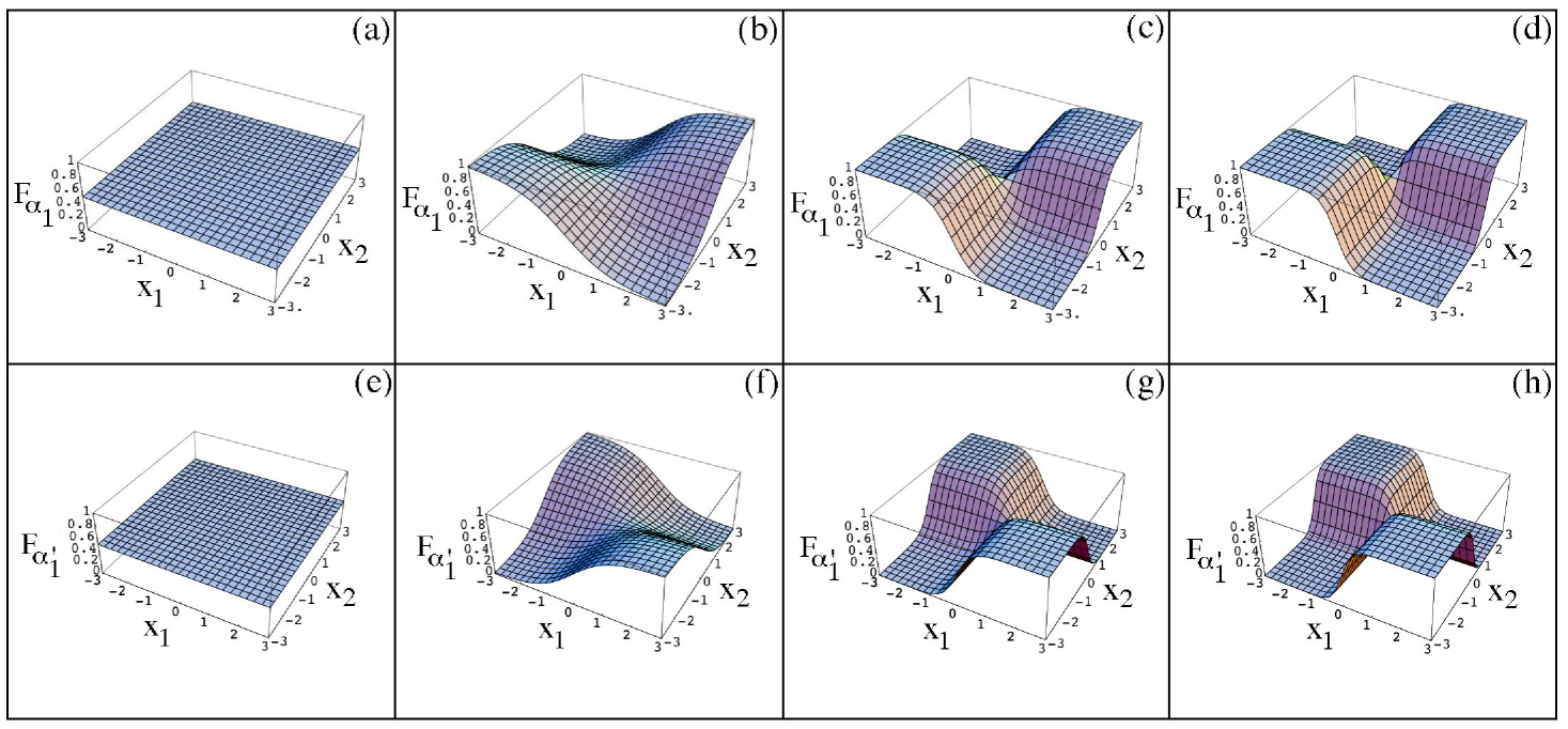
Figure 1: Panels (a), (b), (c) and (d): lower bound for the fidelity with respect to $\left|\alpha\right\rangle_{1}$ $F_{\alpha_{1}}$ as a function of $x_{1}$ and $x_{2}$ at the rescaled atom-cavity interaction times $\varepsilon\tau=$1 (a), $\varepsilon\tau=$5 (b), $\varepsilon\tau=$8 (c) and $\varepsilon\tau=$10 (d). Panels (e), (f), (g) and (h): lower bound for the fidelity with respect to $\left|\alpha^{\prime}\right\rangle_{1}$ $F_{\alpha^{\prime}_{1}}$ as a function of $x_{1}$ and $x_{2}$ at the rescaled atom-cavity interaction times $\varepsilon\tau=$1 (e), $\varepsilon\tau=$5 (f), $\varepsilon\tau=$8 (g) and $\varepsilon\tau=$10 (h). The atomic positions are in units of $\sigma_{x}$ (width of the initial atomic wavepackets). The parameters used are: $\lambda=10^{-5}$m, $\varepsilon=10^{5}$ sec^-1, $m=10^{-26}$ kg and $\sigma_{x}=\lambda/10$ nota-fig1 .

For the sake of simplicity, we consider equal initial translational states for both the atoms with zero mean position and momentum along the $x$-cavity axis. In such a case, the field-deflected wavepackets $\Phi_{0,i}^{+}(x_{i},\tau)$ and $\Phi_{0,i}^{-}(x_{i},\tau)$ ($i=1,2$) have the explicit form Vag-Cus

$$\Phi_{0,i}^{\pm}(x_{i},\tau)=\frac{e^{\mp\frac{ima\tau}{\hbar}x}e^{-\frac{\left(x\pm\frac{a\tau^{2}}{2}\right)^{2}}{4\sigma_{x}^{2}+\frac{i\hbar\tau}{2m}}}}{(2\pi)^{1/4}\sqrt{\sigma_{x}+\frac{i\hbar\tau}{2m\sigma_{x}}}}$$ (29)

where $a=(\hbar k\varepsilon/m)$. Notice that $\Phi_{0,i}^{+}(x_{i},0)=\Phi_{0,i}^{-}(x_{i},0)$. Eq. (29) shows how the wavefunctions $\Phi_{0,i}^{+}(x_{i},\tau)$ and $\Phi_{0,i}^{-}(x_{i},\tau)$ travel with constant acceleration $a$ towards the negative and positive semi-axis, respectively. It follows that, provided the atom-field interaction time is large enough (of the order of some $\varepsilon^{-1}$), the overlap between the two packets becomes negligible and a measurement of the atomic position is able to distinguish them. In Fig. 1 we plot the lower bounds for the fidelity $F_{\alpha_{1}}$ and $F_{\alpha^{\prime}_{1}}$ against $x_{1}$ and $x_{2}$ at the rescaled atom-cavity interaction times $\varepsilon\tau=1,5,8,10$. Notice how at small times both $F_{\alpha_{1}}$ and $F_{\alpha^{\prime}_{1}}$ are non-zero and markedly lower than 1. However, at larger times their maxima start approaching 1 up to the point that, in the considered ranges of $x_{1}$ and $x_{2}$, $F_{\alpha_{1}}=1$ in the domain $x_{1}x_{2}>0$ and $F_{\alpha_{1}}=0$ at $x_{1}x_{2}<0$, whereas $F_{\alpha^{\prime}_{1}}=1$ in the domain $x_{1}x_{2}<0$ and $F_{\alpha_{1}}=0$ at $x_{1}x_{2}>0$. Such regime is reached provided $\varepsilon\tau\simeq 10$ and it is therefore experimentally accessible with present-day cavity coherence times raymond ; nota-regime . In summary, these results provide clear evidence that large enough atom-field interaction times allow to perform efficient teleportation via atomic position measurements.

VI Conclusions

In summary, in this paper we have considered a cavity-QED teleportation scheme that allows to teleport an unknown quantum state between two atoms flying through a cavity via position measurements on their translational degrees of freedom. Among the major advantages of the scheme are the success probability of 1/2 and its ability to be performed both without direct projections onto highly entangled subspaces and with no holonomous constraints on the atom-cavity interaction times to be fulfilled. The detailed measurement process able to give rise to successful teleportation has been explicitly described in order to derive the final reduced density matrix associated with the state of the target qubit. This has allowed us to perform an efficiency analysis of the scheme in terms of two fidelity functions. We have derived a lower bound for each of them as a function of the possible outcomes of the position measurements performed on the two atoms. Our analysis has shown that a few Rabi oscillations are enough in order to attain the maximum efficiency in a wide range of atomic positions.

Together with our previous study TC , these results provide strong evidence that the atomic translational dynamics in cavity QED holds promises as an attractive resource to be harnessed in order to perform quantum information processing tasks. Interestingly, such idea supports a change of perspective given that the atomic translational dynamics has been frequently addressed so far as an unwanted effect that spoils quantum coherent phenomena in cavity-QED systems Vag-Cus ; which-path ; epl-2atoms ; epjd . The use of such degrees of freedom as a tool in order to either improve known quantum information processing schemes, such as the generation of maximally entangled states, or design novel ones is under ongoing investigations.

References

- (1) M. A. Nielsen and I. L. Chuang, Quantum Computation and Quantum Information (Cambridge University Press, Cambridge, U. K., 2000)
- (2) C. H. Bennett, G. Brassard, C. Cr peau, R. Jozsa, A. Peres, and W. K. Wootters, Phys. Rev. Lett. 70, (1993) 1895
- (3) D. Bouwmeester, J.-W. Pan, K. Mattle, M. Eibl, H. Weinfurter, and A. Zeilinger, Nature (London) 390, (1997) 575 ; D. Boschi, S. Branca, F. De Martini, L. Hardy, and S. Popescu, Phys. Rev. Lett. 80, (1998) 1121
- (4) M. A. Nielsen, E. Knill, and R. Laflamme, Nature (London) 396, (1998) 52.
- (5) Q. Zhang, A. Goebel, C. Wagenknecht, Y.-A. Chen (Chen, Yu-Ao), B. Zhao, T. Yang T, A. Mair, J. Schmiedmayer, Nat. Phys. 2, (2006) 678
- (6) J. F. Sherson, H. Krauter, R. K. Olsson, B. Julsgaard, K. Hammerer, I. Cirac, E. S. Polzik, Nature (London) 443, (2006) 557
- (7) J. M. Raimond, M. Brune, and S. Haroche, Rev. Mod. Phys. 73, 565 (2001)
- (8) L. Davidovich, N. Zagury, M. Brune, J. M. Raimond, and S. Haroche, Phys. Rev. A 50, (1994) R895 ; J. I. Cirac, and A. S. Parkins, Phys. Rev. A 50, (1994) R4441 ; S. B. Zheng and G. C. Guo, Phys. Lett. A 232, (1997) 171 ; S. B. Zheng, Opt. Commun. 167, (1999) 111 ; S. Bose, P. L. Knight, M. B. Plenio, and V. Vedral, Phys. Rev. Lett. 83, (1999) 5158 ; S. Bandyopadhyay, Phys. Rev. A 62, (2000) 012308
- (9) L. Vaidman, Phys. Rev. A 49, (1994) 1473
- (10) N.G. de Almeida, R. Napolitano, and M. H. Y. Moussa, Phys. Rev A. 62, (2000) 010101
- (11) S.-B- Zheng, Phys. Rev. A 69, (2004) 064302
- (12) L. Ye, and G.-C. Guo, Phys. Rev. A 70, (2004) 054303; R. W. Chhajlany and A. W jcik, Phys. Rev. A 73, (2006) 016302; L. Ye, and G.-C. Guo, Phys. Rev. A 73, (2004) 016303
- (13) W. B. Cardoso, A. T. Avelar, B. Baseia, and N. G. de Almeida Phys. Rev. A 72, (2005) 045802
- (14) M. Tumminello, and F. Ciccarello, to appear on Phys. Rev. A, arXiv:0706.0173v1 (2007)
- (15) A. Vaglica, Phys. Rev. A 58, (1998) 3856; I. Cusumano, A. Vaglica, and G. Vetri, Phys. Rev. A 66, (2002) 043408
- (16) M. Tumminello, A. Vaglica, and G. Vetri, Europhys. Lett. 65, (2004) 785
- (17) T. Sleator, T. Pfau, V. Balykin, O. Carnal, and J. Mlynek, Phys. Rev. Lett. 68, (1992) 1996; C. Tanguy, S. Reynaud, and C. Cohen-Tannoudji, J. Phys. B 17, (1984) 4623 ; M. Freyberger, and A. M. Herkommer, Phys. Rev. Lett. 72, (1994) 1952 ; A. Vaglica, Phys. Rev. A 54, (1996) 3195
- (18) R. R. Schlicher, Opt. Comm. 70, (1989) 97
- (19) M. Wilkens, Z. Bialynicka-Birula, and P. Meystre, Phys. Rev. A 45, (1992) 477
- (20) For the benefit of the reader, in this paper we restrict to the nodal approximation of the Hamiltonian since the mathematics in the antinodal case is a bit more involved TC ; epjd . Nonetheless, we point out that both the teleportation scheme TC and the efficiency analysis presented in this work hold in the antinodal case as well.
- (21) M. Tumminello, A. Vaglica, and G. Vetri, Europhys. Lett. 66, (2004) 792
- (22) M. Tumminello, A. Vaglica, and G. Vetri, Eur. Phys. J. D 36, (2005) 235
- (23) A. Vaglica, Phys. Rev. A 52, (1995) 2319
- (24) Similarly to the seminal proposal by Bennett et al. bennett , in such cases teleportation is completed after that a 180 degree rotation around the -axis in the internal Hilbert space of atom 1 is performed.
- (25) The considered range for each is such that for the probability to find each atom in the interval is still significant.
- (26) S. Kuhr et al., Appl. Phys. Lett. 90, (2007) 164101
- (27) Actually, this is an overestimated value since a look at Fig. 1 shows how even at shorter strengths of , such as , there is not so a narrow range of position-measurement outcomes that ensure successful teleportation.