Is the quantum adiabatic theorem consistent?

Abstract

The quantum adiabatic theorem states that if a quantum system starts in an eigenstate of the Hamiltonian, and this Hamiltonian varies sufficiently slowly, the system stays in this eigenstate. We investigate experimentally the conditions that must be fulfilled for this theorem to hold. We show that the traditional adiabatic condition as well as some conditions that were recently suggested are either not sufficient or not necessary. Experimental evidence is presented by a simple experiment using nuclear spins.

In classical physics, adiabatic processes do not involve a transfer of heat between system and environment. In quantum mechanics, the adiabatic theorem states that a system that is initially in an eigenstate of the Hamiltonian will remain in this eigenstate if the changes of this Hamiltonian are sufficiently slow Ehrenfest ; Born ; Kato ; Messiah . While this adiabatic theorem (QAT) is a well established fact, it appears to be difficult to formulate a consistent adiabatic condition (QAC), which unambiguously states when the theorem applies and is both necessary and sufficient.

The QAT is critical for the booming of many domains in quantum mechanics. It provides the foundation and insightful interpretation of Landau-Zener transition Landau , the Gell-Mann-Low theorem Gell and Berry’s phase Berry . Quantum adiabatic processes are also used for some quantum algorithms Farhi ; Steffen , which can efficiently solve NP-complete problems. These algorithms are based on the validity of the QAT and a sufficient QAC Roland .

Recently, however, doubts were cast over the consistency of the QAT and the sufficiency of the QAC. Marzlin and Sanders first suggested a possible inconsistency of the QAT Marzlin1 . Although there are some questionable points in their deduction Marzlin2 ; Marzlin3 ; Marzlin4 , their main point resulted in an extended discussion Wu1 . Then Tong et al gave a specific counterexample to show that the traditional QAC is not sufficient for the adiabatic approximation to hold Tong1 . These discussions about QAT and QAC resulted in further investigations such as modification of traditional QAC Tong2 , reexamination of the quantum adiabatic algorithm Wei , and study of QAC in different quantum systems Sarandy . While there is fast progress in the theoretical discussion about QAC and QAT, an unambiguous experimental investigation is certainly important here. However, such experiements still remained a real challenge due to the following reasons: $\left(1\right)$ the conflict between the sufficiently long time during the adiabatic evolution of the time-dependent Hamiltonian in QAT and the severely short coherent time of the real physical system due to the decoherence. $\left(2\right)$ the suitable technique with good quantum controlling during the quantum adiabatic process.

Considering that the coherent time of nuclei spin inside the atom is relatively longer compared to that of other physical systems and nuclear magnetic resonance (NMR) is well developed over the past decades, here we first present a simple and clear-cut experimental investigation of this issue, using a spin-1/2 particle in a rotating magnetic field. We show that, depending on the parameters chosen, the traditional QAC is neither sufficient nor necessary. Then we theoretically compare various newly proposed QAC’s with the traditional one and compare their applicability to our specific system. We also provide further experimental proof to support our theoretical comparison and discuss the character of the different adiabatic conditions.

The quantum adiabatic theorem states that if the energy levels of a time dependent Hamiltonian $H(t)$ are never degenerate and the Hamiltonian varies sufficiently slowly with time, the initial eigenstate of this Hamiltonian will stay close to the instantaneous eigenstate at a later time Messiah .

The widely used qualitative condition that assures the QAT valid is the QAC:

$$|\frac{\langle E_{m}(t)|\dot{E}_{n}(t)\rangle}{E_{m}(t)-E_{n}(t)}|\ll 1,\quad m\neq n,\quad t\in[0,T],$$ (1)

where $E_{m}(t)$ and $|E_{m}(t)\rangle$ are the instantaneous eigenvalues and eigenstates of $H(t)$, and $T$ is the total evolution time. We define the fidelity as the absolute value of the overlap of the actual state and the instantaneous eigenstate: $F(t)=|\langle\Psi(t)|\phi(t)\rangle|$, where $|\Psi(t)\rangle$ is the instantaneous eigenstate of the Hamiltonian and $|\phi(t)\rangle$ is the state that has evolved under the Hamiltonian $H(t)$ from $|\Psi(0)\rangle$. With this definition, the adiabatic theorem can be formulated such that the fidelity F(t) will stay close to 1 if the variation of Hamiltonian meets condition (1).

As a specific Hamiltonian, we choose

$$H(t)=\omega_{0}\frac{\sigma_{z}}{2}+\omega_{1}(\frac{\sigma_{x}}{2}\cos\omega^{\prime}t+\frac{\sigma_{y}}{2}\sin\omega^{\prime}t)$$ (2)

where $\omega_{0}$ is the Larmor frequency, $\omega_{1}$ is the strength of the coupling to a radio frequency(rf) magnetic field, and $\omega^{\prime}$ is the rotation frequency of the rf magnetic field. We investigate the validity of the adiabatic theorem as a function of the strength and frequency of the rf field.

Experiments were performed on ¹³C-labeled CHCl₃ at room temperature using a Bruker AV-400 spectrometer. The experiments were performed on the ¹³C nuclear spin, while the ¹H nuclear spin was decoupled during the whole experiment.

For the sake of convenience, we define two parameters: $R=\omega_{1}/\omega_{0}$ and $K=\omega^{\prime}/\omega_{0}$. In our first experiment, we choose the power of the rf field $\omega_{1}=100Hz$ and $\omega_{0}=1700Hz$, corresponding to $R=0.06\ll 1$.

The initial Hamiltonian $H(0)$ has an eigentstate $|\Psi(0)\rangle=\cos\frac{\theta}{2}|0\rangle+\sin\frac{\theta}{2}|1\rangle$, in which $\theta=\arctan R=\arctan 0.06$. We can prepare this initial state by applying an rf pulse along the y-axis, with a rotation angle $\arctan 0.06$, to the thermal equilibrium state $|0\rangle$.

To realize an evolution determined by the Hamiltonian (2), we use the discrete approach proposed by Steffen Steffen . The rotation of the rf field, at frequency $\omega^{\prime}$, was performed by applying a sequence of small flip-angle pulses, whose phase was initially set to zero and shifted by $\frac{\pi}{36}$ for every pulse.

We consider two specific cases: $K=1$ and $K=10$ in the following. It is easy to prove that in the first case the evolution under the Hamiltonian (2) satisfies the adiabatic condition (1), while in the second case the evolution of the Hamiltonian violates the adiabatic condition seriously.

We first consider the case $K=1$, which means $\omega^{\prime}=\omega_{0}=1700Hz$. Thus the width of each flip-angle pulse can be calculated as $\Delta t=\frac{\left(\pi/36\right)}{2\pi\omega^{\prime}}=8.2\mu s$. We can compute the time that the rf field rotates one circle as $\tau=\frac{2\pi}{\pi/36}\cdot\Delta t=590.4\mu s$. We measure the state of the spin after it evolves $n$ circles, in other word, at the time $t=n\tau$, in which $n$ changes from form $0$ to $15$. We can calculate the fidelities at these time points and the experimental results are summarized as black circles in Fig. 1.

By simply changing the pulse width $\Delta t$ in the above experiment, we can realize the case $K=10$. Here, $\omega^{\prime}=10\omega_{0}=17000Hz$ and $\Delta t=0.82\mu s$. We repeat the same process in the last experiment and the result is presented as red squares in Fig. 1.

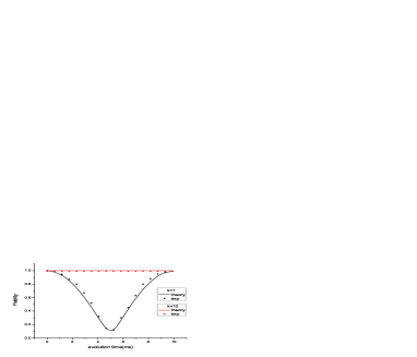
Figure 1: (color online) Measured fidelity when $K=1$ compared to the fidelity when $K=10$. The black curve and red curve are the theoretical results of $K=1$ and $K=10$ respectively. The black circles and red squares are the experimental results of $K=1$ and $K=10$ respectively.

An interesting and exciting phenomenon is that when $K=1$ and the traditional adiabatic condition is satisfied, the state evolves far away from instantaneous eigenstate and the fidelity falls below $0.1$ at $t=5ms$. Therefore, we can conclude that the adiabatic condition is not sufficient. On the other hand, when $K=10$, even though the traditional adiabatic condition is violated, the state is always next to the instantaneous eigenstate and the fidelity remains close to $1$. So the adiabatic condition (1) is not necessary. Synthesizing these two cases, it is evident that the traditional QAC is indeed problematic.

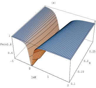
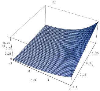
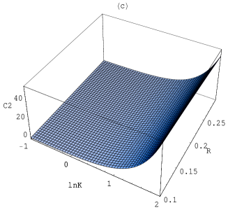
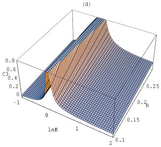
Figure 2: (color online) (a) The minimum fidelity in the process of evolution as a function of $lnK$ and $R$. (b)-(d) show the traditional QAC, Tong’s and Wu’s expression as a function of the same parameters.

Next, we examine the validity of other, more recently proposed adiabatic conditions, again using the Hamiltonian (2). We compare the traditional QAC, Tong’s QAC and Wu’s QAC Tong2 . Analytically solving the Schrödinger equation, we can calculate $F_{min}$, the minimal fidelity of F(t) in the process of evolution:

$$F_{min}=\frac{(1-K)\cos\theta+R\sin\theta}{\sqrt{(1-K)^{2}+R^{2}}}$$ (3)

where $\theta$ was defined earlier. For the sake of convenience, we define $C_{1}$ as the expression in traditional QAC: $C_{1}=|\frac{\langle E_{+}(t)|\dot{E}_{-}(t)\rangle}{E_{+}-E_{-}}|$.

Using fundamental inequalities, Tong et al states that the adiabatic approximation will be reasonable if the Hamiltonian satisfies the following conditions

$$(A) \quad|\frac{\langle E_{m}(t)|\dot{E}_{n}(t)\rangle}{E_{m}-E_{n}}|\ll 1,\quad t\in[0,T],$$ (4)

$$(B) \quad\int_{0}^{T}|(\frac{\langle E_{m}(t)|\dot{E}_{n}(t)\rangle}{E_{m}-E_{n}})^{\prime}|dt\ll 1,$$ (5)

$$(C) \quad\int_{0}^{T}|\frac{\langle E_{m}(t)|\dot{E}_{n}(t)\rangle\langle E_{n}(t)|\dot{E}_{l}(t)\rangle}{E_{m}-E_{n}}|dt\ll 1,$$ (6)

in which $\langle m(t)|\dot{m}(t)\rangle=0$, $m\neq n$, $n\neq l$, and $T$ is the total evolution time. For our system, condition (5) is the strongest of these. Therefore we define $C_{2}=\int_{0}^{T}|(\frac{\langle E_{+}(t)|\dot{E}_{-}(t)\rangle}{E_{+}-E_{-}})^{\prime}|dt$, in which $T$ equals $1/\omega^{\prime}$, a typical evolution time.

On the basis of invariant perturbation theory, Wu et al deduced a modified adiabatic condition

$$|\frac{\langle E_{m}(t)|\dot{E}_{n}(t)\rangle}{E_{m}-E_{n}+\Delta_{nm}}|\ll 1,\quad t\in[0,T].$$ (7)

In the condition (7)

$$\Delta_{nm}=i\langle E_{n}(t)|\dot{E}_{n}(t)\rangle-i\langle E_{m}(t)|\dot{E}_{m}(t)\rangle$$

$$+i\frac{d}{dt}\arg\langle E_{m}(t)|\dot{E}_{n}(t)\rangle$$ (8)

is $U(1)$-invariant under the time-dependent transformation, and it is just the difference of Berry phase between different evolution orbits if it is integrated along a cycle. For the Hamiltonian (2), we can rewrite the condition (7) as $C_{3}=|\frac{\langle E_{+}(t)|\dot{E}_{-}(t)\rangle}{E_{+}-E_{-}+i\langle E_{-}(t)|\dot{E}_{-}(t)\rangle-i\langle E_{+}(t)|\dot{E}_{+}(t)\rangle}|$.

Figure 2 summarizes $F_{min}$, $C_{1}$, $C_{2}$ and $C_{3}$ as functions of $K$ and $R$. In each case, the adiabatic condition $C_{i}\ll 1$ should imply $F_{min}\approx 1$ ($i=1,2,3$). For the traditional QAC (Fig. 2b), we note that at $K\approx 1$, the QAC is fulfilled, but $F_{min}$ falls well below $1$. Conversely, when $K\gg 1$, $F_{min}$ remains close to 1. Apparently, the traditional QAC is neither necessary nor sufficient.

Similarly, adiabatic condition $C_{2}\ll 1$ is fulfilled only for $K\ll 1$. Because $F_{min}\approx 1$ if $K\ll 1$ or $K\gg 1$ (When $R\ll 1$), we can conclude that this adiabatic condition is sufficient but not necessary. The adiabatic condition most suitable to our Hamiltonian is $C_{3}\ll 1$. $C_{3}$ is small where $F_{min}$ is close to 1 and vice versa. For our system, Wu’s adiabatic condition is therefore sufficient as well as necessary.

We have experimentally verified the calculations represented in Fig. 2. In the experiment, we measured the minimum fidelity as a function of $K$ at fixed $R$ and as a function of $R$ at fixed $K$. In this experiment, the average rf field strength was $\omega_{1}=100$ Hz, and we used the same discrete method for the implementation of the time-dependent Hamiltonian as in the first experiment. We changed $K$ from $0.5$ to $1.5$ by varying the width of the flip-angle pulses, and we varied $R$ from $0.05$ to $0.3$ by varying the frequency offset $\omega_{0}$. The most important difference from the first experiment is that here we did not measure the state after a cyclic evolution, at $t=n\tau$, but at the time of the minimum fidelity, $t_{min}=\frac{1}{2\sqrt{(1-K)^{2}\omega_{0}^{2}+\omega_{1}^{2}}}$. As an example, for the parameters $R=0.05$ and $K=0.75$, $t_{min}=980.6\mu s$. The experimental points were not chosen equidistant as a function of $K$, but denser around $K=1$, where the minimum fidelity changes rapidly. The experimental results are represented in Fig. 3; obviously, the agreement with the theoretical predictions of Fig. 2 (represented as the curves in Fig. 3) is more than satisfactory.

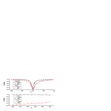
Figure 3: (color online) (a) The fidelity during the evolution measured as a function of $K$. The black circles and red squares are the experimental minimum fidelities for $R=0.05$ and $R=0.1$ respectively. The black and red curves are the theoretical results. (b) The minimum fidelity as a function of $R$. The black circles and red squares represent the experimental data for $K=10$ and $K=1$ respectively. The black and red curves are the theoretical results.

Qualitatively, the observed behavior for the case of $K=1$ can be understood as a resonant phenomenon. Although the perturbation (rf in our experiment) is very small, it can seriously affect the evolution if it contains a frequency component that matches a transition frequency of the system. The traditional QAC and Tong’s condition do not account for resonant effects, but in Wu’s adiabatic condition takes includes it’s effect.

In this experiment, the parameter $R$ reflects the angle between the rotating magnetic field and the z axis. Fig. 3 demonstrates that if the magnetic field is very close to the z axis, the resonance region is narrow. If the angle increases ($R$ increases), the ”resonance” becomes both wider and deeper. If we consider the behavior as a function of $R$, we observe different behaviors, depending on $K$.

Several adiabatic algorithms have been proposed for quantum computing; in most cases, their validity was discussed in terms of the traditional QAC Roland . Since this condition is neither sufficient nor necessary, the validity of these adiabatic algorithms should be re-evaluated. Conversely, if they are designed to fulfill a QAC that is not necessary, these algorithms may not realize their full potential. Although Wu’s QAC seems to be proper in our specific system, it is still not always a sufficient and necessary condition Tong2 . Therefore, finding a QAC that is both sufficient and necessary remains an open question. Finding such a condition will be important for the development of quantum adiabatic algorithms.

In conclusion, we have demonstrated that the traditional adiabatic condition is neither sufficient nor necessary. We found that the most important deviation can be understood as a resonant effect. Rather than concluding that the quantum adiabatic theorem is inconsistent Marzlin1 , we hold that it is important to determine the correct condition for an adiabatic evolution of a quantum system.

- (1) P. Ehrenfest, Ann. Phys 356, 327 (1916).
- (2) M. Born and V. Fock, Z. Phys. 51, 165 (1928).
- (3) T. Kato, J. Phys. Soc. Jpn. 5, 435 (1950).
- (4) A. Messiah, Quantum Mechanics (Dover, New York, 1999).
- (5) L. D. Landau, Phys. Z. Sowjetunion 2, 46 (1932).
- (6) M. Gell-Mann and F. Low, Phys. Rev. 84, 350 (1951).
- (7) M.V. Berry, Proc. R. Soc. London A 392, 45 (1984).
- (8) B. Simon, Phys. Rev. Lett. 51, 2167 (1983).
- (9) Edward Farhi, Jeffrey Goldstone, Sam Gutmann, Joshua Lapan, Andrew Lundgren, Daniel Preda , Science 292, 472 (2001).
- (10) Matthias Steffen, Wim van Dam, Tad Hogg, Greg Breyta, Isaac Chuang,Phys. Rev. Lett. 90, 067903 (2003).
- (11) Jeremie Roland and Nicolas J. Cerf,Phys. Rev. A 65, 042308 (2002).
- (12) Karl-Peter Marzlin, Barry C. Sanders, Phys. Rev. Lett. 93, 160408 (2004).
- (13) Solomon Duki, H. Mathur, Onuttom Narayan, Phys. Rev. Lett. 97, 128901 (2006).
- (14) Jie Ma, Yongping Zhang, Enge Wang, Biao Wu, Phys. Rev. Lett. 97, 128902 (2006).
- (15) Karl-Peter Marzlin, Barry C. Sanders, Phys. Rev. Lett 97, 128903 (2006).
- (16) Zhaoyan Wu and Hui Yang, Phys. Rev. A 72, 012114 (2005).
- (17) D. M. Tong, K. Singh, L. C. Kwek, C. H. Oh, Phys. Rev. Lett. 95, 110407 (2005).
- (18) D. M. Tong, K. Singh, L. C. Kwek, C. H. Oh, Phys. Rev. Lett. 98, 150402 (2007); R. MacKenzie, E. Marcotte, H. Paquette, Phys. Rev. A 73, 042104 (2006); Jian-Lan Chen, Mei-sheng Zhao, Jian-da Wu and Yong-de Zhang, quant-ph/07060299; Jian-da Wu, Mei-sheng Zhao, Jian-lan Chen, Yong-de Zhang, arXiv:0706.0264.
- (19) Zhaohui Wei and Mingsheng Ying, Phys. Rev. A 76, 024304 (2007).
- (20) M. S. Sarandy and D. A. Lidar, Phys. Rev. Lett. 71, 012331 (2005); M. S. Sarandy and D. A. Lidar, Phys. Rev. Lett. 95, 250503 (2005); Han Pu, Peter Maenner, Weiping Zhang, and Hong Y. Ling, Phys. Rev. Lett. 98, 050406 (2007).