Mesoscopic conductance fluctuations in graphene samples

Abstract

Mesoscopic conductance fluctuations in graphene samples at energies not very close to the Dirac point are studied analytically. We demonstrate that the conductance variance $\langle[\delta G]^{2}\rangle$ is very sensitive to the elastic scattering breaking the valley symmetry. In the absence of such scattering (disorder potential smooth at atomic scales, trigonal warping negligible), the variance $\langle[\delta G]^{2}\rangle=4\langle[\delta G]^{2}\rangle_{\text{metal}}$ is four times greater than that in conventional metals, which is due to the two-fold valley degeneracy. In the absence of intervalley scattering, but for strong intravalley scattering and/or strong warping $\langle[\delta G]^{2}\rangle=2\langle[\delta G]^{2}\rangle_{\text{metal}}$. Only in the limit of strong intervalley scattering $\langle[\delta G]^{2}\rangle=\langle[\delta G]^{2}\rangle_{\text{metal}}$. Our theory explains recent numerical results and can be used for comparison with existing experiments.

Introduction. Graphene (a monolayer of graphite) is a novel material Novoselov ; Zhang ; Berger ; Berger2 with the Dirac electronic spectrum. A lot of progress in the theoretical understanding of clean graphene has been made so far (see e.g. Ref. cleangraphene ). For many interesting effects, however, disorder plays a significant role. A peculiar feature of disordered graphene is that its physical properties are sensitive to the scattering processes breaking the valley symmetry.

This sensitivity has been revealed in the behavior of the weak localization (WL) correction to conductivity Khvesh ; WLFalko ; Morpurgo ; AlEf ; WLFalkobilayer . Another famous phenomenon due to disorder that goes along with WL are the mesoscopic conductance fluctuations (CF). CF with variance $\sim e^{2}/\hbar$ are observed in graphene samples experimentally Berger2 ; CFexp1 ; CFexp3 ; CFexp4 , although a detailed analysis has not been reported.

Numerical investigation of CF in graphene has been undertaken recently in Ref. CFnum . The authors have rather unexpectedly found that CF in graphene were considerably stronger than those in conventional metals CFAlt ; CFLeeStone and the variance did not seem to be universal. No clear explanation of this effect was given in Ref. CFnum , although it was argued that the unusual behavior might be due to percolation effects.

Here we develop an analytical theory of conductance fluctuations in diffusive graphene samples at energies not very close to the Dirac point. The results we obtain explain the findings of Ref. CFnum and can be directly used for comparison with the experiments.

Model. We consider a general microscopic model of disorder in graphene. The single-particle Hamiltonian of the system is (we put $\hbar=1$ and recover it later on)

$$\hat{H}_{\bf r}=\hat{H}_{0}+\hat{H}_{\text{w}}+\hat{V}({\bf r}),\mbox{ }\hat{H}_{0}=-iv(1^{KK^{\prime}}\otimes\tau_{\lambda}^{AB})\partial_{\lambda}.$$ (1)

Here $\hat{H}_{\text{w}}=\mu_{\text{w}}\tau_{z}^{KK^{\prime}}\otimes[\tau_{x}(\partial_{x}^{2}-\partial_{y}^{2})-2\tau_{y}\partial_{x}\partial_{y}]^{AB}$ describes weak trigonal warping and $\lambda=x,y$. The Hamiltonian $\hat{H}_{\bf r}$ is a matrix in the tensor product $KK^{\prime}\otimes AB$ of the valley ($KK^{\prime}$) and sub-lattice ($AB$) spaces and $1$, $\tau_{x,y,z}$ are the unity and Pauli matrices. The random disorder potential $\hat{V}({\bf r})$ is Gaussian with the correlation function

$$\langle\hat{V}({\bf r})\otimes\hat{V}({\bf r}^{\prime})\rangle=\{\Lambda_{0}\openone\otimes\openone+\Lambda^{k}_{l}\mathcal{T}_{kl}\otimes\mathcal{T}_{kl}\}\delta({\bf r}-{\bf r}^{\prime}),$$ (2)

where $\openone=1^{KK^{\prime}}\otimes 1^{AB}$, $\mathcal{T}_{kl}=\tau_{k}^{KK^{\prime}}\otimes\tau_{l}^{AB}$, $k,l=x,y,z$. For a given Fermi energy $\epsilon$ the scattering rates (inverse scattering times) are defined as

$$(\gamma_{0},\gamma_{zz},\gamma_{z\perp},\gamma_{\perp z},\gamma_{\perp\perp})\equiv\pi\nu(\Lambda_{0},\Lambda^{z}_{z},\Lambda^{z}_{x,y},\Lambda^{x,y}_{z},\Lambda^{x,y}_{x,y}),$$

where $\nu=\epsilon/(2\pi v^{2})$ is the density of states per one valley and one spin.

In Eq. (2), the term $\propto\gamma_{0}$ arises from remote charge impurities in the substrate, the field of which varies smoothly at atomic scales, while the rest of the terms describe various atomically-sharp defects that break the valley symmetry. Being diagonal in $KK^{\prime}$-space ($\propto~{}\tau_{z}^{KK^{\prime}}$), the terms $\propto\gamma_{zz}$ and $\propto\gamma_{z\perp}$ do not involve the intervalley scattering, but do lift the valley degeneracy by acting differently on the valleys. Such terms describe the intravalley scattering, whereas the terms $\propto\gamma_{\perp z}$ and $\propto\gamma_{\perp\perp}$ are due to

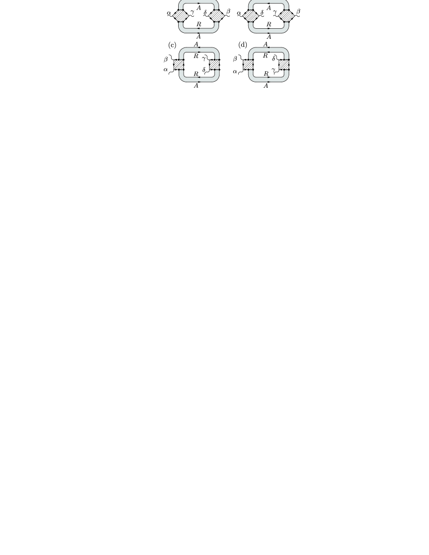
Figure 1: Diagrams for the conductivity correlation function $F_{\alpha\beta,\gamma\delta}(\Delta\epsilon,H,\Delta H)$ [Eq. (10)]. Gray stripes denote diffusons and Cooperons, rendered with lines blocks are Hikami boxes, see Fig. 2. The diagrams (c),(d) with the substitution $\alpha\leftrightarrow\beta$, $\gamma\leftrightarrow\delta$, $R\leftrightarrow A$ must also be considered.

Calculations. We calculate the correlation function

$$F_{\alpha\beta,\gamma\delta}(\Delta\epsilon,H,\Delta H)=\langle\delta\sigma_{\alpha\beta}(\epsilon+\Delta\epsilon,H+\Delta H)\delta\sigma_{\gamma\delta}(\epsilon,H)\rangle$$ (3)

of the conductivities $\sigma_{\alpha\beta}(\epsilon+\Delta\epsilon,H+\Delta H)$ and $\sigma_{\gamma\delta}(\epsilon,H)$ taken at the Fermi energies $\epsilon+\Delta\epsilon$, $\epsilon$ mesoscale and magnetic fields $H+\Delta H$, $H$ ($\alpha,\beta,\gamma,\delta=x,y$ and $\delta\sigma=\sigma-\langle\sigma\rangle$).

We use the averaging technique developed for conventional disordered metals AGD . We assume (i) weak disorder, $\Lambda_{0}/v^{2}\ll 1$, and (ii) diffusive regime, i.e., that the mean free path $l=v/\gamma_{0}$ is much smaller than the size of the sample and the valley-symmetric rate $\gamma_{0}$ is dominant, $\gamma_{0}\gg\gamma_{\{z,\perp\},\{z,\perp\}}$. As it was shown in Ref. AlEf one should first renormalize the velocity $v$ and constants $\Lambda$ [Eq. (2)] solving renormalization group equations and then use them for calculating the localization corrections. This procedure is valid so long as $\epsilon\gtrsim\epsilon_{0}\exp(-\pi v^{2}/\Lambda_{0})$, where $\epsilon_{0}$ is an atomic-scale energy. The same can be done for the correlation function (3) and we further assume that $v$ and $\Lambda$’s have been renormalized. Under these assumptions, the calculations for graphene generalize those for ordinary metals CFAlt ; CFLeeStone and $F_{\alpha\beta,\gamma\delta}(\Delta\epsilon,H,\Delta H)$ is given by the diagrams in Fig. 1.

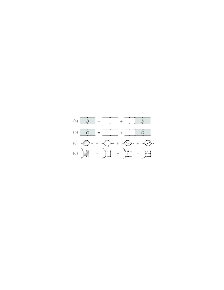
Figure 2: (a),(b) Diagrammatic representation of the integral equations for the diffuson and Cooperon. (c),(d) Hikami boxes. The current vertex renormalized by disorder (dark triangle) equals $\tilde{j}_{\alpha}=2ev(1^{KK^{\prime}}\otimes\tau_{\alpha}^{AB})$.

The arising disorder-averaged products of the exact retarded ($R$) and advanced ($A$) Green’s functions $\hat{\mathcal{G}}^{R,A}$ yield the diffusons and Cooperons defined as:

$$\hat{D}_{\omega}({\bf r},{\bf r}^{\prime})\equiv\langle\hat{\mathcal{G}}^{R}(\varepsilon+\omega,{\bf r},{\bf r}^{\prime})\otimes\hat{\mathcal{G}}^{A}(\varepsilon,{\bf r}^{\prime},{\bf r})\rangle,$$ (4)

$$\hat{C}_{\omega}({\bf r},{\bf r}^{\prime})\equiv\langle\hat{\mathcal{G}}^{R}(\varepsilon+\omega,{\bf r},{\bf r}^{\prime})\otimes\hat{\mathcal{G}}^{A}(\varepsilon,{\bf r},{\bf r}^{\prime})\rangle.$$ (5)

They satisfy the integral equations represented diagrammatically in Fig. 2(a),(b). These equations possess a nontrivial matrix structure acquired from the correlator (2) (dashed lines) and disorder-averaged $\langle\hat{\mathcal{G}}^{R,A}\rangle$ (fermionic lines). Consequently, there exist “high-energy” modes of $\hat{D}$ and $\hat{C}$ with gaps $\sim\gamma_{0}$ as well as “low-energy” modes, which gaps do not contain $\gamma_{0}$ WLFalko ; AlEf . Giving much greater contribution in the diffusive regime, only the latter low-energy modes are of interest here.

The effect of trigonal warping can be taken into account in $\hat{\mathcal{G}}^{R,A}$ up to the second order in $\hat{H}_{\text{w}}$. As a result, the self-energies of the Green’s functions $\langle\hat{\mathcal{G}}^{R,A}\rangle$ acquire the warping rate $\gamma_{\text{w}}=(\mu_{\text{w}}\epsilon/v^{2})^{2}/\gamma_{0}$ and the dashed line in Fig. 2(a),(b), in addition to the correlator (2), also represents the “warping term”

$$\hat{\gamma}_{\text{w}}^{D,C}=\pm\gamma_{\text{w}}(\tau_{z}^{KK^{\prime}}\otimes 1^{AB})_{R}\otimes(\tau_{z}^{KK^{\prime}}\otimes 1^{AB})_{A}$$

with $+$ and $-$ for the diffuson [$D$,(a)] and Cooperon [$C$,(b)], respectively. It appears that, in the low-energy diffuson/Cooperon subspaces, the matrix structure of the warping term $\hat{\gamma}_{\text{w}}^{D,C}$ is identical to that of the intravalley scattering of type $\hat{\gamma}_{zz}=\gamma_{zz}\mathcal{T}_{zz}\otimes\mathcal{T}_{zz}$ in Eq. (2). Therefore, the effect of warping on the low-energy diffusion modes of $\hat{D}$ and $\hat{C}$ is not any different from that of the intravalley scattering $\propto\gamma_{zz}$ and the effect of warping could be taken into account by the substitution $\gamma_{zz}\rightarrow\gamma_{zz}+\gamma_{\text{w}}$.

Resolving the matrix-structure of the equations in Fig. 2(a),(b), we obtain:

$$\hat{D}_{\omega}({\bf r},{\bf r}^{\prime})=\frac{\pi\nu}{16}\left\{\left[D^{0}_{\omega}+D^{1}_{\omega}+2D^{2,3}_{\omega}\right]1\otimes 1+\left[D^{0}_{\omega}+D^{1}_{\omega}-2D^{2,3}_{\omega}\right]\tau_{z}\otimes\tau_{z}+[D^{0}_{\omega}-D^{1}_{\omega}]\tau_{\lambda}\otimes\tau_{\lambda}\right\}\otimes(1\otimes 1+\tau_{k}\otimes\tau_{k})$$ (6)

$$\hat{C}_{\omega}({\bf r},{\bf r}^{\prime})=\frac{\pi\nu}{16}\left\{\left[2C^{2,3}_{\omega}+C^{1}_{\omega}+C^{0}_{\omega}\right]1\otimes 1+\left[2C^{2,3}_{\omega}-C^{1}_{\omega}-C^{0}_{\omega}\right]\tau_{z}\otimes\tau_{z}+[C^{1}_{\omega}-C^{0}_{\omega}]\tau_{\lambda}\otimes\tau_{\lambda}\right\}\otimes(1\otimes 1-\tau_{k}\otimes\tau_{k})$$ (7)

In Eqs. (6) and (7), the tensor products are ordered as $(R\otimes A)_{KK^{\prime}}\otimes(R\otimes A)_{AB}$, $\lambda=x,y$, and $k=x,y,z$. The diffuson/Cooperon components $D^{i}_{\omega}=D^{i}_{\omega}({\bf r},{\bf r}^{\prime})$ and $C^{i}_{\omega}=C^{i}_{\omega}({\bf r},{\bf r}^{\prime})$, $i=0,1,2,3$, satisfy the equations

$$\{-i\omega-D\nabla_{D,C}^{2}+\Gamma_{i}+\gamma_{\text{inel}}\}(D,C)^{i}_{\omega}({\bf r},{\bf r}^{\prime})=\delta({\bf r}-{\bf r}^{\prime}),$$ (8)

where $\nabla_{D}=\nabla-i(e/c)\Delta{\bf A}({\bf r})$, $\nabla_{C}=\nabla-i(e/c)[2{\bf A}({\bf r})+\Delta{\bf A}({\bf r})]$, the vector potentials ${\bf A}({\bf r})$, $\Delta{\bf A}({\bf r})$ correspond to $H$ and $\Delta H$, respectively, $D=v^{2}/\gamma_{0}$ is the diffusion coefficient, and $\gamma_{\text{inel}}$ is the inelastic scattering rate due to, e.g., electron-electron or electron-phonon interactions. The elastic scattering rates $\Gamma_{i}$ due to disorder equal

$$\Gamma_{0}=0,\mbox{ }\Gamma_{1}=4\gamma_{\perp},\mbox{ }\Gamma_{2}=\Gamma_{3}=2\gamma_{\perp}+2\gamma_{z}+2\gamma_{\text{w}},$$ (9)

where the total intervalley $\gamma_{\perp}=\gamma_{\perp z}+2\gamma_{\perp\perp}$ and intravalley $\gamma_{z}=\gamma_{zz}+2\gamma_{z\perp}$ scattering rates were introduced.

The Cooperon in the form of Eq. (7) has been obtained earlier WLFalko ; AlEf , whereas the form (6) of the diffuson is obtained here for the first time. Note that for a given $i$ the rates $\Gamma_{i}$ [Eq. (9)] entering the corresponding diffuson $D_{\omega}^{i}$ and Cooperon $C_{\omega}^{i}$ modes are identical. The fact that the insensitive to various phase-breaking phenomena diffuson $\hat{D}$ does contain the rates $\gamma_{z}$, $\gamma_{\perp}$, and $\gamma_{\text{w}}$ nn means that the effects of the intravalley and intervalley scattering and of the trigonal warping should never be understood as a suppression of electron interference alone.

Results. Calculating the diagrams in Fig. 1, for the correlation function of conductivities [Eq. (3)] we obtain

$$F_{\alpha\beta,\gamma\delta}(\Delta\epsilon,H,\Delta H)=\langle\delta\sigma_{\alpha\beta}(\epsilon+\Delta\epsilon,H+\Delta H)\delta\sigma_{\gamma\delta}(\epsilon,H)\rangle=(2_{s}\,2_{v}e^{2}D)^{2}\int\frac{d\varepsilon d\varepsilon^{\prime}}{(2\pi)^{2}}\frac{dn(\varepsilon)}{d\varepsilon}\frac{dn(\varepsilon^{\prime})}{d\varepsilon^{\prime}}\frac{1}{\mathcal{S}^{2}}$$

$$\times\int d{\bf r}\,d{\bf r}^{\prime}\,\sum_{i=0}^{3}\left\{\delta_{\alpha\gamma}\delta_{\beta\delta}|D^{i}_{\omega}({\bf r},{\bf r}^{\prime})|^{2}+\delta_{\alpha\delta}\delta_{\beta\gamma}|C^{i}_{\omega}({\bf r},{\bf r}^{\prime})|^{2}+\frac{1}{2}\delta_{\alpha\beta}\delta_{\gamma\delta}\text{Re}[D^{i}_{\omega}({\bf r},{\bf r}^{\prime})D^{i}_{\omega}({\bf r}^{\prime},{\bf r})+C^{i}_{\omega}({\bf r},{\bf r}^{\prime})C^{i}_{\omega}({\bf r}^{\prime},{\bf r})]\right\},$$ (10)

where $\omega=\varepsilon-\varepsilon^{\prime}+\Delta\epsilon$, $\mathcal{S}$ is the sample area, $n(\varepsilon)=1/[\exp(\varepsilon/T)+1]$ is the Fermi distribution function, and the factors $2_{s}$ and $2_{v}$ originate from the dimensionality of the spin and valley spaces (the indices $s$ and $v$ emphasize their origin).

Equation (10), together with Eqs. (6)-(9), constitutes the main result of our work. The key feature characterizing graphene is that different diffuson and Cooperon modes $i$ enter Eq. (10). The magnitude of mesoscopic fluctuations is thus determined by the strength of elastic scattering processes breaking the valley symmetry. When all such effects are negligible, the result (10) for graphene is $(2_{v})^{2}=4$ times greater than that for conventional metals CFAlt ; CFLeeStone due to the two-fold valley degeneracy. Note that at $H=\Delta H=0$ one has $D_{\omega}^{i}=C_{\omega}^{i}$ and for a given $i$ the diffuson and Cooperon contribute equally.

To be specific, below we consider the case of a rectangular sample with length $\mathcal{L}_{x}$ and width $\mathcal{L}_{y}$, occupying the area $0<x<\mathcal{L}_{x}$, $0<y<\mathcal{L}_{y}$, and attached to ideal leads at $x=0$ and $x=\mathcal{L}_{x}$. The conductance $G=G_{xx}$ in the $x$ direction is related to the conductivity $\sigma_{xx}$ as $G=\sigma_{xx}\mathcal{L}_{y}/\mathcal{L}_{x}$. From Eq. (10), at $T,\gamma_{\text{inel}}\ll\epsilon^{*}_{x}$, where $\epsilon_{x}^{*}=\pi^{2}D/\mathcal{L}_{x}^{2}$ is the Thouless energy for the $x$ dimension, for the conductance correlation function $\mathcal{F}(\Delta\epsilon)=\langle\delta G(\epsilon+\Delta\epsilon)\delta G(\epsilon)\rangle=(\mathcal{L}_{y}/\mathcal{L}_{x})^{2}F_{xx,xx}(\Delta\epsilon,H,0)$ we obtain

$$\mathcal{F}(\Delta\epsilon) = \alpha_{H}\left[\frac{2_{s}\,2_{v}e^{2}D}{2\pi}\right]^{2}\frac{1}{\mathcal{L}_{x}^{4}}$$ (11)

$$\times \sum_{i=0}^{3}\sum_{\bf q}\left\{2|D^{i}_{\Delta\epsilon}({\bf q})|^{2}+\text{Re}[D^{i}_{\Delta\epsilon}({\bf q})]^{2}\right\},$$

where $D_{\Delta\epsilon}^{i}({\bf q})=1/(-i\Delta\epsilon+D{\bf q}^{2}+\Gamma_{i})$ are the spatial eigenmodes of the diffuson, ${\bf q}^{2}=q_{x}^{2}+q_{y}^{2}$, $q_{x}=\pi n_{x}/\mathcal{L}_{x}$, $n_{x}=1,2,\ldots,$ and $q_{y}=\pi n_{y}/\mathcal{L}_{y}$, $n_{y}=0,1,\ldots.$ In Eq. (11), the factor $\alpha_{H}$ accounts for the sensitivity of the Cooperons to the magnetic field in the two limiting cases: $\alpha_{H}=1$ for $H\ll H^{*}$ and $\alpha_{H}=1/2$ for $H\gg H^{*}$, where $H^{*}=(c/e)/\mathcal{L}_{x}^{2}$. The conductance variance $\mathcal{F}(\Delta\epsilon=0)=\langle[\delta G]^{2}\rangle$ following from Eq. (11) equals

$$\langle[\delta G]^{2}\rangle=3\alpha_{H}\left[\frac{2_{s}\,2_{v}e^{2}}{2\pi\hbar}\right]^{2}\sum_{i=0}^{3}\mathcal{R}(\mathcal{L}_{i},\mathcal{L}_{x},\mathcal{L}_{y}),$$ (12)

$$\mathcal{R}(\mathcal{L}_{i},\mathcal{L}_{x},\mathcal{L}_{y})=\frac{1}{\pi^{4}\mathcal{L}_{x}^{4}}\sum_{n_{x}=1}^{\infty}\sum_{n_{y}=0}^{\infty}\left[\frac{1}{\mathcal{L}_{i}^{2}}+\frac{n_{x}^{2}}{\mathcal{L}_{x}^{2}}+\frac{n_{y}^{2}}{\mathcal{L}_{y}^{2}}\right]^{-2},$$ (13)

where $\mathcal{L}_{i}^{2}=\pi^{2}D/\Gamma_{i}$. For both narrow ($\mathcal{L}_{y}\ll\mathcal{L}_{x}$) and wide ($\mathcal{L}_{y}\gg\mathcal{L}_{x}$) samples, the contribution of a given mode $i$ to Eq. (13) is unsuppressed if $\mathcal{L}_{i}\gg\mathcal{L}_{x}$ and equals:

$$\mathcal{R}_{0}=\mathcal{R}(\infty,\mathcal{L}_{x},\mathcal{L}_{y})=\left\{\begin{array}[]{ll}1/90,&\mathcal{L}_{y}\ll\mathcal{L}_{x},\\ \zeta(3)\mathcal{L}_{y}/(4\pi^{3}\mathcal{L}_{x}),&\mathcal{L}_{x}\ll\mathcal{L}_{y}.\end{array}\right.$$

Wide samples are thus more attractive for the observation of unsuppressed CF. In this case the length $\mathcal{L}_{i}$ has to be greater than only the shorter dimension $\mathcal{L}_{x}$ (equivalently, $\Gamma_{i}\ll\epsilon^{*}_{x}$), but can be arbitrary compared to $\mathcal{L}_{y}$.

The limiting cases of Eq. (12) for different strengths of the scattering processes can be summarized as follows:

$$\langle[\delta G]^{2}\rangle=\frac{2_{v}^{2}}{4}\alpha_{\gamma}\langle[\delta G]^{2}\rangle_{\text{m}},\mbox{ }\langle[\delta G]^{2}\rangle_{\text{m}}=12\alpha_{H}\left[\frac{2_{s}e^{2}}{2\pi\hbar}\right]^{2}\mathcal{R}_{0},$$ (14)

where the conductance variance $\langle[\delta G]^{2}\rangle_{\text{m}}$ for a conventional metal CFAlt ; CFLeeStone was introduced. The coefficient $\alpha_{\gamma}$ gives the number of diffusion modes $i$ that contribute (i.e., for which $\Gamma_{i}\ll\epsilon_{x}^{*}$) to CF, see Table 1. As follows from Eq. (9), the mode $i=0$ (“pseudo-spin singlet”) is unaffected by any of the scattering mechanisms, the mode $i=1$ (“triplet, 0”) can be suppressed by the intervalley scattering only, and the modes $i=2,3$ (“triplet, $\pm 1$”) can be suppressed by both intervalley and intravalley scattering and by trigonal warping. Note that trigonal warping does affect CF, in the same way as intravalley scattering does.

(i) When all the effects are negligible, $\gamma_{\perp},\gamma_{z},\gamma_{\text{w}}\ll\epsilon^{*}_{x}$, all four modes contribute equally, $\alpha_{\gamma}=4$, and $\langle[\delta G]^{2}\rangle=4\langle[\delta G]^{2}\rangle_{\text{m}}$ is four times greater than that for a conventional metal. This is explained by an additional two-fold valley degeneracy described by the factor $2_{v}$ in Eq. (14).

(ii) If the intervalley scattering is weak, $\gamma_{\perp}\ll\epsilon^{*}_{x}$, but either the intravalley scattering or the trigonal warping are sufficiently strong, $\gamma_{z}\gg\epsilon^{*}_{x}$ or $\gamma_{\text{w}}\gg\epsilon^{*}_{x}$, then the two modes $i=0,1$ contribute, while the modes $i=2,3$ are suppressed. In this case $\alpha_{\gamma}=2$ and $\langle[\delta G]^{2}\rangle=2\langle[\delta G]^{2}\rangle_{\text{m}}$ is two times greater than that for a metal.

(iii) Finally, if the intervalley scattering is strong, $\gamma_{\perp}\ll\epsilon^{*}_{x}$, and the intravalley scattering $\gamma_{z}$ and trigonal warping $\gamma_{\text{w}}$ rates are arbitrary compared to $\epsilon^{*}_{x}$, then all triplet modes $i=1,2,3$ are suppressed, and only the gapless mode $i=0$ contributes. In this case $\alpha_{\gamma}=1$ and $\langle[\delta G]^{2}\rangle=\langle[\delta G]^{2}\rangle_{\text{m}}$ coincides with that for a metal.

	$\gamma_{z}\ll\epsilon^{*}_{x}$ and $\gamma_{\text{w}}\ll\epsilon^{*}_{x}$	$\gamma_{z}\gg\epsilon^{*}_{x}$ or $\gamma_{\text{w}}\gg\epsilon^{*}_{x}$
$\gamma_{\perp}\ll\epsilon^{*}_{x}$	4	2
$\gamma_{\perp}\gg\epsilon^{*}_{x}$	1	1

Table 1: The number $\alpha_{\gamma}$ of the diffusion modes contributing to the conductance variance in graphene for different intervalley $\gamma_{\perp}$, intravalley $\gamma_{z}$ and trigonal warping $\gamma_{\text{w}}$ scattering rates. The value of $\alpha_{\gamma}$ also gives the ratio of the conductance variance in graphene to that in conventional metal, $\langle[\delta G]^{2}\rangle_{\text{graphene}}=\alpha_{\gamma}\langle[\delta G]^{2}\rangle_{\text{metal}}$, see Eq. (14).

The conductances fluctuations in graphene were studied numerically in Ref. CFnum (see Fig. 3 therein). For atomically-sharp disorder, a plateau $\langle[\delta G]^{2}\rangle_{\text{plateau}}\approx\langle[\delta G]^{2}\rangle_{\text{m}}$ in the dependence of $\langle[\delta G]^{2}\rangle$ on the disorder strength $\Lambda_{0}/v^{2}$ was obtained, which clearly corresponds to the case (iii). For atomically-smooth disorder, a wide peak in the dependence of $\langle[\delta G]^{2}\rangle$ on $\Lambda_{0}/v^{2}$ with maximum $\langle[\delta G]^{2}\rangle_{\text{max}}\approx(4.5-5)\langle[\delta G]^{2}\rangle_{\text{m}}$ at $\Lambda_{0}/v^{2}\sim 1$ was obtained. We believe this situation corresponds to the case (i), the maximum value being close to our prediction. We emphasize that our theory, just like that of Refs. CFAlt ; CFLeeStone , requires both weak disorder ($\Lambda_{0}/v^{2}\ll 1$) and the diffusive regime [$l=v/\gamma_{0}\ll\mathcal{L}=\min(\mathcal{L}_{x},\mathcal{L}_{y})$]. The reason for having a peak, rather than a plateau, for smooth disorder in Ref. CFnum is that the range of $\Lambda_{0}/v^{2}$, where both these conditions are met, is quite narrow. The diffusive regime is not reached until disorder becomes strong ($\Lambda_{0}/v^{2}\gtrsim 1$), while for smaller values of $\Lambda_{0}/v^{2}\ll 1$ the system is simply in the ballistic regime $l\gtrsim\mathcal{L}$. This is supported by direct check of parameters ($l/\mathcal{L}\sim 0.1$ for $\Lambda_{0}/v^{2}\sim 1$ and thus $l/\mathcal{L}\sim 1$ for $\Lambda_{0}/v^{2}\sim 0.1$ ) and by an improving tendency (earlier upsurge of $\langle[\delta G]^{2}\rangle$ with increasing $\Lambda_{0}/v^{2}\ll 1$) for larger samples (filled vs. open symbols).

Our theory thus helps understand the findings of Ref. CFnum without assuming the existence of percolation paths and nonergodicity as was done by the authors. The ergodicity implies equivalence of averaging over disorder and the Fermi energy (or magnetic field), $\langle f[G(\epsilon)]\rangle\doteq\lim_{\Delta\epsilon\rightarrow\infty}\frac{1}{\Delta\epsilon}\int_{\epsilon-\Delta\epsilon/2}^{\epsilon+\Delta\epsilon/2}d\epsilon^{\prime}f[G(\epsilon^{\prime})].$ For $f[G(\epsilon)]=G(\epsilon)$, this is clearly true, if $\mathcal{F}(\Delta\epsilon)\rightarrow 0$ as $\Delta\epsilon\rightarrow\infty$, see Eq. (11). This asymptotic of $\mathcal{F}(\Delta\epsilon)$ is determined by the behavior of the diffusion modes $D^{i}_{\Delta\epsilon}({\bf q})$ at large energies $\Delta\epsilon$ and, in this respect, graphene is not any different from an ordinary metal CFAKL . One can estimate $\mathcal{F}(\Delta\epsilon)\propto\int^{+\infty}_{\sqrt{\Delta\epsilon/D}}q\,dq\,\frac{1}{q^{4}}\propto\frac{D}{\Delta\epsilon}$ for $\Delta\epsilon\gg\epsilon_{x}^{*},\epsilon_{y}^{*}$. The proof for $f[G(\epsilon)]=[G(\epsilon)]^{m}$, $m>1$, is analogous. Thus, the ergodic hypothesis for graphene holds. The violation of ergodicity in Ref. CFnum occured near the Anderson metal-insulator transition, and might be due to the fact that averaging over energy was mixing extended and localized states.

Conclusion. We have developed a theory of conductance fluctuations in monolayer graphene samples. We expect our findings presented in the Results section to be also completely applicable to bilayer graphene samples.

We thank SFB Transregio 12 for financial support.

References

• (1) K.S. Novoselov et al., Nature 438, 197 (2005); K. Novoselov et al., Nature Physics 2, 177 (2006).
• (2) Y. Zhang et al., Phys. Rev. Lett. 94,176803 (2005); Y. Zhang et al., Nature 438, 201 (2005).
• (3) C. Berger et al., J. Phys. Chem. B 108 19912 (2004); J.S. Bunch et al., Nano Lett. 5, 287 (2005).
• (4) C. Berger et al., Science 312, 1191 (2006).
• (5) V.P. Gusynin and S.G. Sharapov, Phys. Rev. Lett. 95, 146801 (2005); D. A. Abanin, P.A. Lee, and L.S. Levitov, Phys. Rev. Lett. 96, 176803 (2006); J. Tworzydlo et al., Phys. Rev. Lett. 96, 246802 (2006); V.V. Cheianov and V.I. Falko, Phys. Rev. B 74, 041403 (2006); M.I. Katsnelson, Europhys. J. B 51, 157 (2006), Europhys. J. B 52, 151 (2006); I. L. Aleiner, D. E. Kharzeev, and A. M. Tsvelik, Phys. Rev. B 76, 195415 (2007); V.V. Cheianov, V.I. Fal’ko, B.L. Altshuler, Science 315, 1252 (2007).
• (6) D. V. Khveshchenko, Phys. Rev. Lett. 97, 036802 (2006).
• (7) E. McCann et al., Phys. Rev. Lett. 97, 146805 (2006).
• (8) A. F. Morpurgo and F. Guinea, Phys. Rev. Lett. 97, 196804 (2006).
• (9) I. L. Aleiner and K. B. Efetov, Phys. Rev. Lett. 97, 236801 (2006).
• (10) K. Kechedzhi et al., Phys. Rev. Lett. 98, 176806 (2007).
• (11) S. V. Morozov et. al., Phys. Rev. Lett. 97, 016801 (2006).
• (12) H. B. Heersche et al., Nature 446, 56 (2007).
• (13) R. V. Gorbachev et al., Phys. Rev. Lett. 98, 176805 (2007); arXiv:0708.1700; F. V. Tikhonenko et al., arXiv:0707.0140.
• (14) A. Rycerz, J. Tworzydlo, and C.W.J. Beenakker, Europhys. Lett. 79, 57003 (2007).
• (15) B.L. Altshuler, JETP Lett. 41, 648 (1985); B. L. Altshuler and D. E. Khmelnitskii, JETP Lett. 42, 359 (1985); B. L. Altshuler and B. I. Shklovskii, Sov. Phys. JETP 64, 127 (1986).
• (16) A.D. Stone, Phys. Rev. Lett. 54, 2692 (1985); P.A. Lee and A.D. Stone, Phys. Rev. Lett. 55, 1622 (1985).
• (17) We are interested in the dependence on $\Delta\epsilon$ at mesoscopic scales set by the Thouless energy of the sample and therefore neglect $\Delta\epsilon$ compared to $\epsilon$ in quantities like the density of states $\nu$, etc.
• (18) A.A. Abrikosov, L.P. Gorkov, and I.E. Dzyaloshinskii, Methods of Quantum Field Theory in Statistical Physics, Prentice Hall, New York (1963).
• (19) However, the density-density correlation function $P_{\omega}({\bf r},{\bf r}^{\prime})=2_{s}\,2_{v}\nu[\delta({\bf r}-{\bf r}^{\prime})+i\omega D_{\omega}^{0}({\bf r},{\bf r}^{\prime})]$, obtained from Eq. (6), is expressed solely through the gapless mode $D_{\omega}^{0}$, as one would expect from the particle conservation law.
• (20) B.L. Altshuler, V.E. Kravtsov, and I.V. Lerner, JETP Lett. 43, 441 (1986).