Curvature Interaction in Collective Space

Abstract

For the Riemannian space, built from the collective coordinates used within nuclear models, an additional interaction with the metric is investigated, using the collective equivalent to Einstein’s curvature scalar. The coupling strength is determined using a fit with the AME2003 ground state masses. An extended finite-range droplet model including curvature is introduced, which generates significant improvements for light nuclei and nuclei in the trans-fermium region.

PACS numbers:21.60Ev;02.40.Ky;21.10.Dr; 21.10.Gv; 04.62.+v

1 Introduction

The use of collective models for a description of collective aspects of nuclear motion has proven considerably successful during the past decades. Calculating life-times of heavy nuclei [1], [2], [3], fission yields [4], giving insight into phenomena like cluster-radioactivity [5], [6], bimodal fission or modeling the ground state properties of triaxial nuclei [7] - remarkable results have been achieved by introducing an appropriate set of collective coordinates, like length, deformation, neck or mass-asymmetry [8] for a given nuclear shape and investigating its dynamic properties.

We start with the classical Hamiltonian function

$$H=T+V_{0}$$ (1)

introducing a collective potential $V_{0}$, depending on $N$ collective coordinates $\{q^{i},i=1,...,N\}$,

$$V_{0}(q^{i})=E_{\textrm{macro}}(q^{i})+E_{\textrm{mic}}(q^{i})$$ (2)

with a macroscopic contribution $E_{\textrm{macro}}$ based on e.g. the liquid drop model and a microscopic contribution $E_{\textrm{mic}}$, which mainly contains the shell and pairing energy, and the classical kinetic energy $T$

$$T=\frac{1}{2}B_{ij}\,\dot{q}^{i}\dot{q}^{j}$$ (3)

with collective mass parameters $B_{ij}$.

There are several common methods to generate the collective mass parameters $B_{ij}$, e.g. the cranking model [10] or irrotational flow models are used.

We want to emphasize the fact, that via the relation

$$B_{ij}=m_{A}\,g_{ij}=m_{u}A\,g_{ij}$$ (4)

($m_{A}$ is the mass of the nucleus, $m_{u}=931.5$ MeV is the mass unit and $A$ is the number of nucleons) the collective masses may be interpreted geometrically, defining the metric tensor $g_{ij}$, which fully determines the geometric properties of the collective Riemannian space.

Quantization of the classical Hamiltonian[9] results in the collective Schrödinger equation

$$\hat{S}_{0}\Psi(q^{i},t)=\Big{(}-\frac{\hbar^{2}}{2\,m_{A}}\frac{1}{\sqrt{g}}\partial_{i}g^{ij}\sqrt{g}\partial_{j}-i\hbar\partial_{t}+V_{0}\Big{)}\Psi(q^{i},t)=0$$ (5)

which is the central starting point for a discussion of nuclear collective phenomena.

An alternative approach starts with the Lagrangian density ${\cal L}_{0}$

$${\cal L}_{0}=\frac{\hbar^{2}}{2\,m_{A}}g^{ij}(\partial_{i}\Psi^{*})(\partial_{j}\Psi)+\frac{i\hbar}{2}(\Psi^{*}\frac{\partial\Psi}{\partial t}-\frac{\partial\Psi^{*}}{\partial t}\Psi)-\Psi^{*}V_{0}\Psi$$ (6)

Variation with respect to $\Psi^{*}$ and $\Psi$ yields the above Schrödinger equation.

From this point of view it is remarkable, that obvious extensions of this Lagrangian density have been discussed in other branches of physics, e.g. cosmology or string theory, but have been neglected within the framework of nuclear collective models until now.

Therefore in the following we will introduce a curvature interaction in collective space and discuss the consequences for the prediction of nuclear binding energies.

2 Curvature in collective space

In order to investigate the influence of non vanishing curvature in collective space, we consider an additional interaction with the collective metric, which is determined by the collective mass parameters.

We extend the Lagrangian density

$${\cal L}={\cal L}_{0}-\frac{\hbar^{2}}{2\,m_{A}}\xi\Psi^{*}R\Psi$$ (7)

introducing the Einstein curvature scalar $R$ as an invariant measure for collective curvature. The coupling strength is parametrized with $\xi$.

Variation of this Lagrangian density results in an additional potential term

$$V=V_{0}+\frac{\hbar^{2}}{2m_{A}}\xi R$$ (8)

Since the collective mass parameters are known, $R$ can be calculated. As a starting point the Riemann curvature tensor is given by

$${R^{\alpha}}_{\eta\beta\gamma}=\partial_{\gamma}\Gamma^{\alpha}_{\beta\eta}-\partial_{\beta}\Gamma^{\alpha}_{\eta\gamma}+\Gamma^{\alpha}_{\tau\gamma}\Gamma^{\tau}_{\beta\eta}-\Gamma^{\alpha}_{\tau\beta}\Gamma^{\tau}_{\gamma\eta}$$ (9)

with the Christoffel symbols of second kind [11]

$$\Gamma^{\mu}_{\kappa\sigma}=\frac{1}{2}g^{\nu\mu}(\partial_{\kappa}g_{\nu\sigma}+\partial_{\sigma}g_{\nu\kappa}-\partial_{\nu}g_{\kappa\sigma})$$ (10)

The Riemann curvature tensor may be contracted to get the Ricci tensor

$$R_{\eta\gamma}={R^{\alpha}}_{\eta\alpha\gamma}$$ (11)

and finally we obtain the Einstein curvature scalar $R$ via:

$$R={R^{\eta}}_{\eta}$$ (12)

The explicit form of this curvature term depends on the specific choice of collective coordinates.

In order to examine the consequences and physical interpretation of this additional new term we choose the symmetric two-center shell model including elliptical deformations [12], which can be solved fully analytically. This model is widely used in the description of symmetric fusion reactions and contains the Nilsson model as a limiting case, which will turn out to be a useful property for a physical interpretation.

3 Exact solution for the symmetric two-center shell model

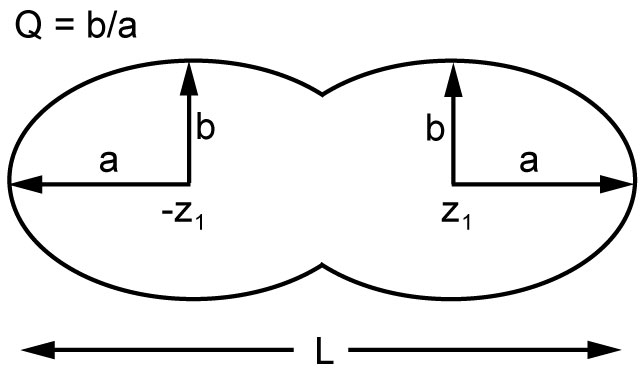
Figure 1: geometry of the symmetric two-center shell model

As an illustrative, exactly solvable scenario we consider the nuclear shape given by two intersecting rotationally symmetric ellipsoids. Introducing two collective coordinates $q^{i}$ namely, the ellipsoidal deformation $Q=b/a$ and the total elongation $L$ the shape $P(z,q^{i})$ is given by (see figure 1):

$$P(z,q^{i})=Q\sqrt{a^{2}-(z\mp z_{1})^{2}}$$ (13)

where the geometric quantities semi axis $a$ and center position of ellipsoids $z_{1}$ are determined by the definition of $L$ and by the requirement of volume conservation, which yields in the case of connected fragments with $R_{0}=r_{0}A^{1/3}$:

$$L = 2(a+z_{1})$$ (14)

volume $$= (4/3)\pi{R_{0}}^{3}=2\,(2/3)\,\pi Q^{2}(a^{3}+\frac{3}{2}a^{2}z_{1}-\frac{1}{2}z_{1}^{3})$$ (15)

These equations may be simplified introducing the dimensionless quantities

$$\alpha = Q^{2/3}\,a/R_{0}$$ (16)

$$\gamma_{1} = Q^{2/3}\,z_{1}/R_{0}$$ (17)

$$\lambda = Q^{2/3}\,L/(2R_{0})$$ (18)

Equations (16)-(18) define a transformation to a new set of coordinates $(\lambda,Q)$.
We obtain:

$$\alpha = \frac{2+\lambda^{3}}{3\,\lambda^{2}}$$ (19)

$$\gamma_{1} = \frac{2\,({\lambda}^{3}-1)}{3\,{\lambda}^{2}}$$ (20)

which is independent of $Q$. Thus, the shape geometry is fully determined for a given set of collective coordinates $(\lambda,Q)$.

$1\leq\lambda\leq 4^{1/3}$ describes connected fragments, where $\lambda=1$ is the compound nucleus and $\lambda=4^{1/3}$ is the scission point and $\lambda>4^{1/3}$ describes separated fragments. $Q<1$ describes prolate and $Q>1$ oblate shapes.

We now apply the Werner-Wheeler-formalism[13] to calculate the collective masses $B_{ij}$, which are directly correlated to the metric tensor $g_{ij}$ according to (4). We choose this method, since masses are determined by shape geometry only and the procedure itself is well defined. Using the abbreviation

$$\Theta=\ln(\frac{4-{\lambda}^{3}}{4+2\,{\lambda}^{3}})$$ (21)

the components of the metric tensor $g_{ij}$ result as

$$g_{\lambda\lambda} = \frac{{R_{0}}^{2}{(2+{\lambda}^{3})}^{2}}{324\,Q^{4/3}\,{\lambda}^{12}}{\times}$$

$$\Big{(}3\,(Q^{2}-16)\,{\lambda}^{9}+4\,(Q^{2}-4)\,[24\,{\lambda}^{3}-3\,{\lambda}^{6}+{({\lambda}^{3}-4)}^{2}\,(2+{\lambda}^{3})\,\Theta]\Big{)}$$

$$g_{\lambda Q} = -\frac{{R_{0}}^{2}}{108\,Q^{7/3}\,{\lambda}^{2}}(2+\lambda^{3})\,\Big{(}6\,\lambda^{3}+Q^{2}\,(4-{\lambda}^{3})\Big{)}$$ (23)

$$g_{QQ} = \frac{{R_{0}}^{2}}{810\,Q^{10/3}\,\lambda}\Big{(}12\,{\lambda}^{3}\,(5+{\lambda}^{3})+Q^{2}\,(40-5\,{\lambda}^{3}+{\lambda}^{6})\Big{)}$$ (24)

A coordinate transformation from the coordinate set $(\lambda,Q)$ to the original $(L,Q)$ using

$$g_{ij}=\frac{\partial x^{m}}{\partial x^{i}}\frac{\partial x^{n}}{\partial x^{j}}g_{mn}$$ (25)

yields the final result for connected shapes in the range $1\leq\lambda\leq 4^{1/3}$

$$g_{LL} = \frac{{(2+{\lambda}^{3})}^{2}}{1296{\lambda}^{12}}\,\times$$

$$\Big{(}3(Q^{2}-16)\lambda^{9}+4(Q^{2}-4)[8\lambda^{3}(3-\lambda^{3})+(4-\lambda^{3})^{2}(2+\lambda^{3})\Theta]\Big{)}$$

$$g_{LQ} = \frac{R_{0}\,(2+{\lambda}^{3})}{1944\,Q^{5/3}{\lambda}^{11}}\,\times$$

$$\Big{(}3{\lambda}^{3}[(Q^{2}+14){\lambda}^{9}+8(Q^{2}-4)(16+6\,{\lambda}^{3}-3{\lambda}^{6})]+$$

$$8(Q^{2}-4)(-8-2{\lambda}^{3}+{\lambda}^{6})^{2}\Theta\Big{)}$$

$$g_{QQ} = \frac{{R_{0}}^{2}}{7290\,Q^{10/3}{\lambda}^{10}}\,\times$$

$$\Big{(}(48+69\,Q^{2}){\lambda}^{15}+(Q^{2}-4)[15{\lambda}^{3}(256+224{\lambda}^{3}-31{\lambda}^{9})+$$

$$40{({\lambda}^{3}-4)}^{2}{(2+{\lambda}^{3})}^{3}\Theta]\Big{)}\quad\quad\quad\quad\quad\quad\quad\quad\quad\quad 1\leq\lambda\leq 4^{1/3}$$

A similar calculation for separated fragments with $\lambda\geq 4^{1/3}$ yields

$$g_{LL} = \frac{1}{4}$$ (29)

$$g_{LQ} = \frac{R_{0}/3}{2^{1/3}\,Q^{5/3}}$$ (30)

$$g_{QQ} = \frac{2^{1/3}\,(12+Q^{2}){R_{0}}^{2}}{45\,Q^{10/3}}\quad\quad\quad\quad\quad\quad\quad\quad\quad\quad\quad\lambda>4^{1/3}$$ (31)

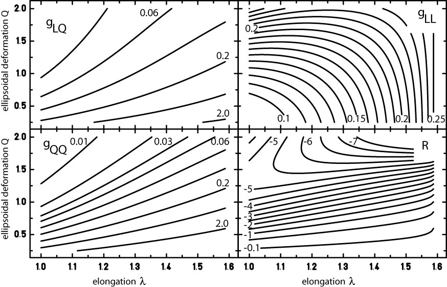
Figure 2: metric tensor components $g_{LQ}$ (upper left), $g_{LL}$ (upper right), $g_{QQ}$ (lower left) and curvature scalar $R$ (lower right) for the symmetric two center shell model, normalized setting $R_{0}=1$

Given the metric tensor $g_{ij}$, the curvature scalar $R(L,Q)$ can easily be calculated.

Figure 2 shows the elements of the metric tensor $g_{ij}$ and the resulting curvature scalar $R$. For connected fragments with $\lambda\leq 4^{1/3}$ a non vanishing curvature scalar $R(L,Q)$ exists. This is a direct consequence of the volume conservation condition (see (15)).

For prolate and moderately oblate shapes ($Q\leq 1.7$) with a fixed Q, the curvature scalar starts with a negative value, which tends to $0$ with increasing $\lambda$ up to the scission point. For oblate shapes ($Q\geq 1.7$) with a fixed Q, $R$ decreases with increasing $\lambda$ down to the scission point.

For separated fragments we obtain $R=0$. This discontinuity of the curvature scalar at the scission point is a direct consequence of the underlying simple geometry, the derivative of the shape is not defined at the contact point of the two ellipsoids. This can be avoided by smoothing the shape appropriately, resulting in a smooth curvature term at the scission point, the resulting model has to be solved numerically though.

The curvature minimizing shape is not a sphere, but a slightly deformed, oblate shape, due to the fact, that the subject of our considerations is not the curvature of a given shape, but curvature of the collective space, generated by the Werner-Wheeler-masses.
In case of a single deformed ellipsoid ($\lambda=1$) $R$ is explicitly given as:

$$R(Q)=\frac{-720\,Q^{16/3}\,(-25+36\,\ln(2))\,(-67+96\,\ln(2))}{R_{0}^{2}\,(2+Q^{2})^{2}\,[-2+(Q^{2}-4)\,(-67+96\,\ln(2))]^{2}}$$ (32)

and finally, for a sphere ($Q=1$) this reduces to $R_{\textrm{sphere}}$:

$$R_{\textrm{sphere}}=-4.3599\frac{1}{R_{0}^{2}}$$ (33)

Since $R$ is an invariant under coordinate transformations, the shape may be described by any appropriate set of coordinates, which obey the transformation rule given in (25). Consequently, for the symmetric two center shell model, which we discussed here as an example, the coordinate sets $(L,Q)$,$(\lambda,Q)$, $(\lambda,\beta=1/Q)$ or $(\Delta z,\beta)$ where $\Delta z$ is the two-center distance, are equivalent. They lead to different mass parameters, but yield the same $R$. In that sense, the curvature scalar is a unique, outstanding property of a given shape geometry.

4 Determination of the coupling constant

In order to get an estimate for the curvature coupling constant, we will now investigate the influence of an additional curvature term by a fit of experimentally known ground state masses of nuclei.

For reasons of simplicity, we assume the ground state of nuclei being of ellipsoidal form only, neglecting higher order multipoles. Therefore the shapes are described by $(\lambda=1,Q)$, depending on only one collective coordinate $Q$.

We define the relative curvature energy $B_{R}$ with respect to the spherical compound nucleus $(\lambda=1,Q=1)$ as

$$B_{R} = R(\lambda=1,Q)/R_{\textrm{sphere}}$$ (34)

$$= 9\,Q^{16/3}\Big{(}\frac{199-288\ln(2)}{(2+Q^{2})[266-67Q^{2}+96(Q^{2}-4)\ln(2)]}\Big{)}^{2}$$ (35)

An additional curvature potential term $V_{R}$ is defined

$$V_{R}(a_{R},Q) = +\frac{\hbar^{2}}{2m_{A}}\xi R_{\textrm{sphere}}B_{R}$$ (36)

$$= -a_{R}B_{R}A^{-5/3}$$ (37)

where we introduced the curvature-energy constant $a_{R}$, which will be determined now.

Table 1: determination of volume-energy $a_{v}$, volume-asymmetry $k_{v}$, surface-energy $a_{s}$, surface-asymmetry $k_{s}$ and curvature energy $a_{R}$ constants within the original FRLDM, FRLDM2003 fitted with AME2003 experimental masses and FRLDMC, which corresponds to FRLDM plus curvature term and resulting root-mean-square deviations $\Delta_{\textrm{rms}}$ from AME2003 experimental data

constants	FRLDM	FRLDM2003	FRLDMC
$a_{v}$	16.00126 MeV	16.00496 MeV	16.01890 MeV
$k_{v}$	1.92240 MeV	1.93167 MeV	1.92882 MeV
$a_{s}$	21.18466 MeV	21.18770 MeV	21.25974 MeV
$k_{s}$	2.345 MeV	2.35968 MeV	2.34955 MeV
$a_{R}$	-	-	529.95850 MeV
$\Delta_{\textrm{rms}}$	0.821 MeV	0.815 MeV	0.764 MeV

Our choice for an appropriate macroscopic model is the finite range liquid drop model FRLDM. It is widely used and documented in detail [14].

We shall vary only a subset of parameters, namely, the volume-energy $a_{v}$, the volume-asymmetry $k_{v}$, the surface-energy $a_{s}$ and the surface-asymmetry $k_{s}$ constants, which generate the major contributions for the calculated masses, keeping all other parameters at their original values.

We define the finite range liquid drop model with curvature (FRLDMC):

$$\textrm{FRLDMC}(a_{v},k_{v},a_{s},k_{s},a_{R},Q) =\textrm{FRLDM}(a_{v},k_{v},a_{s},k_{s},Q)+V_{R}(a_{R},Q)$$ (38)

Theoretical masses $m_{\textrm{th}}$ are then obtained, including the microscopic corrections $E_{\textrm{mic}}$

$$m_{\textrm{th}} =\textrm{FRLDMC}+E_{\textrm{mic}}$$ (39)

and are compared with the AME2003 experimental masses [15]. For conversion from quadrupole moments $\beta_{2}$ to ellipsoidal deformations $Q$ we use the relation:

$$Q=1-\frac{3}{2}\sqrt{\frac{5}{4\pi}}\beta_{2}$$ (40)

As a measure for the quality of the fit, we tabulate the root mean square deviation

$$\Delta_{\textrm{rms}}=\sqrt{\frac{1}{N}\sum^{N}(m_{\textrm{exp}}-m_{\textrm{th}})^{2}}$$ (41)

Results are collected in table 1. The first column lists the original FRLDM parameter set, followed by results for FRLDM2003, which corresponds to an actualized FRLDM-parameter set for AME2003 masses and finally results for FRLDMC, which corresponds to the original FRLDM including the curvature term are presented.

The corresponding $\Delta_{\textrm{rms}}$-values indicate a significant improvement of the new, extended FRLDMC-model. Especially for light nuclei and in the region of trans lead elements improvements are significant, as shown in table 3, where errors for different $Z$-regions are listed.

For light nuclei this is due to the $A^{-5/3}$ behavior of the curvature energy, since this term contributes most to the total binding energy for light nuclei, e.g. for ${}^{16}\textrm{O}=5.21$ MeV, while for heavy nuclei, this term becomes negligible e.g. for ${}^{208}\textrm{Pb}=0.07$ MeV. The improvement indicates, that the additional Riemann curvature term is a useful extension for a collective model.

Since overestimating masses for heavy nuclei is a known shortcoming of FRLDM, Nix et al.[14] introduced the finite range droplet model (FRDM), whose major improvement is an additional empirical exponential term of the form

$$-CA\exp^{-\gamma A^{1/3}}\bar{\epsilon}$$ (42)

Using original parameters, this term simulates an A-dependence, which is close to the collective curvature term, derived in this work.

Table 2: determination of volume-energy $a_{v}$, surface-energy $a_{s}$, charge-asymmetry $c_{a}$ and curvature energy $a_{R}$ constants within the original FRDM, FRDM2003 fitted with AME2003 experimental masses and FRDMC, which corresponds to FRDM plus curvature term and resulting root-mean-square deviations $\Delta_{\textrm{rms}}$ from AME2003 experimental data

constants	FRDM	FRDM2003	FRDMC
$a_{v}$	16.247 MeV	16.2401 MeV	16.2467 MeV
$a_{s}$	22.92 MeV	22.8812 MeV	22.9159 MeV
$c_{a}$	0.436 MeV	0.4368 MeV	0.4332 MeV
$a_{R}$	-	-	172.676 MeV
$\Delta_{\textrm{rms}}$	0.679 MeV	0.674 MeV	0.655 MeV

Therefore we expect a reduced influence of an additional curvature term within the framework of FRDM.
To proof this hypothesis, we define the finite range drop model with curvature (FRDMC) and vary with respect to the subset of most important parameters, $a_{v}$ volume-energy, $a_{s}$ surface-energy and $c_{a}$ charge-asymmetry constants, keeping all other parameters fixed at their original values.

$$\textrm{FRDMC}(a_{v},a_{s},c_{a},a_{R},Q)=\textrm{FRDM}(a_{v},a_{s},c_{a},Q)+V_{R}(a_{R},Q)$$ (43)

Once again theoretical masses $m_{\textrm{th}}$ and experimental masses were fitted. Results are listed in table 2.

As expected, the curvature-energy constant $a_{R}$ is reduced by a factor 3, which results in an absolute contribution to the total binding energy of about $1.7$ MeV for ¹⁶O.

For light and trans fermium nuclei we achieve a significant improvement with the extended FRDMC, compared to the original FRDM. The additional curvature term makes the FRDMC the best model available for the description of ground state masses in the full range of the nuclear table.

Thus, within both extended models, the FRLDMC and the FRDMC, the existence of a curvature term is supported. The coupling strength $\xi$, derived from fits, setting $r_{0}=1.16$ fm results as $\xi=7.8$ for FRLDMC and $\xi=2.5$ for FRDMC respectively.

Table 3: root-mean-square deviations $\Delta_{\textrm{rms}}$ from AME2003 experimental data in MeV for different $Z$-Regions

Z/model	8-20	20-40	40-60	60-80	80-100	$\geq$ 100
FRLDM	1.716	0.857	0.568	0.654	0.746	1.091
FRLDMC	1.307	0.900	0.582	0.814	0.494	0.508
FRDM	1.447	0.871	0.579	0.449	0.388	0.512
FRDMC	1.287	0.887	0.547	0.448	0.407	0.487

5 Conclusion

Based on a purely geometric interpretation of collective mass-parameters, the collective curvature scalar term has been introduced. For the geometry of the symmetric two-center shell model this term has been derived analytically. Interpreting this term as an additional potential term with the explicit form $V\sim A^{-5/3}$, we have investigated the influence of this term within the framework of two new macroscopic models: The finite range liquid drop model with curvature (FRLDMC) and the finite range droplet model with curvature (FRDMC).

Significant improvements have been found especially for light nuclei and for trans-fermium elements. Thus, the new models allow a more precise description of nuclear ground state properties.

Therefore the collective curvature scalar as a manifestation of interaction with curved collective space plays a substantial role in nuclear physics e.g. for strong asymmetric fission, cluster-radioactivity or prediction of super-heavy element properties as well as other branches of physics like cosmology or star-formation.

References

- [1] W. D. Myers and W. J. Swiatecki Nucl. Phys. 81 (1966) 1
- [2] J. Grumann, U. Mosel, B. Fink and W. Greiner Z. Phys. 228 (1969) 371
- [3] A. Staszczak, A. Baran and W. Nazarewicz (2012) arXiv:1208.1215 [nucl-th]
- [4] H. J. Lustig, J. A. Maruhn and W. Greiner J. Phys. G 6 (1980) L25
- [5] A. Sandulescu, D. N. Poenaru and W. Greiner Soviet Journal of Particles and Nuclei 11 (1980) 528
- [6] D. N. Poenaru and W. Greiner Phys. Scr. 44 (1991) 427
- [7] P. Möller, R. Bengtsson, B. G. Carlsson, P. Olivius, T. Ichikawa, H. Sagawa and A. Iwamoto At. Nucl. Data Tables 94(5) (2008) 758
- [8] J. A. Maruhn and W. Greiner Z. Phys. 251 (1972) 431
- [9] D. Podolsky and W. Pauli Phys. Rev. 32 (1928) 812
- [10] D. Inglis Phys. Rev 56 (1950) 1059
- [11] R. Adler, M. Bazin and M. Schiffer, Introduction to General Relativity, (McGraw-Hill New York 1965)
- [12] D. Scharnweber and W. Greiner Nucl. Phys. A 164 (1971) 257
- [13] I. Kelson Phys. Rev. B 136 (1964) 1667
- [14] P. Möller, J. R. Nix, W. D. Myers and W. J. Swiatecki At. Nucl. Data Tables 59 (1995) 185
- [15] G. Audi, O. Bersillon, J. Blachot and A. H. Wapstra Nucl. Phys. A 729 (2003) 3