Design of experiments and biochemical network inference

Abstract.

Design of experiments is a branch of statistics that aims to identify efficient procedures for planning experiments in order to optimize knowledge discovery. Network inference is a subfield of systems biology devoted to the identification of biochemical networks from experimental data. Common to both areas of research is their focus on the maximization of information gathered from experimentation. The goal of this paper is to establish a connection between these two areas coming from the common use of polynomial models and techniques from computational algebra.

1. Introduction

Originally introduced in PRW , the field of algebraic statistics focuses on the application of techniques from computational algebra and algebraic geometry to problems in statistics. One initial focus of the field was the design of experiments, beginning with PW ; Ri . An early exposition of a basic mathematical relationship between problems in the design of experiments and computational commutative algebra appeared in Ro . The basic strategy of Ro and other works is to construct an algebraic model, in the form of a polynomial function with rational coefficients, of a fractional factorial design. The variables of the polynomial function correspond to the factors of the design. One can then use algorithmic techniques from computational commutative algebra to answer a variety of questions, for instance about the classification of all polynomial models that are identified by a fractional design.

If $\mathbf{p}_{1},\ldots,\mathbf{p}_{r}$ are the points of a fractional design with $n$ levels, then the key algebraic object to be considered is the ideal of points $I$ that contains all polynomials with rational coefficients that vanish on all $\mathbf{p}_{i}$. (See the appendix for a review of basic concepts from commutative algebra.) The form of the polynomials in different generating sets of this ideal is of special interest. In particular, we are interested in so-called interpolator polynomials which have a unique representation, given an explicit choice of generating set. An interpolator polynomial $f(x_{1},\ldots,x_{n})$ has the property that if $b_{1},\ldots,b_{r}$ is a response to the design given by the $\mathbf{p}_{i}$, then $f(\mathbf{p}_{i})=b_{i}$.

Strikingly similar constructions have been used recently to solve an entirely different set of problems related to the inference of intracellular biochemical networks, such as gene regulatory networks, from experimental observations. Relatively recent technological breakthroughs in molecular biology have made possible the simultaneous measurement of many different biochemical species in cell extracts. For instance, using DNA microarrays one can measure the concentration of mRNA molecules, which provide information about the activity levels of the corresponding genes at the time the cell extract was prepared. Such network-level measurements provide the opportunity to construct large-scale models of molecular systems, including gene regulatory networks.

Here, an experimental observation consists of the measurement of $n$ different quantities at $r$ successive time points, resulting in a time course of $n$-dimensional real-valued vectors $\mathbf{p}_{1},\ldots,\mathbf{p}_{r}$. The number $r$ of experimental observations is typically very small compared to the number $n$ of quantities measured, due in part to the considerable expense of making measurements. In recent years there has been tremendous research activity devoted to the development of mathematical and statistical tools to infer the entire network structure from such a limited set of experimental measurements.

Inferring networks from data is a central problem in computational systems biology, and several approaches have been developed using a variety of approaches. Models range from statistical models such as Bayesian networks to dynamic models such as Markov chains and systems of differential equations. Another modeling framework is that of finite dynamical systems such as Boolean networks. A method proposed in LS uses such data to construct a multi-state discrete dynamical system

$$f=(f_{1},\ldots,f_{n}):k^{n}\longrightarrow k^{n}$$

over a finite field $k$ such that the coordinate functions $f_{i}$ are polynomials in variables $x_{1},\ldots,x_{n}$ corresponding to the $n$ biochemical compounds measured. The system $f$ has to fit the given time course data set, that is, $f(\mathbf{p}_{i})=\mathbf{p}_{i+1}$ for $i=1,\ldots,r-1$. The goal is to infer a “best” or most likely model $f$ from a given data set which specifies a fraction of the possible state transitions of $f$. An advantage to working in a finite field is that all functions $k^{n}\rightarrow k$ are represented by polynomials. An important, and unanswered, question is to design biological experiments in an optimal way in order to infer a likely model with high probability. One complicating factor is that biochemical networks tend to be highly nonlinear.

In this paper, we describe the two approaches and point out the similarities between the two classes of problems, the techniques used to solve them, and the types of questions asked.

2. Design of experiments

In this section we provide a description of the computational algebra approach to experimental design given in Ro ; PRW . Let $\mathcal{D}$ be the full factorial design with $n$ factors. We make the additional simplifying assumptions that each factor has the same number $p$ of levels, resulting in $p^{n}$ points for $\mathcal{D}$. A model for the design is a function

$$f:\mathcal{D}\longrightarrow\mathbb{Q},$$

that is, $f$ maps each point of $\mathcal{D}$ to a measurement. Instead of using the field $\mathbb{Q}$ for measurements, one may choose other fields such as $\mathbb{C}$ or a finite field. From here on we will denote the field by $k$. It is well-known that any function from a finite number of points in $k^{n}$ to $k$ can be represented by a polynomial, so we may assume that $f$ is a polynomial in variables $x_{1},\ldots,x_{n}$ with coefficients in $k$.

Definition 2.1.

A subset $\mathcal{F}=\{\mathbf{p}_{1},\ldots,\mathbf{p}_{r}\}\subset\mathcal{D}$ is called a fraction of $\mathcal{D}$.

We list three important problems in the design of experiments:

1. Identify a model for the full design $\mathcal{D}$ from a suitably chosen fraction $\mathcal{F}$.

2. Given information about features of the model, such as a list of the monomials (power products) appearing in it, design a fraction $\mathcal{F}$ which identifies a model for $\mathcal{D}$ with these features.

3. Given a fraction $\mathcal{F}$, which models can be identified by it?

These problems can be formulated in the language of computational algebra making them amenable to solution by techniques from this field. The fraction $\mathcal{F}$ is encoded by an algebraic object $I(\mathcal{F})$, an ideal in the polynomial ring $k[x_{1},\ldots,x_{n}]$. This ideal contains all those polynomial functions $g\in k[x_{1},\ldots,x_{n}]$ such that $g(\mathbf{p}_{i})=0$ for all $i=1,\ldots,r$. It is called the ideal of points of the $\mathbf{p}_{i}$ and contains all polynomials confounded by the points in $\mathcal{F}$. Here we assume that the points are distinct. We will see that one can draw conclusions about $\mathcal{F}$ from its ideal of confounding polynomials. In particular, since any two polynomial models on $\mathcal{F}$ that differ by a confounding polynomial are identical on $\mathcal{F}$, it is advantageous to choose models from the quotient ring $R=k[x_{1},\ldots,x_{n}]/I(\mathcal{F})$ rather than from the polynomial ring itself.

It can be shown that the ring $R$ is isomorphic to the vector space $k^{s}$, and we need to study possible vector space bases for $R$ consisting of monomials. This can be done using Gröbner bases of the ideal $I(\mathcal{F})$ (see the appendix). For each choice of a term order for $k[x_{1},\ldots,x_{n}]$, that is, a special type of total ordering of all monomials, we obtain a canonical generating set $G=\{g_{1},\ldots,g_{s}\}$ for $I(\mathcal{F})$. We obtain a canonical $k$-basis for the vector space $R\cong k^{s}$ by choosing all monomials which are not divisible by the leading monomial of any of the $g_{i}$. We can then view each polynomial in $R$ as a $k$-linear combination of the monomials in the basis.

To be precise, let $\{T_{1},\ldots,T_{t}\}$ be the set of all monomials in the variables $x_{1},\ldots,x_{n}$ which are not divisible by the leading monomial of any $g_{i}$. Then each element $f\in R$ can be expressed uniquely as a $k$-linear combination

$$f=\sum_{j=1}^{t}a_{j}T_{j},$$

with $a_{j}\in k$. Suppose now that we are given a fractional design $\mathcal{F}=\{\mathbf{p}_{1},\ldots,\mathbf{p}_{r}\}$ and an experimental treatment resulting in values $f(\mathbf{p}_{i})=b_{i}$ for $i=1,\ldots,r$. If we now evaluate the generic polynomial $f$ at the points $\mathbf{p}_{i}$, we obtain a system of linear equations

$$a_{1}T_{1}(\mathbf{p}_{1})+\ldots+a_{t}T_{t}(\mathbf{p}_{1}) = b_{1},$$

$$\vdots$$

$$a_{1}T_{1}(\mathbf{p}_{r})+\ldots+a_{t}T_{t}(\mathbf{p}_{r}) = b_{r}.$$

We can view these equations as a system of linear equations in the variables $a_{j}$ with the coefficients $T_{j}(\mathbf{p}_{i})$. We now obtain the main criterion for the unique identifiability of a model $f$ from the fraction $\mathcal{F}$.

Theorem 2.2.

[Ro, , Thm. 4.12] Let $\mathcal{X}=\{\mathbf{p}_{1},\ldots,\mathbf{p}_{r}\}$ be a set of distinct points in $k^{n}$, and let $f$ be a linear model with monomial support $\mathcal{S}=\{T_{1},\ldots,T_{t}\}$, that is, $f=\sum_{i}a_{i}T_{i}$. Let $X(\mathcal{S},\mathcal{X})$ be the $(r\times t)$-matrix whose $(i,j)$-entry is $T_{j}(\mathbf{p}_{i})$. Then the model $f$ is uniquely identifiable by $\mathcal{X}$ if and only if $X(\mathcal{S},\mathcal{X})$ has full rank.

In this section we have given a brief outline of a mathematical framework within which one can use tools from computational algebra to address the three experimental design problems listed above. In the next section we will describe a similar set of problems and a similar approach to their solution in the context of biochemical network modeling.

3. Biochemical network inference

Molecular biology has seen tremendous advances in recent years due to technological breakthroughs that allow the generation of unprecedented amounts and types of data. For instance, it is now possible to simultaneously measure the activity level of all genes in a cell extract using DNA microarrays. This capability makes it possible to construct large-scale mathematical models of gene regulatory and other types of cellular networks, and the construction of such models is one of the central foci of computational systems biology. The availability of obtaining experimental measurements for large numbers of entities that are presumed to be interconnected in a network drives the need for the development of network inference algorithms. We will focus on the mathematical aspects of this problem for the rest of the section. More biological background can be found in LS .

We consider a dynamic network with $n$ variables $x_{1},\ldots,x_{n}$. These could represent products of $n$ genes in a cell extract from a particular organism, say yeast. It is known that cellular metabolism and other functions are regulated by the interaction of genes that activate or suppress other genes and form a complex network. Suppose we are given a collection of pairs of simultaneous measurements of these variables:

$$(\mathbf{p}_{1},\mathbf{q}_{1}),\ldots,(\mathbf{p}_{r},\mathbf{q}_{r}),$$

with $\mathbf{p}_{i},\mathbf{q}_{i}$ points in $\mathbf{R}^{n}$. For gene networks, each of these measurements could be obtained from a DNA microarray. Each pair $(\mathbf{p}_{i},\mathbf{q}_{i})$ is to be interpreted as follows. The variables in the network are initialized at $\mathbf{p}_{i}$ and subsequently the network transitions to $\mathbf{q}_{i}$. This might be done through a perturbation such as an experimental treatment, and $\mathbf{p}_{i}$ represents the network state immediately after the perturbation and $\mathbf{q}_{i}$ represents the network state after the network has responded to the perturbation. Sometimes the measurement pairs are consecutive points in a measured time course. In this case the pairs above consist of consecutive time points. Typically the number $n$ of variables is orders of magnitude larger than the number $r$ of measurements, in contrast to engineering applications where the reverse is true (OR where $r$ is on the order of $n$). For instance the network may contain hundreds or thousands of genes, from which only 10 or 20 experimental measurements are collected.

Example 3.1.

Consider the following time course for a biochemical network of 3 genes, labeled $x_{1},x_{2},$ and $x_{3}$.

$x_{1}$	$x_{2}$	$x_{3}$
1.91	3.30	1.98
1.50	1.42	1.99
1.42	1.31	0.03
0.83	1.96	1.01
0.97	2.08	1.01

Each gene’s expression levels were measured at 5 consecutive time points and each entry represents a measurement. While the data are given in tabular form, we could have also represented the data as the pairs of network states

$$\left((1.91,3.30,1.98),(1.50,1.42,1.99)\right)$$

$$\left((1.50,1.42,1.99),(1.42,1.31,0.03)\right)$$

$$\left((1.42,1.31,0.03),(0.83,1.96,1.01)\right)$$

$$\left((0.83,1.96,1.01),(0.97,2.08,1.01)\right).$$

Network inference problem. Given input-output measurements $\{(\mathbf{p}_{i},\mathbf{q}_{i})\}$, infer a model of the network that produced the data.

One can consider a variety of different model types. First it is of interest to infer the directed graph of causal connections in the network, possibly with signed edges indicating qualitative features of the interactions. Dynamic model types include systems of differential equations, Boolean networks, Bayesian networks, or statistical models, to name a few. In light of the fact that DNA microarray data contain significant amounts of noise and many necessary parameters for models are unknown at this time, it suggests itself to consider a finite number of possible states of the variables $x_{i}$ rather than treating them as real-valued. This is done by Bayesian network inference methods, for instance. The issue of data discretization is a very subtle one. On the one hand, discrete data conform more to actual data usage by experimentalists who tend to interpret, e.g., DNA microarray data in terms of genes fold changes of regulation compared to control. On the other hand, a lot of information is lost in the process of discretizing data and the end result typically depends strongly on the method used. In the extreme case, one obtains only two states corresponding to a binary ON/OFF view of gene regulation. In our case, a strong advantage of using discrete data is that it allows us to compute algorithmically the whole space of admissible models for a given data set, as described below. Nonetheless, the result typically depends on the discretization method and much work remains to be done in understanding the effect of different discretization methods. Once the variables take on values in a finite set $k$ of states, it is natural to consider discrete dynamical systems

$$F:k^{n}\longrightarrow k^{n}.$$

As mentioned, the dynamics is generated by repeated iteration of the mapping $F$. In order to have mathematical tools available for model construction and analysis, one can make the assumption that $k$ is actually a finite field rather than simply a set. In practice this is easily accomplished, since the only ingredient required is the choice of a finite state set that has cardinality a power of a prime number. With these additional assumptions our models are polynomial dynamical systems

$$F=(f_{1},\ldots,f_{n}):k^{n}\longrightarrow k^{n},$$

with $f_{\ell}\in k[x_{1},\ldots,x_{n}]$ for $\ell=1,\ldots,n$. (As remarked above, any function from a finite set of points into a field can be represented as a polynomial function.) The $\ell$-th polynomial function $f_{\ell}$ describes the transition rule for gene $x_{\ell}$ and hence $f_{\ell}$ is called the transition function for $x_{\ell}$.

Returning to the network inference problem, we can now rephrase it in the following form: Given the state transitions $\{(\mathbf{p}_{i},\mathbf{q}_{i})\}$, find a polynomial dynamical system (or polynomial model) $F$ such that $F(\mathbf{p}_{i})=\mathbf{q}_{i}$.

This problem can be solved one node at a time, that is, one transition function at a time. This “local” approach to inference then begins with a collection $\{\mathbf{p}_{i}\}$ of points, and we are looking for transition functions $f_{\ell}\in k[x_{1},\ldots,x_{n}]$ that satisfy the condition that $f_{\ell}(\mathbf{p}_{i})=b_{i}$, where $b_{i}$ is the $\ell$-th entry in $\mathbf{q}_{i}$.

Example 3.2.

Let

$$(\mathbf{p}_{1},\mathbf{q}_{1}) = \left((2,2,2),(1,0,2)\right),$$

$$(\mathbf{p}_{2},\mathbf{q}_{2}) = \left((1,0,2),(1,0,0)\right),$$

$$(\mathbf{p}_{3},\mathbf{q}_{3}) = \left((1,0,0),(0,1,1)\right),$$

$$(\mathbf{p}_{4},\mathbf{q}_{4}) = \left((0,1,1),(0,1,1)\right).$$

be the discretization of the data in Example 3.1 into the 3-element field $k=\mathbb{F}_{3}$ by discretizing each coordinate separately, according to the method described in DVML . Then the goal is to find a polynomial model $F:k^{3}\longrightarrow k^{3}$ such that $F(\mathbf{p}_{i})=\mathbf{q}_{i}$ for $i=1,\ldots,4$. Since any such $F$ can be written as $F=(f_{1},f_{2},f_{3})$, we can instead consider the problem of finding transition functions $f_{\ell}:k^{3}\longrightarrow k$ such that $f_{\ell}(\mathbf{p}_{i})=\mathbf{q}_{i\ell},$ for all $1\leq\ell\leq 3$ and $1\leq i\leq 4$.

The similarity to the problem about experimental design in the previous section is now obvious. Factors correspond to variables $x_{i}$ representing genes; levels correspond to the elements of the field $k$ representing gene states; the points $\mathbf{p}_{i}$ of the factorial design correspond to experimental measurements; and the $b_{i}$ in both cases are the same. As mentioned earlier, the available experimental observations are typically much fewer than the totality of possible system states. Thus, the objective in both cases is the same: Find good polynomial models for the full design from an experimental treatment of a fractional design.

The approach to a solution is quite similar as well. Suppose we are given two transition functions $f$ and $g$ that both agree on the given experimental data, that is, $f(\mathbf{p}_{i})=b_{i}=g(\mathbf{p}_{i})$ for all $i$. Then $(f-g)(\mathbf{p}_{i})=0$, so that any two transition functions differ by a polynomial function that vanishes on all given observations, that is, by a polynomial in the ideal of points $I(\mathbf{p}_{1},\ldots,\mathbf{p}_{r})$, which we called $I(\mathcal{F})$ in the previous section. If $f$ is a particular transition function that fits the data for some $x_{\ell}$, then the space of all feasible models for $x_{\ell}$ is

$$f+I(\mathbf{p}_{1},\ldots,\mathbf{p}_{r}).$$

The problem then is to choose a model from this space. In design of experiments, the single-variable monomials represent the main effects and the other monomials represent interactions. In the biochemical network case the situation is similar. Single-variable monomials in a model for a gene regulatory network represent the regulation of one gene by another, whereas the other monomials represent the synergistic regulation of one gene by a collection of other genes, for example through the formation of a protein complex. In general, very little theoretical information is available about the absence or presence of any given monomial in the model. One possible choice is to pick the normal form of $f$ with respect to a particular Gröbner basis for the ideal $I(\mathbf{p}_{1},\ldots,\mathbf{p}_{r})$. However, this normal form depends on the particular choice of Gröbner basis. Other approaches are explored in DJRS, in particular an “averaging” process over several different choices of Gröbner basis.

Example 3.3.

Returning to our running example, consider the following polynomials:

$$f_{1}(x_{1},x_{2},x_{3}) = 2x_{2}x_{3}+2x_{2}+2x_{3},$$

$$f_{2}(x_{1},x_{2},x_{3}) = 2x_{3}^{3}+x_{2}^{2}+x_{2}+2x_{3}+1,$$

$$f_{3}(x_{1},x_{2},x_{3}) = 2x_{3}^{2}+2x_{1}+2.$$

Each $f_{\ell}$ interpolates the discretized data for $x_{\ell}$ (see Example 3.2). The ideal of the input points $\mathbf{p}_{1},\ldots,\mathbf{p}_{4}$ is

$$I=\langle x_{1}+x_{2}+2,x_{2}x_{3}+2x_{3}^{2}+2x_{1}+x_{2},x_{2}^{2}+2x_{3}^{2}+x_{2}+2x_{3}\rangle.$$

Then the model space for each $x_{\ell}$ is given by $f_{\ell}+I$. The Gröbner basis $G$ for $I$ with respect to the graded reverse lexicographical term order $\succ$ with $x_{1}\succ x_{2}\succ x_{3}$ is

$$G=\{x_{1}+x_{2}+2,x_{2}x_{3}+2x_{3}^{2}+x_{2}+2x_{3},x_{2}^{2}+2x_{3}^{2}+x_{2}+2x_{3},x_{3}^{3}+2x_{3}\}.$$

To choose a model for each $x_{\ell}$, we compute the normal form $\bar{f}_{\ell}$ of $f_{\ell}$ with respect to $\succ$, resulting in the polynomial dynamical system $F=(\bar{f}_{1},\bar{f}_{2},\bar{f}_{3}):(\mathbb{F}_{3})^{3}\longrightarrow(\mathbb{F}_{3})^{3}$ with

$$\bar{f}_{1}(x_{1},x_{2},x_{3}) = 2x_{3}^{2}+x_{3}$$

$$\bar{f}_{2}(x_{1},x_{2},x_{3}) = x_{3}^{2}+2x_{3}+1$$

$$\bar{f}_{3}(x_{1},x_{2},x_{3}) = 2x_{3}^{2}+x_{2}+1.$$

Given a polynomial model $F=(f_{1},\ldots,f_{n})$ for a network, one can predict the connectivity structure of the nodes by analyzing the relationship between the variables and the transition functions. For example, the transition function for $x_{1}$ given above is in terms of $x_{3}$, but not the other variables. The interpretation is that regulation of the gene represented by $x_{1}$ is dependent only on $x_{3}$. The dynamic behavior of the network can be simulated by evaluating $F$ on all possible network states, that is, on all of $k^{n}$.

Definition 3.4.

Let $F=(f_{1},\ldots,f_{n}):k^{n}\longrightarrow k^{n}$ be a polynomial dynamical system. The wiring diagram of $F$ is the directed graph $(V,E)$ with $V=\{x_{1},\ldots,x_{n}\}$ and $E=\{(x_{i},x_{j}):x_{i}\text{ is a variable of }f_{j}\}$. The state space of $F$ is the directed graph $(V,E)$ with $V=k^{n}$ and $E=\{(\mathbf{a},F(\mathbf{a}):\mathbf{a}\in k^{n}\}$.

Viewing the structure and dynamics of a network via the wiring diagram and state space, respectively, allows one to uncover features of the network, including feedback loops and limit cycles, respectively (for example, see LS ).

Example 3.5.

The polynomial model $F$ in Example 3.3 gives rise to the inferred wiring diagram and state space of the 3-gene network, as displayed in Figure 1. The network is predicted to have a feedback loop between $x_{2}$ and $x_{3}$, and the expression of $x_{3}$ is controlled via autoregulation. Furthermore, the network has two possible limit cycles: the fixed point at (0,1,1) and the 3-cycle on (0,1,0), (0,1,2), and (1,0,1). The fixed point is considered to be an equilibrium state of the network, and the 3-cycle represents an oscillation.

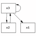
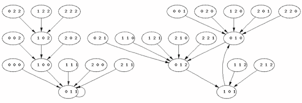
Figure 1. Wiring diagram (top) and state space (bottom) for the polynomial model $F$ in Example 3.3.

While the above polynomial dynamical system may be a reasonable model for the 3-gene network, it is not unique. We recall from Theorem 2.2 that the number of monomials in the basis for $k[x_{1},x_{2},x_{3}]/I(\mathbf{p}_{1},\ldots,\mathbf{p}_{4})$ is the number of data points (4, in this case). Since any transition function can be written as a $k$-linear combination of the basis monomials, then for a fixed term order there are $|k|^{m}=3^{4}$ possible transition functions where $m$ is the number of data points. In fact there are $(|k|^{m})^{n}=3^{12}$ possible polynomial models, given a term order. As there are 5 term orders which produce distinct polynomial models , there are $((|k|^{m})^{n})^{5}=3^{60}$ possible models for a 3-variable system on 3 states and 4 data points.

An important problem in this context that is common to both design of experiments and biochemical network inference is the construction of good fractional designs that narrow down the model space as much as possible. The challenge in network inference is that experimental observations tend to be very costly, severely limiting the number of points one can collect. Furthermore, many points are impossible to generate biologically or experimentally, which provides an additional constraint on the choice of fractional design.

4. Polynomial dynamical systems

It is worth mentioning that polynomial dynamical systems over finite fields (not to be confused with dynamical systems given by differential equations in polynomial form) have been studied in several different contexts. For instance, they have been used to provide state space models for systems for the purpose of developing controllers ML1 ; ML2 in a variety of contexts, including biological systems JVDL . Another use for polynomial dynamical systems is as a theoretical framework for agent-based computer simulations LJMR . Note that this class of models includes cellular automata and Boolean networks (choosing the field with two elements as state set), so that general polynomial systems are a natural generalization. In this context, an important additional feature is the update order of the variables involved.

The dynamical systems in this paper have been updated in parallel, in the following sense. If $f=(f_{1},\ldots,f_{n})$ is a polynomial dynamical system and $\mathbf{a}\in k^{n}$ is a state, then $f(\mathbf{a})=(f_{1}(\mathbf{a}),\ldots,f_{n}(\mathbf{a}))$. By abuse of notation, we can consider each of the $f_{i}$ as a function on $k^{n}$ which only changes the $i$th coordinate. If we now specify a total order of $1,\ldots,n$, represented as a permutation $\sigma\in S_{n}$, then we can form the dynamical system

$$f_{\sigma}=f_{\sigma(n)}\circ f_{\sigma(n-1)}\circ\cdots\circ f_{\sigma(1)},$$

which, in general, will be different from $f$. Thus, $f_{\sigma}$ is obtained through sequential update of the coordinate functions. Sequential update of variables plays an important role in computer science, e.g., in the context of distributed computation. See LJMR for details.

Many processes that can be represented as dynamical systems are intrinsically stochastic, and polynomial dynamical systems can be adapted to account for this stochasticity. In the context of biochemical network models, sequential update order arises naturally through the stochastic nature of biochemical processes within a cell that affects the order in which processes finish. This feature can be incorporated into polynomial dynamical system models through the use of random sequential update. That is, at each update step a sequential update order is chosen at random. It was shown in cas05 in the context of Boolean networks that such models reflect the biology more accurately than parallel update models. In Shmulevich:02b a stochastic framework for gene regulatory networks was proposed which introduces stochasticity into Boolean networks by choosing at each update step a random coordinate function for each variable, chosen from a probability space of update functions. Stochastic versions of polynomial dynamical systems have yet to be studied in detail and many interesting problems arise that combine probability theory, combinatorics, and dynamical systems theory, providing a rich source of cross-fertilization between these fields.

5. Discussion

This paper focuses on polynomial models in two fields, design of experiments and inference of biochemical networks. We have shown that the problem of inferring a biochemical network from a collection of experimental observations is a problem in the design of experiments. In particular, the question of an optimal experimental design for the identification of a good model is of considerable importance in the life sciences. When focusing on gene regulatory networks, it has been mentioned that conducting experiments is still very costly, so that the size of a fractional design is typically quite small compared to the number of factors to be considered. Another constraint on experimental design is the fact that there are many limits to an experimental design imposed by the biology, in particular the limited ways in which a biological network can be perturbed in meaningful ways. Much research remains to be done in this direction.

An important technical issue we discussed is the dependence of model choices on the term order used. In particular, the term order choice affects the wiring diagram of the model which represents all the causal interaction among the model variables. Since there is generally no natural way to choose a term order this dependence cannot be avoided. We have discussed available modifications that do not depend on the term order, at the expense of only producing a wiring diagram rather a dynamic model. This issue remains a focus of ongoing research.

As one example, an important way to collect network observations is as a time course of measurements, typically at unevenly spaced time intervals. The network is perturbed in some way, reacts to the perturbation, and then settles down into a steady state. The time scale involved could be on the scale of minutes or days. Computational experiments suggest that, from the point of view of network inference, it is more useful to collect several shorter time courses for different perturbations than to collect one highly resolved time course. A theoretical justification for these observations would aid in the design of time courses that optimize information content of the data versus the number of data points.

6. Acknowledgements

Laubenbacher was partially supported by NSF Grant DMS-0511441 and NIH Grant R01 GM068947-01. Stigler was supported by the NSF under Agreement No. 0112050.

Appendix A Concepts from computational algebra

In this section, we let $k$ denote a field and $R$ the polynomial ring $k[x_{1},\ldots,x_{n}]$. A subset $I\subset R$ is an ideal if it is closed under addition and under multiplication by elements of $R$.

Definition A.1.

Let $V$ be a finite set of points in $k^{n}$. The set

$$\mathbf{I}(V)=\{f\in R:f(a)=0\text{ for all }a\in V\}$$

of polynomials that vanish on $V$ is called the ideal of points of $V$.

Note that $\mathbf{I}(V)$ is indeed an ideal. In fact, $\mathbf{I}(V)$ is zero-dimensional since the $k$-vector space $R/\mathbf{I}(V)$ is finite dimensional with $dim_{k}(R/\mathbf{I}(V))=|V|$. While the number of generators of the vector space is fixed, the generators themselves depend on the choice of term order.

Definition A.2.

A term order on $R$ is a relation $\succ$ on the set of monomials $\mathbf{x}^{a}:=x_{1}^{a_{1}}x_{2}^{a_{2}}\cdots x_{n}^{a_{n}}$ such that $\succ$ is a total ordering,

$$\mathbf{x}^{a}\succ\mathbf{x}^{b}\implies\mathbf{x}^{a}\mathbf{x}^{c}\succ\mathbf{x}^{b}\mathbf{x}^{c}$$

for any monomial $\mathbf{x}^{c}$, and $\succ$ is a well-ordering; i.e., every nonempty subset of monomials has a smallest element under $\succ$.

Given a term order $\succ$, every nonzero polynomial $f\in R$ has a canonical representation as a formal sum of monomials

$$f=\sum_{i=1}^{r}a_{i}f_{i}$$

with $f_{i}\in R$ and $a_{i}\in k$ for $i=1,\ldots,r$, and $a_{i}f_{i}\succ a_{j}f_{j}$ for all $i>j$. Moreover, $a_{1}f_{1}$ is called the leading term of $f$.

Definition A.3.

Let $\succ$ be a term order and $I\subset R$ an ideal. A finite subset $G=\{g_{1},\ldots,g_{m}\}\subset I$ is a Gröbner basis for $I$ if the leading term of any $f\in I$ is divisible by the leading term of some $g_{i}$ under $\succ$. The normal form of $f\in R$ with respect to $G$, denoted $NF(f,G)$, is the remainder of $f$ after division by the elements of $G$.

Theorem A.4.

Every nonzero ideal $I\subset R$ has a Gröbner basis.

Theorem A.5.

Let $G$ be a Gröbner basis for $I\subset R$ and let $f\in R$. Then $NF(f,G)$ is unique.

Let $G$ be a Gröbner basis and $LT(G)$ be the set of leading terms of the elements of $G$. The set $\{\mathbf{x}^{a}:\mathbf{x}^{a}\notin LT(G)\}$ is a basis for $R/\mathbf{I}(V)$ and its elements are called standard monomials. Given a Gröbner basis $G$ of $\mathbf{I}(V)$ with respect to a term order, every nonzero polynomial $\bar{f}\in R/\mathbf{I}(V)$ has a unique representation as a formal sum of the standard monomials.

References

- [1] M. Chaves, R. Albert, and E. Sontag, Robustness and fragility of boolean models for genetic regulatory networks, 235 (2005), pp. 431–449.
- [2] J. M. E. Dimitrova, P. Vera-Licona and R. Laubenbacher, Comparison of data discretization methods for inference of biochemical networks. 2007.
- [3] A. Jarrah, H. Vastani, K. Duca, and R. Laubenbacher, An optimal control problem for in vitro virus competition, in 43rd IEEE Conference on Decision and Control, 2004.
- [4] R. Laubenbacher and B. Stigler, A computational algebra approach to the reverse engineering of gene regulatory networks, Journal of Theoretical Biology, 229 (2004), pp. 523–537.
- [5] H. Marchand and M. LeBorgne, On the optimal control of polynomial dynamical systems over , in Fourth Workshop on Discrete Event Systems, IEEE, Cagliari, Italy, 1998.
- [6] , Partial order control of discrete event systems modeled as polynomial dynamical systems, in IEEE International conference on control applications, Trieste, Italy, 1998.
- [7] G. Pistone, E. Riccomagno, and H. P. Wynn, Algebraic Statistics, Chapman&Hall, Boca Raton, FL, 2001.
- [8] G. Pistone and H. P. Wynn, Generalized confounding with Gröbner bases, Biometrika, 83 (1996), pp. 653–666.
- [9] H. M. R. Laubenbacher, A. S. Jarrah and S. Ravi, A mathematical formalism for agent-based modeling, in Encyclopedia of Complexity and Systems Science, R. Meyers, ed., Springer Verlag, 2009.
- [10] E. Riccomagno, Algebraic geometry in experimental design and related fields, PhD thesis, Dept. of Statistics, University of Warwick, 1997.
- [11] L. Robbiano, Gröbner bases and statistics, in Gröbner Bases and Applications (Proc. of the Conf. 33 Years of Gröbner Bases), B. Buchberger and F. Winkler, eds., vol. 251 of London Mathematical Society Lecture Notes Series, Cambridge University Press, 1998, pp. 179–204.
- [12] I. Shmulevich, E. R. Dougherty, S. Kim, and W. Zhang, Probabilistic boolean networks: A rule-based uncertainty model for gene regulatory networks, Bioinformatics, 18 (2002), pp. 261–274.