Perturbative fragmentation

Abstract

The Berger model of perturbative fragmentation of quarks to pions berger is improved by providing an absolute normalization and keeping all terms in a $(1-z)$ expansion, which makes the calculation valid at all values of fractional pion momentum $z$. We also replace the nonrelativistic wave function of a loosely bound pion by the more realistic procedure of projecting to the light-cone pion wave function, which in turn is taken from well known models. The full calculation does not confirm the $(1-z)^{2}$ behavior of the fragmentation function (FF) predicted in berger for $z>0.5$, and only works at very large $z>0.95$, where it is in reasonable agreement with phenomenological FFs. Otherwise, we observe quite a different $z$-dependence which grossly underestimates data at smaller $z$. The disagreement is reduced after the addition of pions from decays of light vector mesons, but still remains considerable. The process dependent higher twist terms are also calculated exactly and found to be important at large $z$ and/or $p_{T}$.

I Introduction

The fragmentation of colored partons, quarks and gluons, into colorless hadrons is an essential ingredient of any semi-inclusive hadronic reaction, since confinement does not allow propagation of free color charges. For this reason hadronization is usually considered to be related necessarily to confinement specific to the string model cnn . Indeed, the string model of hadron production is rather successful in describing data.

In a typical event of quark fragmentation the mean production time $t_{p}$ of a pre-hadron (i.e. a colorless cluster developing afterwards a corresponding wave function) linearly rises with its energy, and the most energetic hadron in such event takes about half of the initial quark energy. In some rare events, however, the leading hadron may take the main fraction $z\to 1$ of the initial quark energy. This process cannot last long, since the leading quark is constantly losing momentum, $dp_{q}/dt=-\kappa$, where $\kappa$ is the string tension. Therefore the production time should shrink at $z\to 1$ as kn ,

$$t_{p}=(1-z)\,\frac{E_{q}}{\kappa}\,.$$ (1)

Notice that the end-point behavior of the production time, $t_{p}\propto(1-z)$, is not specific for the string model, but is a result of energy conservation.

The shortness of the production time is an indication that a nonperturbative approach for the production of hadrons with large $z\to 1$ is not really required. Indeed, according to (1), in this region the hadronization time shrinks, i.e. the quark directly radiates a hadron, $q\to h+q$. Furthermore, since the invariant mass squared of the final state is $M_{qh}^{2}=m_{h}^{2}/z+m_{q}^{2}/(1-z)+p_{T}^{2}/z(1-z)$, where $p_{T}$ is the transverse hadron momentum, at $z\to 1$ the initial quark is far off mass shell, and this process can be treated perturbatively. This observation motivates a perturbative QCD calculations for leading pion production $q\to\pi q$, within the model proposed by Berger berger , as is illustrated in Fig. 1 for $l\bar{l}$ annihilation.

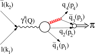
Figure 1: $l\bar{l}$ annihilation with production of two $\bar{q}q$ pairs. The large blob contains gluon radiation by either $\bar{q}_{1}$ or $q_{2}$. Four-momenta of particles are shown in parentheses.

He found that the fragmentation function of a quark to a pion vanishes as $(1-z)^{2}$ at $z\to 1$, and falls as function of transverse pion momentum as $1/p_{T}^{4}$. Besides, a nonfactorizable, scaling violating term was found to dominate at $z\to 1$. The shape of $z$-dependence calculated by Berger berger was found to agree well with data after the inclusion of gluon radiation cf. Ref. kpps .

Unfortunately, the calculation performed in berger missed the absolute normalization of the cross section, which makes it difficult to compare with data. Moreover, it was done in lowest order in $(1-z)$, therefore it is not clear in which interval of $z$ the model is realistic. And last, but not least, the calculations were based on the nonrelativistic approximation for the pion structure function, assuming equal sharing of longitudinal and transverse momenta by the quark and antiquark in the pion. However, the dominant configuration of the $\bar{q}q$ pair projected to the pion is asymmetric, with the projectile quark carrying the main fraction of the momentum.

Here we perform calculations first in the Berger approximation, but retaining the absolute normalizations and higher powers of $(1-z)$ (Sect. 3). Then, in Sect. 4 we give up the nonrelativistic approximation and project the amplitude of $\bar{q}q$ production onto the light-cone (LC) wave function of the pion. For this wave function we consider three different models and find reasonable agreement with phenomenological fragmentation functions (FF), but only at large $z>0.95$. To improve agreement at smaller $z$ we add pions originating from decays of $\rho$ and $\omega$ mesons, which are produced by the same mechanism, and which is depicted in Fig. 1. In Sect. 5 we study higher twist contributions, which gives a sizeable contribution in semi-inclusive pion production in DIS at moderately large $Q^{2}$ and large $z$.

II Leading hadrons in Born approximation

The amplitude of the process $l\bar{l}\to\bar{q}_{1}+q_{2}+G\to\bar{q}_{1}+q_{2}+\bar{q}_{3}+q_{4}$, depicted in Fig. 1, in the lowest order of pQCD is given by,

$$A(l\bar{l}\to\bar{q}_{1}q_{2}\bar{q}_{3}q_{4})={1\over Q^{2}}\,J_{\mu}^{(l)}(k_{1},\bar{\lambda}_{1};k_{2},\bar{\lambda}_{2})$$ (2)

$$\times J_{\mu}^{(h)}(p_{1},\lambda_{1},i_{1};p_{2},\lambda_{2},i_{2};p_{3},\lambda_{3},i_{3};p_{4},\lambda_{4},i_{4}).$$

Here $k_{1},\bar{\lambda}_{1}$ and $k_{2},\bar{\lambda}_{2}$ are 4-momenta and helicities of the lepton and antilepton respectively; $p_{l},\ \lambda_{l}$ and $i_{l}$ are the 4-momenta, helicities and color indexes of the quarks $q_{1}$ and $q_{3}$ ($l=1,3$) and antiquarks $\bar{q}_{2}$ and $\bar{q}_{4}$ ($l=2,4$). The 4-momentum $Q=k_{1}+k_{2}$.

The leptonic and hadronic currents in (2) read,

$$J_{\mu}^{(l)}(k_{1},\bar{\lambda}_{1};k_{2},\bar{\lambda}_{2})=e\,\bar{u}_{\bar{\lambda}_{2}}(k_{2})\gamma_{\mu}v_{\bar{\lambda}_{1}}(k_{1})\,;$$ (3)

$$J_{\mu}^{(h)}(p_{1},\lambda_{1},i_{1};p_{2},\lambda_{2},i_{2};p_{3},\lambda_{3},i_{3};p_{4},\lambda_{4},i_{4})$$ (4)

$$= {1\over M^{2}}\,\sum\limits_{a=1}^{8}{g_{s}\over 2}\,\lambda^{(a)}_{i_{2}i_{1}}{g_{s}\over 2}\,\lambda^{(a)}_{i_{4}i_{3}}$$

$$\times T_{\mu\nu}(p_{1}\lambda_{1},p_{2}\lambda_{2})\,j_{\nu}(p_{3}\lambda_{3},p_{4}\lambda_{4})\,.$$

Here $M^{2}=(p_{3}+p_{4})^{2}$ is the gluon invariant mass squared; $g_{s}^{2}=4\pi\alpha_{s}$; $\lambda^{(a)}_{ij}$ are Gell-Mann matrices;

$$T_{\mu\nu}(p_{1}\lambda_{1},p_{2}\lambda_{2}) = e_{q_{1}}\,\bar{u}_{\lambda_{2}}(p_{2})\,\bigl{[}\gamma_{\mu}\hat{G}(Q-p_{1})\gamma_{\nu}$$ (5)

$$+ \gamma_{\nu}\hat{G}(p_{2}-Q)\gamma_{\mu}\bigr{]}\,v_{\lambda_{1}}(p_{1})\,,$$

where $\hat{G}(q)=(\hat{q}+m_{q})/(q^{2}-m_{q}^{2})$; $\hat{q}=q_{\mu}\gamma_{\mu}$; $m_{q}$ is the quark mass; and

$$j_{\nu}(p_{3}\lambda_{3},p_{4}\lambda_{4})=\bar{u}_{\lambda_{4}}(p_{4})\,\gamma_{\nu}\,v_{\lambda_{3}}(p_{3})\,.$$ (6)

III Berger model

In the Berger model berger the amplitude $\tilde{A}$ of the reaction $l\bar{l}\to\pi q_{1}q_{4}$ is a result of projection of the amplitude Eq. (2) on the $S$-wave colorless state of the $q_{2}\bar{q}_{3}$ pair having zero total spin. The result of the projection is proportional to $\Psi_{\pi}(\vec{r}=0)$ ($\vec{r}$ is 3-dimensional) with a pre-factor $\sqrt{2/m_{\pi}}$ nemenov , where $m_{\pi}$ is the pion mass. Then we get,

$$\tilde{A}(l\bar{l}\to\pi q_{1}q_{4})={1\over Q^{2}}\,J_{\mu}^{(l)}\,\bar{J}_{\mu}^{(h)}\,\sqrt{2\over m_{\pi}}\,\Psi_{\pi}(0)\,.$$ (7)

Here

$$\bar{J}_{\mu}^{(h)}=\frac{1}{\sqrt{3}}\sum\limits_{i=1}^{3}\frac{1}{\sqrt{2}}\sum\limits_{\lambda=\pm 1/2}{\rm sgn}(\lambda)$$ (8)

$$\times J_{\mu}^{(h)}(p_{1},\lambda_{1},i_{1};p,\lambda,i;p,-\lambda,i;p_{4},\lambda_{4},i_{4})\,,$$

and the summations $\frac{1}{\sqrt{3}}\sum_{i=1}^{3}$ and $\frac{1}{\sqrt{2}}\sum_{\lambda=\pm 1/2}{\rm sgn}(\lambda)$ perform projections to colorless and spinless states of the $q_{2}\bar{q}_{3}$ pair, respectively.

Then we can make use of the relations,

$$\sum\limits_{a=1}^{8}\sum\limits_{i_{1}}^{3}\lambda^{a}_{i_{4}i}\lambda^{a}_{ii_{1}} = {16\over 3}\,\delta_{i_{4}i_{1}}\,;$$

$$\sum\limits_{\lambda=\pm 1/2}{\rm sgn}(\lambda)v_{-\lambda}(p_{4})\bar{u}_{\lambda}(p_{3})\Bigr{|}_{p_{3}=p_{4}\equiv p} = \gamma_{5}(\hat{p}+m),$$

and arrive at the following form of the hadronic current,

$$\bar{J}_{\mu}^{(h)}=\frac{2g_{s}^{2}e_{q_{1}}}{3\sqrt{6}\,M^{2}}\,(j_{1\mu}+j_{2\mu})\,,$$ (10)

where

$$j_{1\mu} = \bar{u}_{\lambda_{4}}(p_{4})\,\gamma_{\nu}\gamma_{5}(\hat{p}+m_{q})\gamma_{\nu}\hat{G}(Q-p_{1})\gamma_{\mu}\,v_{\lambda_{1}}(p_{1})$$ (11)

$$= \bar{u}_{\lambda_{4}}(p_{4})\,\gamma_{5}\left(\gamma_{\mu}-\frac{2m_{q}\hat{p}\,\gamma_{\mu}}{M^{2}}\right)\,v_{\lambda_{1}}(p_{1})\,;$$

$$j_{2\mu} = \bar{u}_{\lambda_{4}}(p_{4})\,\gamma_{\nu}\gamma_{5}(\hat{p}+m_{q})\gamma_{\mu}\hat{G}(p_{2}-Q)\gamma_{\nu}\,v_{\lambda_{1}}(p_{1})$$ (12)

$$= \frac{4}{Q^{2}-2pQ}\,\bar{u}_{\lambda_{4}}(p_{4})\,\gamma_{5}\Bigl{[}(p_{1}p+m_{q}^{2})\gamma_{\mu}$$

$$- (p_{1\mu}+p_{\mu})\hat{p}-m_{q}\hat{p}\,\gamma_{\mu}+m_{q}Q_{\mu}\Bigr{]}\,v_{\lambda_{1}}(p_{1})\,.$$

Here we applied the algebra of $\gamma$-matrices, the Dirac equation and 4-momentum conservation, $Q=p_{1}+2p+p_{4}$. The invariant gluon mass $M$ was defined in (4).

It is convenient to choose the $z$-axis along the momentum $\vec{p}_{1}$ in the collision c.m. frame, and to switch from Lorentz 4-vectors $a_{\mu}$ (e.g. $J_{\mu}^{(l,h)},\ p_{\mu 1},\ p_{\mu 4},\ Q_{\mu},\ etc.$) to light-cone vectors, $(a_{+},a_{-},\vec{a}_{\perp})$, where $a_{\pm}=a_{0}\pm a_{z}$. Since $\vec{Q}=0$, i.e. $Q_{+}=Q_{-}$, the condition of gauge invariance, $Q_{\mu}J^{(l)}_{\mu}=Q_{\mu}\bar{J}^{(h)}_{\mu}=0$, takes the form, $J^{(l)}_{+}=-J^{(l)}_{-}$ and $\bar{J}^{(h)}_{+}=-\bar{J}^{(h)}_{-}$. Then the product of the lepton and hadronic currents can be presented as,

$$J^{(l)}_{\mu}\bar{J}^{(h)}_{\mu}=-J^{(l)}_{+}\bar{J}^{(h)}_{+}-J^{(l)}_{\perp}\bar{J}^{(h)}_{\perp}\,.$$ (13)

The typical values of transverse components are $|\vec{p}_{\perp}|\sim m_{q}$, $\vec{p}_{4T}=-2\vec{p}$, $\left|\vec{J}^{(l)}_{\perp}\right|\sim J^{(l)}_{+}$, so

$$\bar{J}^{(h)}_{+}\sim{m_{q}\over Q}\left|\vec{J}^{(h)}_{\perp}\right|$$ (14)

Therefore, the first term in (13) can be safely neglected. Then we get,

$$\bar{J}^{(h)}_{\perp} = \frac{4g_{s}^{2}e_{q_{1}}\delta{i_{4}i_{1}}}{3\sqrt{6}\,M^{2}}\,\bar{u}(p_{4})\,\gamma_{5}$$ (15)

$$\times \left[\xi\,\gamma_{\perp}-\frac{2m_{q}}{M^{2}}\,\hat{p}\gamma_{\perp}\right]\,v(p_{1})\,,$$

where $\xi=(2+z)/(2-z)$, and

$$z=\frac{p_{\pi+}}{Q_{+}}=\frac{2p_{+}}{Q_{+}}\,,$$ (16)

is the fractional pion momentum. In this approximation the invariant gluon mass reads,

$$M^{2}=(p+p_{4})^{2}=2\,\frac{m_{q}^{2}(1-z/2)^{2}+\vec{p}_{\perp}^{2}}{z(1-z)}\,.$$ (17)

Notice that although the second term in (15) is proportional to the quark mass (which was assumed in berger to be zero), it should not be neglected. Indeed, after integration over $\vec{p}_{T}$ the interference of the two terms in (15) is of the same order as the first term squared.

In this approximation the fragmentation function gets the form,

$$D_{q}^{\pi}(z) = \frac{64\alpha_{s}^{2}}{27m_{\pi}m_{q}^{2}}\,\left|\Psi_{\pi}(0)\right|^{2}\,\frac{z(1-z)^{2}}{(2-z)^{2}}$$

$$\times \left[\xi^{2}+2(\xi+1)\left(\frac{z}{2-z}\right)^{2}-{16\over 3}\,\frac{z^{2}(1-z)}{(2-z)^{4}}\right].$$

The pion wave function at the origin correlates with the shape of the parametrization for $\Psi_{\pi}(r)$. In the case of a Gaussian parametrization,

$$\left|\Psi_{\pi}(\vec{r})\right|^{2}_{gauss}=\frac{\kappa_{1}^{3}}{\pi^{3/2}}\exp(-\kappa_{1}^{2}r^{2}/2)\,,$$ (19)

the pion form factor has the form, $F_{\pi}(q^{2})=\exp(-q^{2}/16\kappa_{1}^{2})$. So $\kappa_{1}^{2}=3/8\langle r_{ch}^{2}\rangle$.

With a bit more realistic exponential shape,

$$\left|\Psi_{\pi}(\vec{r})\right|^{2}_{exp}=\frac{\kappa_{2}^{3}}{\pi^{2}}\exp(-2\kappa_{2}r)\,,$$ (20)

the pion form factor reads, $F_{\pi}(q^{2})=\left(1+q^{2}/16\kappa_{2}^{2}\right)^{-2}$. Then $\kappa_{2}^{2}=2\kappa_{1}^{2}$.

These two examples demonstrate the high sensitivity of the wave function at the origin to the choice of $r$-dependence. One finds $|\Psi_{\pi}(0)|^{2}_{exp}/|\Psi_{\pi}(0)|^{2}_{gauss}=\sqrt{8\pi}\approx 5$. Therefore, it is difficult to conclude whether the Berger model agrees or not with data.

Another, more realistic option would rely on the pole form of the pion form factor, $F_{\pi}(q^{2})=\kappa_{3}^{2}/(\kappa_{3}^{2}+q^{2})$, where $\kappa_{3}^{2}=1/6\langle r_{ch}^{2}\rangle$. Then,

$$\left|\Psi_{\pi}(\vec{r})\right|^{2}=\frac{1}{r}\exp(-\kappa_{3}r)\,.$$ (21)

In this case, however, the wave function at the origin is divergent.

The Berger approximation, assuming that the pion production amplitude is proportional to the amplitude of $\bar{q}q$ production with equal momenta, would be justified if the pion was a nonrelativistic, loosely bound system, i.e. $m_{\pi}\approx 2m_{q}$, $2m_{q}-m_{\pi}\ll m_{q}$. However, the mean charge radius squared is much smaller than the value given by such a nonrelativistic model, $\langle r_{ch}^{2}\rangle=(4m_{q}^{2}-m_{\pi}^{2})^{-1}$.

On the other hand, a description of the pion as a relativistic bound system has been a challenge so far.

IV Projection to the LC wave function

IV.1 Direct pions

In the light-cone (LC) representation the pion wave function depends on the fractional LC momenta of the quark, $\alpha=p_{2+}/p_{\pi+}$, and antiquark, $1-\alpha=p_{3+}/p_{\pi+}$, and the relative transverse momentum, $k_{\perp}=\alpha p_{3\perp}-(1-\alpha)p_{2\perp}$. In this representation the amplitudes, Eqs. (7) and (2), are related as,

$$\tilde{A}=\frac{1}{(2\pi)^{3}}\int\limits_{0}^{1}\frac{d\alpha}{\sqrt{2\alpha(1-\alpha)}}\int d^{2}k_{\perp}\,A(\alpha,k_{\perp})\,\Psi_{\pi}(\alpha,k_{\perp})\,,$$ (22)

where the $\bar{q}q$ Fock component of the pion LC wave function is normalized to unity,

$$\int\limits_{0}^{1}d\alpha\int d^{2}k_{\perp}\,\left|\Psi_{\pi}(\alpha,k_{\perp})\right|^{2}=1\,.$$ (23)

In this case the projection of the distribution amplitude of $q_{2}$ and $\bar{q}_{3}$ on the pion LC wave function is more complicated that in Berger model ($\alpha=1/2$), however it can be grossly simplified if one neglects small terms of the order of $m$ and $k_{\perp}$ in comparison with large $p_{2+}$ and $p_{3+}$ order terms. Then the combination in Eq. (LABEL:220) gets the simple form,

$$\sum\limits_{\lambda=\pm 1/2}{\rm sgn}(\lambda)\,v_{-\lambda}(p_{3})\bar{u}_{\lambda}(p_{2})=\gamma_{5}\,\hat{p}_{\pi}+O(m,k_{\perp})\,.$$ (24)

Furthermore, neglecting small terms we arrive at a new relation for the hadronic current of Eq. (15),

$$\bar{J}^{(h)}_{\perp}=\frac{8g_{s}^{2}e_{q_{1}}\delta{\alpha_{4}\alpha_{1}}}{3\sqrt{6}\,M^{2}}\,\frac{1+(1-\alpha)z)}{1-\alpha z}\,\bar{u}(p_{4})\gamma_{5}\gamma_{\perp}v(p_{1}).$$ (25)

When the momentum fractions of the quark and antiquark in the pion wave function are $\alpha$ and $1-\alpha$, then the invariant mass squared reads,

$$M^{2}=\frac{m^{2}(1-\alpha z)^{2}+[(1-\alpha)\vec{p}_{\pi\perp}-(1-z)\vec{k}_{\perp}]^{2}}{z(1-z)(1-\alpha)}\,.$$ (26)

The light-cone pion wave function can be parametrized as

$$\Psi_{\pi}(\alpha,\vec{r})=\phi(\alpha)\psi(r,\alpha)\,.$$ (27)

If the wave function in momentum representation has a monopole form, $\Psi_{\pi}(\alpha,k)\propto[k^{2}/\alpha(1-\alpha)+\kappa^{2}]^{-1}$, then

$$\psi(r,\alpha)=N\,K_{0}(\kappa r\sqrt{\alpha(1-\alpha)}),$$ (28)

where $K_{0}$ is the modified Bessel function. Since the momentum dependence of $\Psi_{\pi}(\alpha,k)$ is poorly known, we also performed calculations with a dipole dependent wave function in the Appendix, since comparison of the results shows the scale of the theoretical uncertainty.

The parameter $\kappa$ is fixed by the condition,

$$-\frac{dF_{\pi}(q)}{dq^{2}}\Bigr{|}_{q^{2}=0}={1\over 6}\,\langle r_{ch}^{2}\rangle\approx 1.83\,\mbox{GeV}^{-2},$$ (29)

where the pion form factor reads,

$$F_{\pi}(q)=\int d^{2}r\int\limits_{0}^{1}d\alpha|\Psi_{\pi}(\alpha,\vec{r})|^{2}\,e^{i\alpha\vec{q}\cdot\vec{r}}\,.$$ (30)

Thus, the parameter $\kappa$ as well as the normalization constant $N$ in (27) depend on the choice of function $\phi(\alpha)$. We consider two popular models (compare with dijet ):

Model 1: Standard (asymptotic) shape asymp ; radyushkin ,

$$\phi_{1}(\alpha) = \alpha(1-\alpha)\,;$$ (31)

$$N_{1}^{2} = \frac{6\kappa_{1}^{2}}{\pi}\,;$$

$$\kappa_{1}^{2} = \frac{2}{\langle r_{ch}^{2}\rangle}\,.$$ (32)

Model 2: Chernyak-Zhitnitsky model ch-zh ,

$$\phi_{2}(\alpha) = \phi_{1}(\alpha)\,(1-2\alpha)^{2}\,;$$ (33)

$$N_{2}^{2} = \frac{70\kappa_{2}^{2}}{\pi}\,;$$

$$\kappa_{2}^{2} = \frac{6}{\langle r_{ch}^{2}\rangle}\,.$$ (34)

To be specific we will calculate $D_{u}^{\pi^{+}}(p_{T}^{2},z)$ which is the FF of a $u$ quark into $\pi^{+}$. For the transverse momentum dependent fragmentation function we have for each of these versions (taking into account the longitudinal current contribution),

$$\left.\frac{dD_{u}^{\pi^{+}}(z,p_{T}^{2})}{dp_{T}^{2}}\right|_{i}=2\left(\frac{\alpha_{s}}{2\pi}\right)^{2}C_{i}\kappa_{i}^{2}z$$ (35)

$$\times \left[(1-z)^{2}\,F_{i}^{2}(z,p_{T})+\epsilon z^{2}\frac{4p_{T}^{2}}{Q^{2}}\,G_{i}^{2}(z,p_{T})\right]\,.$$

Here $i=1,\ 2$; $C_{1}=1$; $C_{2}=35/3$;

$$F_{i}(z,p_{T}) = \int\limits_{0}^{1}d\alpha\,\frac{(1-\alpha)\phi_{i}(\alpha)}{\sqrt{a_{i}^{2}-b_{i}}}\ \frac{1+(1-\alpha)z}{1-\alpha z}$$ (36)

$$\times \ln\left(\frac{a_{i}+\sqrt{a_{i}^{2}-b_{i}}}{a_{i}-\sqrt{a_{i}^{2}-b_{i}}}\right)\,;$$

$$G_{i}(z,p_{T}) = \int\limits_{0}^{1}d\alpha\,\frac{(1-\alpha)^{2}\phi_{i}(\alpha)}{(1-\alpha z)\sqrt{a_{i}^{2}-b_{i}}}\,$$ (37)

$$\times \ln\left(\frac{a_{i}+\sqrt{a_{i}^{2}-b_{i}}}{a_{i}-\sqrt{a_{i}^{2}-b_{i}}}\right)\,;$$

$$a_{i} = p_{T}^{2}(1-\alpha)^{2}+m_{q}^{2}(1-\alpha z)^{2}$$

$$+ \kappa_{i}^{2}\alpha(1-\alpha)(1-z)^{2}\,;$$

$$b_{i} = 4m_{q}^{2}\kappa_{i}^{2}(1-\alpha z)^{2}(1-z)^{2}\alpha(1-\alpha)\,.$$ (39)

In fact, only the first leading twist term in square brackets in (35) corresponds to the factorized FF. The second term is a higher twist term, whose value (factor $\epsilon$) is process dependent, and which is discussed in more detail in Sect. V below .

The results of the numerical calculations of the $p$-integrated FF, for each of the three models, are plotted as functions of $z$ in Fig. 2. The QCD coupling was fixed at $\alpha_{s}=0.4$.

Figure 2: The fragmentation function, Eq. (35), integrated over transverse momentum. Solid and dashed curves correspond to the models $1$ and $2$ for the pion LC wave function (see text) respectively.

The calculated fragmentation functions fall off with $z$ only at very large $z\to 1$, otherwise are rather flat, or even rise at small values of $z$. Such a behavior does not comply with data which suggest FF monotonically falling with $z$ florian . Apparently, the present calculations are missing some mechanisms contributing at small $z$.

IV.2 Vector meson decays

One of the processes contributing to the pion spectrum should be the production, by the same mechanism shown in Fig. 1, of heavier mesons which decay to pions. One of the most important corrections should come from $\rho$-meson production, which gives the following contribution

$$\Delta D_{u}^{\rho/\pi^{+}}(z)=\frac{1}{\sqrt{1-\xi}}\int\limits_{z_{min}}^{1}\frac{dz^{\prime}}{z^{\prime}}\,\left[D_{u}^{\rho^{+}}(z^{\prime})+D_{u}^{\rho^{0}}(z^{\prime})\right]\,.$$ (40)

The bottom integration limit reads,

$$z_{min} = 2z\,\frac{1-\sqrt{1-\xi}}{\xi}\,;$$

$$\xi = \frac{4m_{\pi}^{2}}{m_{\rho}^{2}}\,.$$ (41)

We assume that $D_{u}^{\rho^{+}}(z)=3D_{u}^{\pi^{+}}(z)$, since $\rho$ has spin 1, and that $D_{u}^{\rho^{0}}(z)={1\over 2}D_{u}^{\rho^{+}}(z)$.

The $\omega$-meson production may also be important. Pions from $\omega$ decays should be even softer because of the three-particle phase space. The corresponding correction to the pion spectrum can be calculated as follows.

$$\Delta D_{u}^{\omega/\pi^{+}}(z)=\frac{\int_{2m_{\pi}}^{m_{\omega}-m_{\pi}}dM_{2\pi}\,g(M_{2\pi})\,I(z,M_{2\pi})}{\int_{2m_{\pi}}^{m_{\omega}-m_{\pi}}dM_{2\pi}\,g(M_{2\pi})}\,,$$ (42)

where

$$g(M_{2\pi}) = \sqrt{(M_{2\pi}^{2}-4m_{\pi}^{2})\left(\Omega^{2}-4m_{\omega}^{2}m_{\pi}^{2}\right)}\,,$$

$$\Omega = m_{\omega}^{2}+m_{\pi}^{2}-M_{2\pi}^{2}\,;$$ (43)

and

$$I(z,M_{2\pi})=\int\limits_{z_{1}}^{z_{2}}\frac{dz^{\prime}}{z^{\prime}}\,D_{u}^{\omega}(z^{\prime})\,,$$ (44)

$$z_{1} = {\rm min}\left\{1,\ \frac{2m_{\omega}^{2}\,z}{\Omega+\sqrt{\Omega^{2}-4m_{\omega}^{2}m_{\pi}^{2}}}\right\}\,,$$

$$z_{2} = {\rm min}\left\{1,\ z\,\frac{\Omega+\sqrt{\Omega^{2}-4m_{\omega}^{2}m_{\pi}^{2}}}{2m_{\pi}^{2}}\right\}\,.$$ (45)

We assume that $D_{u}^{\omega}(z)=D_{u}^{\pi^{+}}(z)$, since the factor of 3 coming from spin enhancement is compensated by an isospin suppression.

Fig. 3 shows our results for $D_{u}^{\pi^{+}}(z)$ (dashed-dotted), $\Delta D_{u}^{\rho/\pi^{+}}(z)$ and $\Delta D_{u}^{\omega/\pi^{+}}(z)$ (dotted), and their sum (solid). We also plotted the phenomenological $D_{u}^{\pi^{+}}(z)$ (dashed) obtained from a global fit to data florian .

Figure 3: Comparison of the Model 1 (asymptotic shape of the pion wave function) with data. The curves from bottom to top are: dotted: pions from $\omega$ and $\rho$ decays; dot-dashed: direct fragmentation to pions; solid: sum of the three previous contributions; dashed: phenomenological FF for charged pions florian fitted to data at scale $\mu^{2}=0.5\,\mbox{GeV}^{2}$.

As anticipated, the production of $\rho$ contributes to the softer part of the pion momentum distribution, and does not affect its hard part.

Other meson decays should pull the medium-$z$ part of $D_{u}^{\pi^{+}}(z)$ further up, but accurate calculation of all those contributions is still a challenge.

Notice that our results have no $Q^{2}$ evolution, since the calculations are done in Born approximation. Modification of the $z$-dependence by gluon radiation makes it softer, closer to data, generating also a $Q^{2}$ evolution. These corrections were studied within the Fock state representation in kpps .

The transverse momentum distribution of pions is given by Eq. (35). One cannot compare with data the mean value of $\langle p_{T}^{2}\rangle$ since it is poorly defined. Indeed, $F_{i}\sim\ln(p_{T})/p_{T}^{2}$ at high $p_{T}$ , so $\langle p_{T}^{2}\rangle$ is divergent and depends on the upper cutoff.

Instead, one should compare with data the $p_{T}$ dependence. Our results for the $p_{T}$-distribution of the FF, Eq. (35), is depicted in Fig. 4 for several values of $z$.

Figure 4: The transverse momentum dependent FF, $dD_{q}^{\pi}(z)/dp_{T}^{2}$, calculated with Eq. (35) and the Model 1 for the production of direct pions. Solid, dashed and dotted curves are calculated at $z=0.75,\ 0.85$ and $0.95$ respectively. Data from emc at $W^{2}>350\,\mbox{GeV}^{2}$ are renormalized for a better comparison with our results.

It might be too early to compare these results with data, since we did not include yet the gluon radiation, intrinsic motion of quarks in the target, and decays of heavier mesons. Nevertheless it is useful to check whether the calculated $p_{T}$ dependence is in a reasonable accord to data. Notice that the data depicted in Fig. 4 are integrated over a rather large $z$-bin, $0.4<z<1$. The latter causes a considerable mismatch in normalization (see Fig. 3), so we renormalized the data emc to be able to compare the shapes, which then are in reasonable agreement.

V Higher twist terms

The last term, in square brackets in Eq. (35), is a higher twist effect. It does not vanish at $z\to 1$, but is suppressed by powers of $Q$. We neglected corrections of the order of $\langle p_{T}^{2}\rangle/(zQ^{2})$, which are important only at small $z$.

This higher twist term breaks down the universality of the fragmentation function, since the factor $\epsilon$ depends on the process. For $e^{+}e^{-}$ annihilation it is given by,

$$\epsilon(l\bar{l}\to\pi\bar{q}_{1}q_{4})=\frac{sin^{2}\theta}{1+cos^{2}\theta}\,,$$ (46)

where $\theta$ is the angle between the direction of $l\bar{l}$ collision and momentum $\vec{p}_{1}$ in the c.m. frame.

For deep-inelastic scattering it reads,

$$\epsilon(lq_{1}\to l^{\prime}q_{4}\pi)=\frac{1-y}{2(1-y)+y^{2}}\,,$$ (47)

where $y=q_{+}/l_{+}$; $q_{\mu}$ is 4-momentum of the virtual photon; $l$ is 4-momentum of the initial lepton.

The relative contribution of the higher twist term is,

$$R_{i}(z,p_{T})=4\epsilon\,\left(\frac{z}{1-z}\right)^{2}\frac{p_{T}^{2}\,G_{i}^{2}(z,p_{T})}{Q^{2}\,F_{i}^{2}(z,p_{T})}\,,$$ (48)

where subscript $i$ denotes the number of the model used for the LC pion wave function, and $G_{i}$, $F_{i}$ are defined in (36)-(37).

While the relative value of the nonfactorizable higher twist term is expected to be vanishingly small in $l\bar{l}$ annihilation, it might be a sizeable effect in SIDIS, usually associated with medium to large values of $Q^{2}$. The relative correction, Eq. (48), is plotted in Fig. 5 as function of $p_{T}$, for $Q^{2}=2.5\,\mbox{GeV}^{2}$ and several fixed values of $z$.

Figure 5: The relative higher twist correction to the FF of a quark in DIS as function of transverse momentum for fixed values of $z=0.75,\ 0.95$, and $Q^{2}=2.5\,\mbox{GeV}^{2}$. The solid and dashed curves come from calculations with Model 1, Eq. (31). and Model 2, Eq. (33), respectively

Solid and dashed curve correspond to the models 1 and 2 for the LC pion wave function, respectively. Although the higher twist term is relatively small for forward fragmentation, it becomes a dominant effect at $p_{T}^{2}\mathrel{\hbox to0.0pt{\lower 4.0pt\hbox{\hskip 1.0pt$\sim$}\hss}\raise 1.0pt\hbox{$>$}}1\,\mbox{GeV}^{2}$.

The corresponding higher twist correction to the $p_{T}$-integrated FF reads,

$$R_{i}(z)=4\epsilon\,\frac{\langle p_{T}^{2}\rangle}{Q^{2}}\,\left(\frac{z}{1-z}\right)^{2}\frac{\int_{0}^{\infty}dp_{T}^{2}\,G_{i}^{2}(z,p_{T})}{\int_{0}^{\infty}dp_{T}^{2}\,F_{i}^{2}(z,p_{T})}\,,$$ (49)

The factor $\langle p_{T}^{2}\rangle$ is divergent and depends on experimental kinematic cuts. Therefore one should rely on its value specific for each experiment.

Apparently, a direct way to see the higher twist contribution in data is to study the $Q^{2}$ behavior of the FF. However, such data at sufficiently large $z$ are not available so far. Therefore, we try to extract the higher twist contribution from the $z$-dependence. To do so we first fit data at moderate values $z<0.65$ where we do not expect a sizeable higher-twist corrections, with the standard parametrization $D_{q}^{\pi}(z)=Nz^{\alpha}(1-z)^{\beta}$. We use data from the HERMES experiment hermes . We added the statistic and systematic errors in quadratures. The data are corrected by subtraction of the contribution from diffractive vector mesons, $\gamma^{*}p\to\pi p$, which is another higher twist contribution (see section VI). We found $\alpha=-1.24\pm 0.04,\ \beta=1.5\pm 0.07,\ N=0.88\pm 0.07$. The data divided by this fitted $z-dependence$ are depicted in In Fig. 6

Figure 6: Hermes data hermes for multiplicity of charged pions produced in DIS on a proton, corrected for decays of vector mesons. The data points are divided by the fit to the data at $z<0.65$ (see text). The curve corresponds to $R_{1}(z)+1$ calculated with Eq. (49) at $Q^{2}=2.5\,\mbox{GeV}^{2}$ and $\langle p_{T}^{2}\rangle=0.25\,\mbox{GeV}^{2}$.

We compare this data with the relative contribution of higher twists $R_{1}(z)$, Eq. (49), calculated at $Q^{2}=2.5\,\mbox{GeV}^{2}$ and with the measured value of $\langle p_{T}^{2}\rangle\approx 0.25\,\mbox{GeV}^{2}$ hermes . Our results agree with the data reasonable well.

An attempt to see the higher twist effects in nuclear attenuation data was made in pg . They found higher twist corrections of similar magnitude.

Notice that other sources of pions, like decays of heavier mesons produced via the same mechanism, are important for leading twist part. However, they also supply the cross section with higher-twist terms. Nevertheless, we assume that these corrections affect the ratio much less than the cross section.

VI Hints from triple-Regge phenomenology

The factorized part, Eq. (LABEL:400), of the cross section of pion production in $l\bar{l}$ annihilation, is the same as in deep-inelastic scattering (DIS), where it can be compared with the expectations of the triple-Regge description, illustrated in Fig. 7.

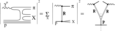
Figure 7: Virtual photoproduction of a pion via Reggeon exchange. The projectile quark from the photon fluctuation picks up an antiquark, produced either from the vacuum or perturbatively (see Fig. 1), and they form a pion.

The inclusive cross section at fixed $z$ is energy independent (Feynman scaling), and at fixed energy and $1-z\ll 1$ depends on $z$ as,

$$\frac{d\sigma(\gamma^{*}p\to\pi X)}{dz\,dp_{T}^{2}}\propto(1-z)^{n}\,,$$ (50)

where $z$ equals to Feynman $x_{F}$ in the triple-Regge kinematic region,

$$z\approx x_{F}=\left(1-\frac{M_{X}^{2}}{s}\right)(1-x_{Bj})\,,$$ (51)

and $x_{Bj}$ is the Bjorken variable.

The exponent in (50) is related to the parameters of the Regge trajectories involved,

$$n=1-2\alpha_{I\!\!R}(p_{T}^{2})\,.$$ (52)

Here $\alpha_{I\!\!R}(p_{T}^{2})$ is the trajectory of Reggeon ${I\!\!R}$. The rapidity interval, $\Delta y\approx-\ln(1-z)$, covered by the Reggeon is not large for the values of $z\sim 0.9$ under discussion. Therefore the pion Regge pole should dominate, since it has large coupling to nucleons. In this case, $\alpha_{\pi}(p_{T}^{2})\approx-\alpha^{\prime}_{\pi}p_{T}^{2}$, where $\alpha^{\prime}_{\pi}\approx 1\,\mbox{GeV}^{-2}$. Thus,

$$n_{\pi}=2\alpha^{\prime}_{\pi}\,\langle p_{T}^{2}\rangle\approx 1.5\,.$$ (53)

Here we rely on the value $\langle p_{T}^{2}\rangle\approx 0.25\,\mbox{GeV}^{2}$ measured in both HERMES hermes and EMC emc experiments. The value of the exponent given in Eq. (53) agrees quite well with data. Although our calculation confirmed the value $n=2$ found in berger , the inclusion of gluon radiation reduces the exponent $n$ down to the value observed in data kpps .

Notice that the $z$-dependence presented in Eqs. (50)-(52) changes at very small $1-z\ll 1$, and becomes rather flat. Indeed, we assumed that the invariant mass squared of the excitation $X$ is sufficiently large, $s(1-z)\gg m_{N}^{2}$ for the Pomeron to dominate in the bottom leg of the triple Regge graph in Fig. 7. However, this condition breaks down at very small $1-z$ and Reggeons with $\alpha_{I\!\!R}(0)=1/2$ dominate in the bottom leg. Another assumption we have made, pion dominance in the $t$-channel exchange, is also violated when the rapidity interval $\ln(1-z)$ becomes very large. Then Reggeons with a higher intercept $\alpha_{I\!\!R}(0)=1/2$ become the dominant contribution. Thus, the end-point behavior has the same power dependence, Eq. (50), but with a different exponent,

$$n(z\to 1)=\alpha_{I\!\!R}(0)-2\alpha_{I\!\!R}(p_{T}^{2})\approx-{1\over 2}+2\alpha^{\prime}_{I\!\!R}\,\langle p_{T}^{2}\rangle\approx 0\,.$$ (54)

Thus we arrive at the remarkable conclusion that the FF, which falls steeply with $z$, levels off at very small $1-z\ll 1$. This behavior, dictated by the triple-Regge formalism, is more general than perturbative calculations. One may wonder why this end-point feature is absent in our calculations. What has been missed? Notice that we did not care about the fate of the recoil quark $q_{4}$ in Fig. 1, which was justified by the condition of completeness. However, if the target excitation $X$ has a small invariant mass, it affects the probabilities of different final states of $q_{4}$.

The triple-Regge approach also indicates as an additional source of a higher twist contribution, which is specific for semi-inclusive DIS (SIDIS), the diffractive inclusive process $\gamma^{*}p\to\rho X$. The $p_{T}$-integrated cross section corresponding to the triple-Pomeron graph can be presented in the form,

$$\frac{d\sigma(\gamma^{*}p\to\rho X)}{dz} = \frac{G^{pp}_{3{I\!\!P}}(0)/2\alpha_{I\!\!P}^{\prime}}{(1-z)|\ln(1-z)|}\,\frac{16\pi}{(\sigma_{tot}^{pp})^{2}}$$ (55)

$$\times \left.\frac{d\sigma(\gamma^{*}p\to\rho p)}{dp_{T}^{2}}\right|_{p_{T}=0}\,,$$

where $G^{pp}_{3{I\!\!P}}(0)=3.2\,\mbox{mb}/\,\mbox{GeV}^{2}$ is the effective triple-Pomeron coupling, extracted from the fit kklp to data on $pp\to pX$. Here we neglected the transverse size of the $\bar{q}q$ dipole projected to $\rho$, since it is small, $1/Q^{2}$, and the $p_{T}$ dependence of the bare triple Pomeron vertex, since it is very weak spots . All the cross sections in (55) should be taken at a c.m. energy squared $s^{\prime}=s_{0}/(1-z)$, where $s_{0}=1\,\mbox{GeV}^{2}$.

The $z$-distribution of the produced $\rho^{0}$-mesons strongly peaks at $z\to 1$ (as any diffractive process should) and their decays feed the effective FF $D_{q}^{\pi}(z)$,

$$\left[\Delta D_{u}^{\rho/\pi^{+}}(z)\right]_{diff}=\frac{1}{\sigma^{\gamma^{*}p}_{tot}}\int\limits_{z_{min}}^{1}\frac{dz^{\prime}}{\sqrt{1-\xi}}\,\frac{d\sigma(\gamma^{*}p\to\rho^{0}X)}{z^{\prime}dz^{\prime}}\,.$$ (56)

Here $\xi$ and $z_{min}$ are defined in (41). Due to color transparency the amplitude of $rho$ production is inversely proportional to $Q^{2}$, therefore $\sigma(\gamma^{*}p\to\rho^{0}X)\propto 1/Q^{4}$. On the other hand, the total virtual photoabsorption cross section is $\sigma^{\gamma^{*}p}_{tot}\propto 1/Q^{2}$ (Bjorken scaling). Therefore, the diffractive contribution to the effective FF $q\to\pi$ is a higher twist effect, $\left[\Delta D_{u}^{\rho/\pi^{+}}(z)\right]_{diff}\propto 1/Q^{2}$.

The elastic production of vector mesons, $\gamma^{*}p\to Vp$ certainly also contributes to inclusive pion production, and is also a higher twist effect. It can be evaluated using Eq. (56) and a delta function for the $z^{\prime}$-distribution of produced vector mesons. However, in some cases, like in hermes , this contribution has been removed from data.

VII Summary

We performed calculations for the Berger perturbative mechanism berger of quark fragmentation into leading pions, keeping all the sub-leading terms in powers of $(1-z)$ and all the coefficients. Our results can be summarized as follows.

• We performed a full calculation of the quark FF including higher twist terms within the Berger approximation. However, we concluded that the approximation of a nonrelativistic pion wave function is unrealistic and brings too much uncertainty to the results of the calculation.

• We projected the produced $\bar{q}q$ pair distribution amplitude to the light-cone pion wave function. For the latter we employed two popular models: (i) the standard asymptotic shape (31); (ii) Model of Chernyak-Zhitnitsky (33). Both models lead to a $z$-dependence quite different from the one inferred from data. Only at $z\geq 0.95$ our calculations agree reasonably with data (both the shape and value), but greatly underestimate data at smaller values of $z$.

• Remarkably, the main amount of pions produced in quark fragmentation are not produced directly, except the most energetic ones with $z>0.95$. This fact should be taken into account in models employing perturbative hadronization knph

• Searching for ways of improving the description of data we added pions originated from decay of light vector mesons $\rho$ and $\omega$. Although this contribution pulled up the production of pions at medium to large $z$, apparently some contributions are still missing. That may be production and decays of heavier mesons, which are difficult to evaluate.

• We also performed a full calculation for the higher twist term originated from the longitudinal current contribution. It overcomes the leading twist term at large $z$ and/or large transverse momenta.

• A new higher twist contribution to pion production is found. It is related to decays of diffractively produced vector mesons.

It worth reminding that our results for the FF at large $z>0.9$ should be compared with a phenomenological one with precaution. First of all, data at such large $z$ are scarce and different parametrizations florian ; bkk ; kkp differ from each other considerably. Second of all, our FF is calculated in the Born approximation. Evolution (gluon radiation) may considerably change the shape of the $z$-dependence kpps .

Appendix A Dipole form of the pion LC wave function

Figure 8: Fragmentation functions for direct pions calculated with pole, Eq. (27) (solid curves), and dipole, Eq. (A.1) (dashed curves), parametrization for the transverse momentum dependent part of the LC pion wave function. Labels $1$ and $2$ indicate the model used for the longitudinal momentum dependence of the pion wave function.

To see the sensitivity to the form $r$-dependence of the LC wave function of the pion we also performed calculations with the dipole parametrization of transverse momentum dependent part of the LC wave function $\Psi_{\pi}(\alpha,\vec{k})\propto\left[\frac{k^{2}}{\alpha(1-\alpha)}+\kappa^{2}\right]^{-2}$. In impact parameter representation it takes the form (compare with (27)),

$$\Psi_{\pi}(\alpha,\vec{r})=N\,\phi(\alpha)\sqrt{\alpha(1-\alpha)}\,rK_{1}(\kappa r\sqrt{\alpha(1-\alpha)}),$$ (A.1)

In this case we can still employ Eq. (35) for the fragmentation function, but with a new form of function $F_{i}(z,p_{T})$,

$$F_{i}(z,p)=\int\limits_{0}^{1}d\alpha\,\frac{(1-\alpha)\phi_{i}(\alpha)}{a_{i}^{2}-b_{i}}\ \frac{1+(1-\alpha)z}{1-\alpha z}$$

$$\times \left[a_{i}-2d_{i}+\frac{d_{i}(a-2e_{i})}{\sqrt{a_{i}^{2}-b_{i}}}\ln\left(\frac{a_{i}+\sqrt{a_{i}^{2}-b_{i}}}{a_{i}-\sqrt{a_{i}^{2}-b_{i}}}\right)\right]\,,$$

where $d_{i}=\kappa_{i}^{2}\alpha(1-\alpha)(1-z)^{2}$; $e_{i}=m_{q}^{2}(1-\alpha z)^{2}$.

Parameters $C_{i}$ and $\kappa_{i}$ in (35) also get new values,

Model 1: asymptotic shape,

$$N_{1}^{2} = \frac{9\kappa_{1}^{2}}{2\pi};$$

$$\kappa_{i}^{2} = \frac{36}{5\langle r_{ch}^{2}\rangle};$$

$$C_{1} = 3\,.$$ (A.3)

Model 2: Chernyak-Zhitnitsky shape,

$$N_{1}^{2} = \frac{105\kappa_{2}^{2}}{2\pi};$$

$$\kappa_{i}^{2} = \frac{108}{5\langle r_{ch}^{2}\rangle};$$

$$C_{2} = 35\,.$$ (A.4)

The results of numerical calculations are depicted in Fig. 8 in comparison with calculations performed with the pole parametrization for the pion wave function.

References

• (1) E. L. Berger, Z. Phys.  C 4, 289 (1980); Phys. Lett.  B 89 (1980) 241.
• (2) A. Casher, H. Neuberger and S. Nussinov, Phys. Rev.  D 20, 179 (1979).
• (3) B. Z. Kopeliovich and F. Niedermayer, Sov. J. Nucl. Phys.  42, 504 (1985) [Yad. Fiz.  42, 797 (1985)].
• (4) B. Z. Kopeliovich, H. J. Pirner, I. K. Potashnikova and I. Schmidt, arXiv:0706.3059 [hep-ph].
• (5) L.L. Nemenov, Sov. J. Nucl. Phys.  41, 629 (1985) [Yad. Fiz.  41, 980 (1985)].
• (6) V. M. Braun, D. Y. Ivanov, A. Schafer and L. Szymanowski, Nucl. Phys.  B 638, 111 (2002)
• (7) G.P. Lepage and S.J. Brodsky, Phys. Lett. B 87 (1979) 359; Phys. Rev. Lett. 43 (1979) 545,1625 (E); Phys. Rev. D 22 (1980) 2157; S.J. Brodsky, G.P. Lepage and A.A. Zaidi, Phys. Rev. D23 (1981) 1152.
• (8) A.V. Efremov and A.V. Radyushkin, Phys. Lett. B94 (1980) 245.
• (9) V. L. Chernyak and A. R. Zhitnitsky, Phys. Rept.  112, 173 (1984).
• (10) D. de Florian, R. Sassot and M. Stratmann, Phys. Rev.  D 75, 114010 (2007).
• (11) J. Ashman et al. [European Muon Collaboration], Z. Phys.  C 52, 361 (1991).
• (12) M. Hartig, A. Hillenbrand et al. [HERMES collaboration] Proceedings of the 40th Rencontres de Moriond on QCD and High Energy Hadronic Interactions, La Thuile, Aosta Valley, Italy, 12-19 Mar 2005. e-Print: hep-ex/0505086.
• (13) H.J. Pirner and D. Grünewald, Nucl. Phys. A782, 158 (2007).
• (14) Yu. M. Kazarinov, B. Z. Kopeliovich, L. I. Lapidus and I. K. Potashnikova, Sov. Phys. JETP 43, 598 (1976) [Zh. Eksp. Teor. Fiz.  70, 1152 (1976)].
• (15) B. Z. Kopeliovich, I. K. Potashnikova, B. Povh and I. Schmidt, Phys. Rev.  D 76, 094020 (2007)
• (16) B.A. Kniehl, G. Kramer, B. Pötter, Nucl. Phys. B 597 (2001) 337.
• (17) J. Binnewies, B.A. Kniehl and G. Kramer, Phys. Rev. D 52 (1995) 4947.
• (18) B. Z. Kopeliovich, J. Nemchik, E. Predazzi and A. Hayashigaki, Nucl. Phys.  A 740, 211 (2004)