Mass Functions of the Active Black Holes in Distant
Quasars from the Sloan Digital Sky Survey Data Release 3

Abstract

We present the mass functions of actively accreting supermassive black holes over the redshift range 0.3 $\leq z\leq$ 5 for a well-defined, homogeneous sample of 15,180 quasars from the Sloan Digital Sky Survey Data Release 3 (SDSS DR3) within an effective area of 1644 deg². This sample is the most uniform statistically significant subset available for the DR3 quasar sample. It was used for the DR3 quasar luminosity function, presented by Richards et al., and is the only sample suitable for the determination of the SDSS quasar black hole mass function. The sample extends from $i$ = 15 to $i$ = 19.1 at $z\stackrel{{\scriptstyle\scriptscriptstyle<}}{{\scriptstyle{}_{\sim}}}3$ and to $i$ = 20.2 for $z\stackrel{{\scriptstyle\scriptscriptstyle>}}{{\scriptstyle{}_{\sim}}}3$. The mass functions display a rise and fall in the space density distribution of active black holes at all epochs. Within the uncertainties the high-mass decline is consistent with a constant slope of $\beta\approx-3.3$ at all epochs. This slope is similar to the bright end slope of the luminosity function for epochs below $z=4$. Our tests suggest that the down-turn toward lower mass values is due to incompleteness of the quasar sample with respect to black hole mass. Further details and analysis of these mass functions will be presented in forthcoming papers.

1. Introduction

We live in exciting times. Since their discovery, the power-house of quasars was believed to be actively accreting supermassive black holes (e.g., Salpeter 1964; Zeldovich & Novikov 1964). Owing to recent advances, not only have we been able to confirm the existence of such dense, powerful objects (e.g., Ghez et al. 2005; Genzel et al. 2003; Harms et al. 1994) the determination of their mass has become a common focus of many studies, in spite of the typically non-trivial nature of this process. The reasoning is quite simple: (a) for local galaxies, the early studies revealed a close connection between the black hole mass and the mass, luminosity, and velocity dispersion of the spheroidal component of the host galaxy (e.g., Magorrian et al. 1998; Ferrarese & Merritt 2000; Gebhardt et al. 2000a, 2000b) suggesting an intimate connection between their evolutions and (b) recent semi-analytical and hydrodynamical simulations (e.g., Granato et al. 2004; Springel et al. 2005; Cattaneo et al. 2006; Kang et al. 2006) show that black hole evolution and activity may have an important influence on the properties of massive elliptical galaxies. Mapping the demography and mass of the black holes in the centers of galaxies across the history of the Universe is a first step to understanding this connection. Since a fraction of the matter accreted onto black holes as they grow is converted into radiation, the cosmic evolution of the quasar luminosity function helps constrain the accretion and growth history of black holes and can therefore also help us understand the connection with galaxy evolution. Yet certain degeneracies limit what we can learn from the luminosity functions (e.g., Wyithe & Padmanabhan 2006) owing to the unknown degree of the radiative efficiency and the mass accretion rate and how these parameters evolve and depend on black hole properties.

In principle, these degeneracies can be broken by combining the luminosity and mass functions. Recently, Richards et al. (2006, hereafter R06) presented the luminosity function and its cosmic evolution from redshift 5 to redshift 0.3 for a well-defined, homogeneous subset of 15,180 quasars from the Sloan Digital Sky Survey (SDSS) Data Release 3 (DR3) quasar catalog of over 46,400 quasars for which the quasar selection function is well-determined. Therefore, the determination of the mass function for this specific quasar sample is of high interest. In this Letter we present this mass function of actively accreting black holes and its cosmic evolution from redshift 5 to 0.3.

To determine the mass of the black holes we adopt the scaling relations based on the broad emission line widths and nuclear continuum luminosities (e.g., Vestergaard 2002; Warner et al. 2003; Vestergaard & Peterson 2006) because (a) they are anchored in robust black hole mass determinations of active black holes in the nearby Universe (Peterson et al. 2004; Onken et al. 2004), (b) several lines of evidence exist in favor of our application of this method to the most distant active black holes (see Vestergaard 2007 for details), and (c) the associated uncertainties on the mass estimates are among the lowest for the available mass estimation methods for distant sources. A cosmology of H₀ = 70 ${\rm km~{}s^{-1}Mpc^{-1}}$, $\Omega_{\Lambda}$ = 0.7, and $\Omega_{m}$ = 0.3 is used throughout.

2. Spectral Measurements

As noted above, we use the quasar sample presented by R06 because it is well-defined and has a well-understood selection function; this is not the case for the full DR3 or the DR5 sample. Therefore it is currently also the only sample suitable for the determination of the black hole mass function. The reader is referred to R06 for details on the sample and its selection.

In order to estimate the mass of the central black hole in each quasar we need to measure the widths of each of the H$\beta$, Mg ii, and the C iv emission lines and the monochromatic nuclear continuum luminosity near these emission lines. Since quasar spectra contain contributions from other emission components which often ‘contaminate’ the line and continuum components of interest, we model each of these emission contributions so to obtain reliable measurements following a decomposition of the modeled components. In the following we provide only a very brief summary of our data handling. A more detailed account of our processing of the SDSS spectra will be presented by M. Vestergaard et al., (in preparation).

Each spectrum is corrected for Galactic reddening based on the E($B-V$) value relevant for the quasar (Schneider et al. 2005) and the Galactic extinction maps by Schlegel et al. (1998). The continuum components were modeled using: (a) a nuclear power-law continuum, (b) an optical-UV iron line spectrum (Veron et al. 2004; Vestergaard & Wilkes 2001), (c) a Balmer continuum, and (d) a host galaxy spectrum (for objects at $z\leq$ 0.5 for which the galaxy contribution is strongest and is best characterized; Bruzual & Charlot 2003).

The continuum components were subtracted and the emission lines were then modeled with multiple Gaussian functions so to obtain smooth representations of the data. This allows us to eliminate most narrow absorption lines, noise spikes, and the contribution from the Narrow Emission Line Region, which is by far the strongest in the optical region. A single Gaussian component, not to exceed a FWHM of 600 km s^-1, was used to model and subtract the narrow line components. The line widths of H$\beta$, Mg ii, and C iv were measured for all emission lines with model line peaks above three times the median flux density error across the emission line (i.e., $\geq 3\sigma$ peaks).

All Mg ii and C iv profiles with strong absorption were discarded from further analysis. They were identified by visual inspection of the spectra of the quasars listed in the catalog of Trump et al. (2006) to have absorption and of the quasars with redshifts between 1.4, when C iv enters the observing window, and 1.7. These quasars are prone to have strong C iv absorption but this redshift range is not covered by Trump et al. (2006).

Of the 15,180 quasars on which the DR3 quasar luminosity function (R06) is based, black hole mass estimates were possible for 14,434 quasars (95%).

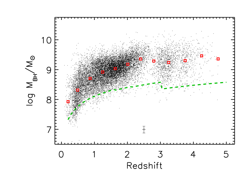
Figure 1.— Redshift distribution of the black hole masses of our quasar sample selected from SDSS DR3. Of the 15,343 quasars detected in the selected sky area at $z\geq 0.2$, mass estimates were possible for 14,584 quasars. Of these, 14,434 quasars have redshifts between 0.3 and 5.0. The median mass in each redshift bin shown in Figure 2 is marked with the (red) open box. The median propagated black hole mass measurement error is shown in the lower part of the diagram. For reference, the (green) dashed curve indicates the faint SDSS flux limits folded with a line width of 2000 km s^-1.

3. Black Hole Mass Estimates

The specific mass scaling relations we use are equations 5 and 7 of Vestergaard & Peterson (2006) based on the FWHM of H$\beta$ and C iv and a new relationship for the Mg ii emission line based on high-quality data from the SDSS DR3 quasar sample (M. Vestergaard et al., in preparation). For each quasar a black hole mass estimate is computed for each of the H$\beta$, Mg ii, and C iv emission lines rendered suitable for mass estimates (§ 2). The final black hole mass was computed as the variance weighted average of the individual mass estimates. The mass estimates based on the individual emission lines match well within their errors.

Figure 1 shows the redshift distribution of the black hole masses. Its detailed shape is mainly a consequence of the survey properties and limitations: (a) the scarcity of quasars at 2.2 $\leq z\leq$ 3.0 is due to inefficient quasar selection, discussed later and (b) the lower boundary is determined mainly by the faint survey flux limits ($i<$ 19.1 mag at $z<$ 3.0; $i<$ 20.2 mag at $z\geq 3$). While the bright flux limit ($i>$ 15 mag) of SDSS is expected to eliminate the most massive black holes at $z<$ 1, this does not have a strong impact on the current study. Judging from the comparison made (Jester et al. 2005) between the Bright Quasar Survey (hereafter BQS, Schmidt and Green 1983) and SDSS the surface density of quasars brighter than $i$ = 15.0 is such that at least 6 such bright quasars are expected in the 1622 square degrees of the current sample; this is a lower limit since the BQS itself is incomplete. If these bright quasars follow the same redshift distribution as the BQS quasars detected by SDSS, they will mostly lie at $z\stackrel{{\scriptstyle\scriptscriptstyle<}}{{\scriptstyle{}_{\sim}}}$ 0.25, below the minimum redshift bound (0.3) of the mass functions. Also, no upper limit in line width is imposed that would place an upper bound on the black hole masses. While we do deselect low quality emission line profiles (see § 2) this process applies to all profile widths (and thus all black hole masses). Given our large sample size (nearly 15,000 quasars) and that we know of no selection effects that would systematically deselect the most massive black holes, it is fair to conclude that the upper bound in black hole mass is real. The mass distribution in Figure 1 therefore confirms with larger numbers the results from previous studies (e.g., Corbett et al. 2003; Warner et al. 2003; Netzer 2003; McLure & Dunlop 2004; Vestergaard 2004; Kollmeier et al. 2006; Netzer & Trakhtenbroot 2007; see also Vestergaard 2006, 2007; Shen et al. 2007) that find the detected quasars at high redshift have black hole masses between a few times 10⁸$M_{\odot}$ to 10¹⁰$M_{\odot}$ with typical mass of order 10⁹ $M_{\odot}$.

4. Black Hole Mass Functions

The differential quasar black hole mass function, $\Psi$($M_{\rm BH}$,$z$) is the space density of quasar black holes (i.e., the number of black holes per unit comoving volume) per unit black hole mass as a function of black hole mass and redshift. We calculate this space density in different mass and redshift bins using the 1/$V_{a}$ method following Warren, Hewett, and Osmer (1994), where $V_{a}$ is the accessible volume, defined by Avni and Bahcall (1980). We adopt the method of Fan et al. (2001) of including the selection function of the quasars: we interpolate the selection function between the grid points defined by the quasar luminosity and redshift and integrate over the selection function in determining $V_{a}$; see equation (6) of Fan et al. The SDSS DR3 quasar selection function for our quasar sample is published by R06. The mass function (and its statistical uncertainty) is given by

$$\Psi(<\!M\!>,<\!z\!>)=\sum_{i}\frac{1}{V_{a,i}\;\Delta M_{\rm BH}},$$ (1a)

$$\sigma(\Psi)=\left[\sum_{i}\left(\frac{1}{V_{a,i}\;\Delta M_{\rm BH}}\right)^{2}\right]^{1/2},$$ (1b)

where $<\!M\!>$ and $<\!z\!>$ are the average mass and redshift of each mass bin of size $\Delta M_{\rm BH}$ and redshift bin of size $\Delta z$ and index $i$ refers to each individual quasar in this mass and redshift bin. In Figure 2 we show the mass functions at a range of redshifts. For better comparison, the redshift bins are chosen to be those used for the luminosity function for this sample (R06). The data points with large errors are typically due to very few quasars residing in those mass bins.

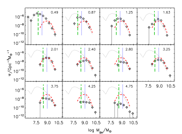
Figure 2.— Mass functions of active supermassive black holes in the quasar sample at a range of redshifts (open diamonds; error bars denote the Poisson statistical uncertainty). The mean redshift of each redshift bin is labeled. The boundaries of the redshift bins are: 0.3, 0.68, 1.06, 1.44, 1.82, 2.2, 2.6, 3.0, 3.5, 4.0, 4.5, 5.0. In each panel the $z$ = 0.49 and 2.01 mass functions are also shown as (black) dotted and (red) dashed curves for reference. The vertical (green) dashed and (blue) dotted lines mark the masses of two fiducial black holes at the mean redshift of the z-bin, emitting a luminosity equal to the survey flux limit, and around which the broad emission line gas is moving at 2000 km s^-1 and 3500 km s^-1 (FWHM), respectively. Incompleteness is expected for black hole masses below the 2000 km s^-1 equivalent fiducial mass value, but may also affect bins of higher mass values. See text for details and discussion.

5. Discussion and Summary

For each redshift bin in Figure 2 the mass function displays a rise and fall in the mass distribution. The decline toward higher masses is expected to be intrinsic to the quasar population (§ 3); while the uncertainty in the mass estimates will affect the accuracy of the slope value, it is too small to be responsible for the decline. We determine a typical high-end slope $\beta$ of about $-$3.3 ($\Psi\propto M^{\beta}$) with uncertainties between 0.4 to 1.3 for the mass functions below a redshift of 4. At the mean redshifts of 4.25 and 4.75 the high-end slope ‘flattens’ to $\beta\approx-2.9\pm 1.1$ and $\beta\approx-1.9\pm 1.7$, respectively. The mass function at redshift 4.75 is based on very few black holes at each mass bin, especially for $M_{\rm BH}$ $\geq 10^{10}$$M_{\odot}$, so the shape is somewhat uncertain. The mass functions are clearly consistent with a constant slope across all epochs. This is also easily verified in Figure 2 by the reference curves for the mass functions at $z$=0.49 (black dotted) and at $z$= 2.01 (red dashed) which also show the space density of high mass black holes slightly increases at $z\stackrel{{\scriptstyle\scriptscriptstyle>}}{{\scriptstyle{}_{\sim}}}$ 1.

The slope of the mass functions is consistent with the bright end slope of the quasar luminosity function ($\beta\approx-3.3$; Croom et al. 2004; R06) to within the uncertainties with the exception that the latter flattens above a redshift of 4 (to $\beta=-2.5$; Schmidt et al. 1995; Fan et al. 2001). Another difference is the relative normalizations. The mass functions exhibit a change in space density for a given mass of only a factor of a few between $z$ = 0.5 and $z$ = 2 (cf. the dotted and dashed curves in Fig 2), while the space density of quasars brighter than $\sim$ $-$27 mag drops 2 orders of magnitude or more between redshifts 2 and 0.5 (Fig. 18, R06). While there is no one-to-one correspondence between a given mass value and a given luminosity value since black holes radiate at a range of (Eddington) rates, the different space density changes show that the cumulative volume density of $L/M$ ($\propto L/L_{\rm Edd}$) decreases toward low redshift. This confirms what we already know based on the declining space density of active nuclei at later epochs (e.g., R06): low redshift black holes are typically less active.

In Figure 2, a characteristic peak shift to higher mass values with redshift is seen. It is important to establish the reality of these peaks and their shifts, since this would have intriguing cosmological implications. For one, it would be a clear manifestation of cosmic down-sizing: the most massive black holes were more actively accreting early in the universe and with time progressively less massive black holes dominate the population of actively accreting black holes. Alternatively, the down-turn toward lower mass values may simply be due to incompleteness of the sample, as the source selection is based on the source luminosity and broad-band colors, not on black hole mass. As a result, we will not obtain a sharp lower boundary in mass (as we do in the luminosity distribution) but a decrease in space density below the survey flux limits, owing to the distribution of black hole masses at a given luminosity. Unfortunately, the SDSS does not go deep enough for us to make meaningful cuts in black hole mass for the current sample, as will be clear later.

The best way to assess which part of the down-turn is intrinsic requires detailed simulations that include the uncertainties in the mass estimates, the selection function, and the flux limits. Since this is non-trivial we will address this in a forthcoming paper (B. Kelly et al., in preparation). Here, we instead perform crude checks as follows. Firstly, in Figure 2 we mark the masses of a fiducial source at the mean bin redshift with a continuum luminosity equivalent to the flux limit at that redshift and a broad line width of 2000 km s^-1 (green dashed vertical line) and 3500 km s^-1 (blue dotted vertical line), respectively; 2000 km s^-1 is the canonical lower line width for which a source is a bona-fide quasar and 3500 km s^-1 is the median linewidth for nearby quasars. There are objects below the (green) dashed line since the observed $i$-band magnitude contains emission contribution in addition to the power-law continuum luminosity used for the mass estimates (see § 2). Nonetheless, these fiducial masses do yield a guideline location of the SDSS flux limits in the mass parameter space, and their location close to the peak of the mass distribution suggests that the peak shift is simply due to the survey flux limits.

Given the non-trivial relationship between the $i$-band magnitude and the monochromatic luminosity, we also performed a simple simulation with the aim of minimizing selection effects. We generated a mock catalog of quasars covering redshifts between 0.2 to 5.0 and bolometric luminosities between $10^{42}$ erg s^-1 and $10^{48}$ erg s^-1. For each ($L,z$) grid point we computed the distribution of black hole masses by applying the typical observed line width distribution for these $L$ and $z$ values. The mass functions based on this mock catalog (not shown) do not display the narrowly peaked distributions seen in Figure 2, but display a slower continued rise in the distribution below the high mass fast decline and a sharp downturn at the lowest masses which coincides with the lower luminosity bound. No downturn is seen at the low mass end if a sharp cut in black hole mass is imposed. Hence, this mock catalog confirms the earlier indication that the low-mass downturn in the observed mass functions is a consequence of the relatively narrow luminosity range probed by SDSS broadened by the line width distribution, especially at higher redshift. We thus conclude that the peaks and their shifts with redshift are mainly due to incompleteness of active black holes near the survey flux limits. These crude checks are, however, unable to verify which part of the turnover is trustworthy. The mass functions in the lower redshift bins display a slower turnover, part of which may well be real. B. Kelly et al., (in preparation) will present more advanced simulations that address these and related issues.

The space density decline at $z$ $\approx$ 2.8 relative to $z$ = 2.4 and $z$ = 3.25 in Figure 2 is caused by a much lower selection efficiency (by a factor of 8; Fig. 6 of R06) as quasars at these epochs coincide with the stellar loci in the selected color-spaces. This suggests that the completeness level is slightly overestimated at these epochs. This situation is unfortunate since the space density of quasars is known to peak between redshifts of 2 and 3 (e.g., Osmer 1982; Warren et al. 1994; Schmidt, Schneider, & Gunn 1995; Fan et al. 2001). It is thus not possible with the current sample to get a complete picture of how the space density distribution of black holes behave during this important epoch. The Large Bright Quasar Survey (hereafter LBQS; Hewett et al. 1995) of about 1000 quasars, extending to a redshift of 3, offers an opportunity to address these issues further, since this sample is not selected based on broad-band color. The LBQS quasar mass function will be presented by Vestergaard & Osmer (in preparation) and discussed in concert with the DR3 mass function by M. Vestergaard et al. (in preparation), where the mass functions will also be compared to previous work.

References

- Avni & Bahcall (1980) Avni, Y., & Bahcall, J. N. 1980, ApJ, 235, 694
- (2) Bruzual, X. & Charlot, X. 2003, MNRAS, 344, 1000
- Cattaneo et al. (2006) Cattaneo, A., Dekel, A., Devriendt, J., Guiderdoni, B., & Blaizot, J. 2006, MNRAS, 370, 1651
- (4) Corbett, E.A., et al. 2003, MNRAS, 343, 705
- Croom et al. (2004) Croom, S. M., Smith, R. J., Boyle, B.J., Shanks, T., Miller, L., Outram, P.J., and Loaring, N. S., 2004, MNRAS, 349, 1397
- (6) Fan, X. et al. 2001, AJ, 121, 54
- Ferrarese and Merritt (2000) Ferrarese, L. & Merritt, D. 2000, ApJ, 539, L9
- (8) Gebhardt, K. et al. 2000a, ApJ, 539, L13
- (9) Gebhardt, K. et al. 2000b, ApJ, 543, L5
- Genzel et al. (2003) Genzel, R., et al. 2003, ApJ, 594, 812
- Ghez et al. (2005) Ghez, A. M., Salim, S., Hornstein, S. D., Tanner, A., Lu, J. R., Morris, M., Becklin, E. E., & Duchêne, G. 2005, ApJ, 620, 744
- Granato et al. (2004) Granato, G. L., De Zotti, G., Silva, L., Bressan, A., & Danese, L. 2004, ApJ, 600, 580
- Harms et al. (1994) Harms, R. J., et al. 1994, ApJ, 435, L35
- (14) Hewett, P. C., Foltz, C. B., & Chaffee, F.H. 1995, AJ, 109, 1498
- Jester et al. (2005) Jester, S., et al. 2005, AJ, 130, 873
- Kang et al. (2006) Kang, X., Jing, Y. P., & Silk, J. 2006, ApJ, 648, 820
- Kollmeier et al. (2006) Kollmeier, J. A., et al. 2006, ApJ, 648, 128
- Magorrian et al. (1998) Magorrian, J. et al. 1998, AJ, 115, 2285
- (19) Mclure, R. & Dunlop, J. 2004, MNRAS, 352, 1390
- Netzer (2003) Netzer, H. 2003, ApJ, 583, L5
- (21) Netzer, H. & Traktenbroot, B. 2007, ApJ, 654,754
- Onken et al. (2004) Onken, C.A., et al. 2004, ApJ, 615, 645
- Osmer (1982) Osmer, P. S. 1982, ApJ, 253, 28
- Peterson et al. (2004) Peterson, B.M. et al. 2004, ApJ, 613, 682
- Richards et al. (2006) Richards, G. T., et al. 2006, AJ, 131, 2766 (R06)
- Salpeter (1964) Salpeter, E. E. 1964, ApJ, 140, 796
- Schlegel et al. (1998) Schlegel, D. J., Finkbeiner, D. P., & Davis, M. 1998, ApJ, 500, 525
- Schneider et al. (2005) Schneider, D. et al. 2005, AJ, 130, 367
- Schmidt & Green (1983) Schmidt, M., & Green, R. F. 1983, ApJ, 269, 352
- Schmidt, Schneider, & Gunn (1995) Schmidt, M., Schneider, D. P., & Gunn, J. E. 1995, AJ, 110, 68
- (31) Shen, Y., Greene, J. E., Strauss, M., Richards, G. T., Schneider, D.P. 2007, preprint (arXiv:0709.3098v1)
- Springel et al. (2005) Springel, V., Di Matteo, T., & Hernquist, L. 2005, ApJ, 620, L79
- Trump et al. (2006) Trump, J. R., et al. 2006, ApJS, 165, 1
- Véron-Cetty et al. (2004) Véron-Cetty, M.-P., Joly, M., & Véron, P. 2004, A&A, 417, 515
- Vestergaard (2002) Vestergaard, M. 2002, ApJ, 571, 733
- Vestergaard (2004) Vestergaard, M. 2004, ApJ, 601, 676
- Vestergaard (2006) Vestergaard, M. 2006, New Astronomy Review, 50, 817
- Vestergaard (2007) Vestergaard, M. 2007, in the STScI Spring Symposium 2007 on ’Black Holes’, ed. A. Koekemoer, Cambridge University Press, in press
- Vestergaard & Peterson (2006) Vestergaard, M., & Peterson, B. M. 2006, ApJ, 641, 689
- Vestergaard & Wilkes (2001) Vestergaard, M., & Wilkes, B. J. 2001, ApJS, 134, 1
- Warner et al. (2003) Warner, C., Hamann, F., & Dietrich, M. 2003, ApJ, 596, 72
- Warren et al. (1994) Warren, S. J., Hewett, P. C., & Osmer, P. S. 1994, ApJ, 421, 412
- Wyithe & Padmanabhan (2006) Wyithe, J. S. B., & Padmanabhan, T. 2006, MNRAS, 372, 1681
- (44) Zeldovich, Y. B. & Novikov, I. 1964, Sov. Phys. Dokl. 158, 811