Quantum gravitational corrections to the stress-energy
tensor around the rotating BTZ black hole

Abstract

Modes emerging out of a collapsing black hole are red-shifted to such an extent that Hawking radiation at future null infinity consists of modes that have energies beyond the Planck scale at past null infinity. This indicates that physics at the Planck scale may modify the spectrum of Hawking radiation and the associated stress-energy tensor of the quantum field. Recently, it has been shown that, the T-duality symmetry of string fluctuations along compact extra dimensions leads to a modification of the standard propagator of point particles in quantum field theory. At low energies (when compared to the string scale), the modified propagator is found to behave as though the spacetime possesses a minimal length, say, $L_{{}_{\rm P}}$, which we shall assume to be of the order of the Planck length. We utilize the duality approach to evaluate the modified propagator around the rotating Banados-Teitelboim-Zanelli black hole and show that the propagator is finite in the coincident limit. We compute the stress-energy tensor associated with the modified Green’s function and illustrate graphically that the quantum gravitational corrections turn out to be negligibly small. We conclude by briefly commenting on the results we have obtained.

I Why do we need to consider Planck scale physics?

Hawking radiation primarily arises due to the asymmetry in the extent of the redshift and the blueshift of the modes of a quantum field as they propagate through matter that is collapsing gravitationally and, eventually, goes on to become a black hole hawking-op . Consider a typical mode that constitutes Hawking radiation at the future null infinity (i.e. at ${\cal I}^{+}$), say, the mode where the intensity of the radiation is the maximum and whose wavelength can be identified, for instance, using Wein’s law. When one traces such a mode back to the past null infinity (i.e. to ${\cal I}^{-}$) where the initial conditions are imposed on the quantum field, one finds that the energy of the mode turns out to be way beyond the Planck scale. (This feature seems to have been originally noticed in Ref. wald-1976 ; in this context, also see Ref. wald-1984 .) As Hawking radiation mostly consists of modes that leave the future event horizon just before its formation, such a phenomenon essentially occurs due to the enormous red-shifting of the modes near the horizon. This behavior then raises the question as to whether the Planck scale effects will modify the spectrum of Hawking radiation and the associated stress-energy tensor of the quantum field.

There has been a sufficient amount of effort in the literature towards understanding the effects of Planck scale physics on Hawking radiation (for the earliest discussions, see Refs. jacobson-1993-99 ; brout-1995-99 ; hambli-1996 ; parentani-1999-2001 , and, for relatively recent efforts, see Refs. casadio-2006 ; agullo-2007 ). In the absence of a workable quantum theory of gravity, to study the Planck scale effects, most of these efforts (apart from one notable exception, see Ref. hambli-1996 ) consider phenomenological models constructed by hand—models which purportedly contain one or more features of the actual effective theory obtained by integrating out the gravitational degrees of freedom. These models either introduce new features in the standard dispersion relation jacobson-1993-99 ; brout-1995-99 , or work with a classical fluctuating geometry parentani-1999-2001 , or assume that the spacetime coordinates are non-commutative casadio-2006 . Often—though, we should hasten to add—but, not always, these high energy models do not preserve local Lorentz invariance. Moreover, some of them either consider a simpler model of Hawking radiation (say, the popular model of a moving mirror in flat space-time casadio-2006 ) rather than the actual situation, or just consider the spherically symmetric (i.e. the $\ell=0$) mode in higher dimensional cases, which, essentially, reduces to studying the effects in $(1+1)$-dimensions. Our aim in this work, is to use a locally Lorentz invariant approach to evaluate the Planck scale modifications to stress-energy tensor around a black hole without resorting to such approximations.

General arguments based on the merging of essential concepts from general relativity and quantum mechanics seem to indicate that it may not be possible to probe spacetime intervals smaller than the Planck length, say, $L_{{}_{\rm P}}$ (see, for example, Ref. paddy-1987 ). An approach that introduces such a ‘zero-point length’ into standard quantum field theory while preserving local Lorentz invariance is the so-called principle of path integral duality (for the original discussion, see Refs. paddy-1997-98 ; for various applications of the approach, see Refs. srini-1998 ; shanki-2001 ; sriram-2006 ). Interestingly, it has been shown that, at low energies (when compared to the string scale), the modified propagator of matter fields obtained through such an approach is equivalent to taking into account the string fluctuations propagating along compact extra dimensions smailagic-2003 ; spallucci-2005 ; fontanini-2006 . Effectively, the path integral duality approach can be said to provide a prescription to evaluate the modified Green’s function of a free quantum field that is propagating in a given classical background (for further details, see the following section). In this work, we shall use this prescription to evaluate the modified Green’s function and the Planck scale corrections to the stress-energy tensor around a specific black hole.

In $(3+1)$-dimensions, it proves to be difficult to evaluate the two-point function exactly around even the simplest of black holes. As a result, the stress-energy tensor of a quantum field around, say, the Schwarzschild black hole has been evaluated only under an approximation (see, for example, Refs. page-1982 ; campos-1998 ; phillips-2003 ). In contrast, the spacetime around the $(2+1)$-dimensional, rotating Banados-Teitelboim-Zanelli (BTZ, hereafter) black hole banados-1992-93 ; carlip-1995 ; carlip-1998 provides a situation wherein it is possible to calculate the two-point function in a closed form steif-1994 ; lifschytz-1994 ; shiraishi-1994 ; ichinose-1995 ; mann-1997 ; bystenko-1998 ; binosi-1999 . We shall utilize this feature to compute the duality modified propagator and the corresponding Planck scale corrections to the standard stress-energy tensor around the rotating BTZ black hole.

The remainder of this paper is organized as follows. In the following section, we shall briefly outline as to how the principle of path integral duality modifies the two-point function of a free quantum field evolving in a given spacetime. In Section III, we evaluate the modified propagator around the rotating BTZ black hole, and show that the path integral duality approach regulates the ultra-violet behavior of the two-point function. In Section IV, we evaluate the stress-energy tensor associated with the modified two-point function and graphically illustrate the form of the Planck scale modifications to the stress-energy tensor. Finally, in Section V, we close with a brief discussion on the results we have obtained.

Before we proceed, a few words on our notations and conventions are in order. We shall work in $(2+1)$-dimensions and adopt the metric signature of $(-,+,+)$. Also, for convenience, we shall denote the set of three coordinates $x^{\mu}$ as ${\tilde{x}}$, and use natural units such that $G=\hbar=c=1$.

II String fluctuations, duality and the modified Green’s function

Recently, it was shown that, when the fluctuations of closed strings along compact extra dimensions are taken into account, one arrives at an effective propagator for point particles that is regular at high energies fontanini-2006 . It was found that, the $T$-duality symmetry between the topologically non-trivial excitations and the winding modes of the strings around the compact dimensions leads to a modified propagator in the Minkowski vacuum wherein the original spacetime interval $({\tilde{x}}-{\tilde{x}}^{\prime})^{2}$ between the two spacetime events ${\tilde{x}}$ and ${\tilde{x}}^{\prime}$ is replaced by $[({\tilde{x}}-{\tilde{x}}^{\prime})^{2}+L_{{}_{\rm P}}^{2}]$, where, as we mentioned above, $L_{{}_{\rm P}}$ denotes the Planck length. Thus, effectively, the string fluctuations introduce a zero point length $L_{{}_{\rm P}}$ into the standard field theory.

A similar modification of the Minkowski propagator has been obtained earlier by invoking the principle of path integral duality paddy-1997-98 . Recall that, in standard quantum field theory, the path integral amplitude for a path connecting events ${\tilde{x}}$ and ${\tilde{x}^{\prime}}$ in a given spacetime is proportional to the proper length, say, ${\cal R}({\tilde{x}},{\tilde{x}^{\prime}})$, between the two events. The duality principle proposes that the path integral amplitude should be invariant under the transformation ${\cal R}\rightarrow\left(L_{{}_{\rm P}}^{2}/{\cal R}\right)$. Operationally, it turns out to be convenient to express the effect of the duality approach and the string fluctuations on the propagator in terms of the Schwinger’s proper time formulation paddy-1997-98 . One finds that, in such a formulation, the string fluctuations and the duality approach effectively modify the weightage given to a point particle of mass $m$, from $\exp\;-(i\,m^{2}\,s)$ to $\exp\;-[i\,(m^{2}\,s-(L_{{}_{\rm P}}^{2}/4\,s))]$.

Consider a free scalar field of mass $m$ that is propagating in a given classical gravitational background described by the metric tensor $g_{\mu\nu}$. Let us further assume that the field is non-minimally coupled to gravity. In Schwinger’s proper time formalism, the two-point function corresponding to such a scalar field can be expressed as schwinger-1951 ; dewitt-1975

$$G({\tilde{x}},{\tilde{x}^{\prime}})=i\,\int\limits_{0}^{\infty}ds\;K({\tilde{x}},{\tilde{x}^{\prime}};s),$$ (1)

where $K({\tilde{x}},{\tilde{x}^{\prime}};s)$ is defined as

$$K({\tilde{x}},{\tilde{x}^{\prime}};s)\equiv\langle{\tilde{x}}|\,e^{i\,\left({\widehat{\Box}}-m^{2}-\xi\,R\right)\,s}\,|{\tilde{x}^{\prime}}\rangle,$$ (2)

and $R$ is the curvature of the background spacetime with $\xi$ being the coefficient of the non-minimal coupling. In other words, the quantity $K({\tilde{x}},{\tilde{x}^{\prime}};s)$ is the path integral amplitude for a quantum mechanical system described by the following Hamiltonian:

$${\widehat{H}}=-\left({\widehat{\Box}}-m^{2}-\xi\,R\right)\equiv-\frac{1}{\sqrt{-g}}\,\partial_{\mu}\left(\sqrt{-g}\,g^{\mu\nu}\,\partial_{\nu}\right)+m^{2}+\xi\,R.$$ (3)

As we mentioned, the effects due to path integral duality or, equivalently, the string fluctuations, correspond to modifying the expression (1) above for the two-point function to paddy-1997-98 ; fontanini-2006

$$G^{\rm M}({\tilde{x}},{\tilde{x}^{\prime}})=i\,\int\limits_{0}^{\infty}ds\;\,e^{iL_{{}_{\rm P}}^{2}/4\,s}\;\,K({\tilde{x}},{\tilde{x}^{\prime}};s).$$ (4)

In the following section, we shall make use of this prescription to evaluate the modified two-point function around the rotating BTZ black hole.

III The modified Green’s function around the rotating BTZ black hole

The rotating BTZ black hole is an axially symmetric vacuum solution of the Einstein’s equations in three-dimensional anti-de Sitter spacetime (AdS₃, hereafter). It can be conveniently represented as AdS₃ identified under a discrete subgroup of its isometry group banados-1992-93 ; carlip-1995 ; carlip-1998 .

Recall that AdS₃ is a maximally symmetric space sourced by a negative cosmological constant, say, $-\ell^{-2}$. AdS₃ can be described by the line-element

$$ds^{2}=-\left(\frac{{\hat{r}}^{2}}{\ell^{2}}-1\right)\,d{\hat{t}}^{2}+\left(\frac{{\hat{r}}^{2}}{\ell^{2}}-1\right)^{-1}\,d{\hat{r}}^{2}+{\hat{r}}^{2}\,d{\hat{\phi}}^{2},$$ (5)

where $-\infty<({\hat{t}},{\hat{\phi}})<\infty$ and $0<{\hat{r}}<\infty$. It is important to note that the coordinate ${\hat{\phi}}$ in the above line-element has an infinite range and, hence, is not periodic. The rotating BTZ black hole of mass $M$ and angular momentum $J$ can be obtained from the above AdS₃ line-element by making the coordinates ${\hat{t}}$ and ${\hat{\phi}}$ suitably periodic as follows banados-1992-93 ; carlip-1995 ; carlip-1998 :

$$({\hat{t}},{\hat{r}},{\hat{\phi}})\equiv\left[({\hat{t}}-2\,\pi\,n\,\ell\,\alpha_{{}_{-}}),{\hat{r}},({\hat{\phi}}+2\,\pi\,n\,\alpha_{{}_{+}})\right],$$ (6)

where, $n$ is an integer, and the quantities $\alpha_{\pm}$ are given by

$$\alpha_{{}_{\pm}}=\left(\frac{1}{2}\right)\,\left[\sqrt{M+(J/\ell)}\pm\sqrt{M-(J/\ell)}\right].$$ (7)

On redefining the coordinates $({\hat{t}},{\hat{r}},{\hat{\phi}})$ as follows (see, for instance, Ref. steif-1994 ):

$${\hat{t}}=\left(\alpha_{{}_{+}}\,t-\alpha_{{}_{-}}\,\ell\,\phi\right),\quad{\hat{\phi}}=\left[\alpha_{{}_{+}}\,\phi-(\alpha_{{}_{-}}\,t/\ell)\right],\quad{\rm and}\quad{\hat{r}^{2}}=\left(\frac{r^{2}-(\alpha_{{}_{-}}\,\ell)^{2}}{\alpha_{{}_{+}}^{2}-\alpha_{{}_{-}}^{2}}\right),$$ (8)

we obtain the metric around the rotating BTZ black hole to be banados-1992-93 ; carlip-1995 ; carlip-1998

$$ds^{2}=-\left(\frac{r^{2}}{\ell^{2}}-M\right)\,dt^{2}-J\,dt\,d\phi+\left(\frac{r^{2}}{\ell^{2}}-M+\frac{J^{2}}{4\,r^{2}}\right)^{-1}\,dr^{2}+r^{2}\,d\phi^{2}$$ (9)

with $-\infty<t<\infty$ and $0<r<\infty$. Using the relations (8), it is easy to show that, under the periodicity conditions (6), while $t\to t$, $\phi\to(\phi+2\,\pi\,n)$. Evidently, $\phi$ is a genuine angular coordinate that can be restricted to the domain $0<\phi\leq 2\pi$. The rotating BTZ black hole solution (9) contains two horizons, and the locations of the outer ($r_{{}_{+}}$) and inner ($r_{{}_{-}}$) horizons are given by

$$r_{{}_{\pm}}=\left(\alpha_{{}_{\pm}}\,\ell\right)=\left(\frac{\ell}{2}\right)\,\left[\sqrt{M+(J/\ell)}\pm\sqrt{M-(J/\ell)}\right].$$ (10)

Note that, when $J=0$, $r_{{}_{-}}$ vanishes, and $r_{{}_{+}}=(\sqrt{M}\,\ell)$.

It is clear from the above discussion that, if we can evaluate the Green’s function, say, $G_{{}_{\rm AdS}}({\tilde{x}},{\tilde{x}}^{\prime})$, in AdS₃, then the Green’s function, say, $G_{{}_{\rm BTZ}}({\tilde{x}},{\tilde{x}}^{\prime})$ around the rotating BTZ black hole can be obtained on imposing by hand the periodicity condition (6), and transforming to the black hole coordinates using the relations (8) steif-1994 ; lifschytz-1994 ; shiraishi-1994 ; ichinose-1995 ; mann-1997 ; bystenko-1998 ; binosi-1999 . Therefore, we need to first evaluate the Green’s function in AdS₃. We shall do so by evaluating the quantum mechanical kernel $K({\tilde{x}},{\tilde{x}}^{\prime};s)$ and using the Schwinger’s proper time expression (1) to arrive at the Green’s function.

In order to calculate the kernel $K({\tilde{x}},{\tilde{x}}^{\prime};s)$ in AdS₃, it turns out to be more convenient to work with the following set of coordinates carlip-1995 :

$$x_{2} = {\hat{r}}^{-1}\;\sqrt{\left({\hat{r}}^{2}-\ell^{2}\right)}\;\,e^{\phi}\;{\rm sinh}\,({\hat{t}}/\ell),$$

$$y = \left(\ell/{\hat{r}}\right)\;e^{\phi},$$ (11)

$$x_{1} = {\hat{r}}^{-1}\;\sqrt{\left({\hat{r}}^{2}-\ell^{2}\right)}\;\,e^{\phi}\;{\rm cosh}\,({\hat{t}}/\ell).$$

In terms of these new coordinates, the AdS₃ line-element (5) reduces to

$$ds^{2}=(\ell^{2}/y^{2})\,\left(-dx_{2}^{2}+dy^{2}+dx_{1}^{2}\right),$$ (12)

which, evidently, is conformal to flat spacetime. The kernel of a massive and non-minimally coupled scalar field propagating in the above conformally flat line-element can be easily evaluated using the method of spectral decomposition (see, for instance, the Appendix in Ref. binosi-1999 ). We find that the kernel can be expressed as mann-1997 ; bystenko-1998 ; binosi-1999

$$K({\tilde{x}},{\tilde{x}}^{\prime};s)=\left(\frac{1}{(4\pi\,i\,s)^{3/2}}\right)\;\left(\frac{\sigma({\tilde{x}},{\tilde{x}}^{\prime})/\ell}{\sinh\left[\sigma({\tilde{x}},{\tilde{x}}^{\prime})/\ell\right]}\right)\;\exp\,\left[i\,(\sigma^{2}({\tilde{x}},{\tilde{x}}^{\prime})/4\,s)-i\,(b\,s/\ell^{2})\right],$$ (13)

where $b=\left[1+(m\,\ell)^{2}+\xi\,R\,\ell^{2}\right]$, with $R=-(6/\ell^{2})$ being the Ricci scalar (a constant in AdS₃). The quantity $\sigma({\tilde{x}},{\tilde{x}}^{\prime})$ denotes the geodesic distance between the two points ${\tilde{x}}$ and ${\tilde{x}}^{\prime}$ in AdS₃ and is given by

$${\rm sinh}\,\left[\sigma({\tilde{x}},{\tilde{x}}^{\prime})/2\,\ell\right]=\left[\left(-\left(x_{2}-x_{2}^{\prime}\right)^{2}+\left(y-y^{\prime}\right)^{2}+\left(x_{1}-x_{1}^{\prime}\right)^{2}\right)/4\,y\,y^{\prime}\right]^{1/2}.$$ (14)

(It may be useful to note that the geodesic distance in AdS₃, viz. $\sigma({\tilde{x}},{\tilde{x}}^{\prime})$, can be conveniently expressed in terms of the chordal distance between the two points in the embedding space.) In terms of the original coordinates $({\hat{t}},{\hat{r}},{\hat{\phi}})$, the quantity $\sigma({\tilde{x}},{\tilde{x}}^{\prime})$ turns out to be

$$\!\!\!\!\!\!\!\!\!\!\!\!\!\!\!\!{\rm sinh}\left[\sigma({\tilde{x}},{\tilde{x}}^{\prime})/2\ell\right]$$

$$\;=\left(\sqrt{2}\,\ell\right)^{-1}\biggl{[}-\,\sqrt{\left({\hat{r}}^{2}-\ell^{2}\right)\,\left({\hat{r}}^{\prime 2}-\ell^{2}\right)}\;\;{\rm cosh}\left[\left({\hat{t}}-{\hat{t}}^{\prime}\right)/\ell\right]$$

$$\qquad\qquad\qquad\qquad\qquad\qquad\qquad\qquad-\;\ell^{2}+{\hat{r}}\;{\hat{r}}^{\prime}\;{\rm cosh}\left({\hat{\phi}}-{\hat{\phi}}^{\prime}\right)\biggr{]}^{1/2}.\quad$$ (15)

On using the expression (1), the Green’s function corresponding to the kernel (13) can then be immediately evaluated to be mann-1997 ; bystenko-1998 ; binosi-1999

$$G_{{}_{\rm AdS}}({\tilde{x}},{\tilde{x}}^{\prime})\\ =\left(\frac{1}{4\,\pi\,\ell}\right)\;\left(\frac{1}{\sinh\left[\sigma({\tilde{x}},{\tilde{x}}^{\prime})/\ell\right]}\right)\;\exp{-\left[\sqrt{b}\;\sigma({\tilde{x}},{\tilde{x}}^{\prime})/\ell\right]}.$$

We should mention here that this Green’s function corresponds to a particular choice of boundary condition (actually, the Dirichlet condition mann-1997 ; bystenko-1998 ; binosi-1999 ) that is required to be imposed at spatial infinity in AdS spacetimes (see, for example, Refs. ads ).

The Green’s function around the rotating BTZ black hole can now be obtained by imposing the periodicity condition (6) in the AdS₃ Green’s function (III), and transforming into the black hole coordinates using the relations (8). The BTZ Green’s function can be expressed as steif-1994 ; lifschytz-1994 ; shiraishi-1994 ; ichinose-1995 ; mann-1997 ; bystenko-1998 ; binosi-1999

$$G_{{}_{\rm BTZ}}({\tilde{x}},{\tilde{x}}^{\prime})=\left(\frac{1}{4\,\pi\,\ell}\right)\;\sum\limits_{n=-\infty}^{\infty}\left(\frac{1}{\sinh\left[\sigma_{n}({\tilde{x}},{\tilde{x}}^{\prime})/\ell\right]}\right)\,\exp{-\left[\sqrt{b}\;\sigma_{n}({\tilde{x}},{\tilde{x}}^{\prime})/\ell\right]},$$ (16)

with $\sigma_{n}({\tilde{x}},{\tilde{x}}^{\prime})$ given by

$$\!\!\!\!\!\!\!\!\!\!\!\!\!\!\!\!\!{\rm sinh}\left[\sigma_{n}({\tilde{x}},{\tilde{x}}^{\prime})/2\,\ell\right]$$

$$=\left[2\,\ell^{2}\,\left(\alpha_{{}_{+}}^{2}-\alpha_{{}_{-}}^{2}\right)\right]^{-1/2}\;$$

$$\qquad\quad\times\,\biggl{(}-\,\sqrt{\left[r^{2}-(\alpha_{{}_{+}}\,\ell)^{2}\right]\,\left[r^{\prime 2}-(\alpha_{{}_{+}}\,\ell)^{2}\right]}$$

$$\qquad\qquad\qquad\quad\times\;{\rm cosh}\left[(\alpha_{{}_{+}}/\ell)\;(t-t^{\prime})-\alpha_{{}_{-}}\,(\phi-\phi^{\prime}+2\,\pi\,n)\right]$$

$$\qquad\qquad\quad-\,\left(\alpha_{{}_{+}}^{2}-\alpha_{{}_{-}}^{2}\right)\,\ell^{2}$$

$$\qquad\qquad\quad+\,\sqrt{\left[r^{2}-(\alpha_{{}_{-}}\,\ell)^{2}\right]\,\left[r^{\prime 2}-(\alpha_{{}_{-}}\,\ell)^{2}\right]}$$

$$\qquad\qquad\qquad\quad\times\;{\rm cosh}\left[(\alpha_{{}_{-}}/\ell)\;(t-t^{\prime})-\alpha_{{}_{+}}\,\left(\phi-\phi^{\prime}+2\pi\,n\right)\right]\biggr{)}^{1/2}.$$ (17)

The time translational invariance clearly indicates that the above Green’s function corresponds to the Hawking-Hartle state of the black hole (see, for instance, Ref. birrell-1982 ).

The duality modified Green’s function in AdS₃ can now be obtained by substituting the kernel (13) in the expression (4) and carrying out the integral over $s$. We obtain the duality modified Green’s function in AdS₃ to be

$$\!\!\!\!\!\!\!\!\!\!\!\!\!\!\!\!G_{{}_{\rm AdS}}^{\rm M}({\tilde{x}},{\tilde{x}}^{\prime}) = \left(\frac{1}{4\,\pi\,\ell}\right)\;\left(\frac{\sigma({\tilde{x}},{\tilde{x}}^{\prime})}{\sinh\left[\sigma({\tilde{x}},{\tilde{x}}^{\prime})/\ell\right]}\right)\;\left(\frac{1}{\sqrt{\sigma^{2}({\tilde{x}},{\tilde{x}}^{\prime})+L_{{}_{\rm P}}^{2}}}\right)$$ (18)

$$\qquad\qquad\qquad\qquad\qquad\quad\times\;\exp{-\left(\sqrt{(b/\ell^{2})\;[\sigma^{2}({\tilde{x}},{\tilde{x}}^{\prime})+L_{{}_{\rm P}}^{2}]}\,\right)}$$

with $\sigma({\tilde{x}},{\tilde{x}}^{\prime})$ given by Eq. (15). In the coincidence limit (i.e. when ${\tilde{x}}\to{\tilde{x}}^{\prime}$), $\sigma({\tilde{x}},{\tilde{x}}^{\prime})\rightarrow 0$, and the above modified Green’s function reduces to

$$G_{{}_{\rm AdS}}^{\rm M}({\tilde{x}},{\tilde{x}}^{\prime})=\left(\frac{1}{4\,\pi\,L_{{}_{\rm P}}}\right)\;\exp{-\left(\sqrt{b}\;L_{{}_{\rm P}}/\ell\right)}.$$ (19)

Note that the Green’s function is finite in the coincident limit independent of the nature of the coupling and the mass of the scalar field. This behavior clearly illustrates that the string theory inspired modification regulates the theory at the Planck scale.

The modified Green’s function around the rotating BTZ black hole can be obtained from the above modified Green’s function in AdS₃ as in the standard case. It can be expressed as

$$\!\!\!\!\!\!\!\!\!\!\!\!\!\!\!\!G_{{}_{\rm BTZ}}^{\rm M}({\tilde{x}},{\tilde{x}}^{\prime}) = \left(\frac{1}{4\pi\,\ell}\right)\;\sum\limits_{n=-\infty}^{\infty}\left(\frac{\sigma_{n}({\tilde{x}},{\tilde{x}}^{\prime})}{\sinh\left[\sigma_{n}({\tilde{x}},{\tilde{x}}^{\prime})/\ell\right]}\right)\;\left(\frac{1}{\sqrt{\sigma_{n}^{2}({\tilde{x}},{\tilde{x}}^{\prime})+L_{{}_{\rm P}}^{2}}}\right)$$ (20)

$$\qquad\qquad\qquad\qquad\qquad\;\times\;\exp{-\left(\sqrt{(b/\ell^{2})\;\,[\sigma_{n}^{2}({\tilde{x}},{\tilde{x}}^{\prime})+L_{{}_{\rm P}}^{2}]}\,\right)}$$

with $\sigma_{n}({\tilde{x}},{\tilde{x}}^{\prime})$ given by Eq. (17). The $n\neq 0$ terms are finite in the coincident limit even in the standard (i.e. unmodified) case, while the $n=0$ term corresponds to AdS₃. Obviously, the modified Green’s function around the rotating BTZ black hole is finite in the coincident limit as well.

IV Planck scale modifications to the stress-energy tensor

In this section, we shall first evaluate the standard stress-energy tensor around the rotating BTZ black hole using the two-point function (16). We shall then calculate the Planck scale modifications to the stress-energy tensor using the modified Green’s function (20). For convenience in calculation, we shall restrict ourselves to the case of a massless and conformally coupled scalar field [i.e. when $m=0$, $\xi=(1/8)$ and, hence, $b=(1/4)$]. In such a situation, given the symmetric Green’s function, say, $G({\tilde{x}}_{1},{\tilde{x}}_{2})$, the corresponding mean value of the stress-energy tensor can be expressed as steif-1994 ; lifschytz-1994 ; shiraishi-1994

$$\langle{\hat{T}}_{\mu\nu}\rangle=\lim_{2\to 1}\;{\cal T}_{\mu\nu}^{(1,2)}\;G({\tilde{x}}_{1},{\tilde{x}}_{2}).$$ (21)

The quantity ${\cal T}_{\mu\nu}^{(1,2)}$ is a differential operator and is given by

$${\cal T}_{\mu\nu}^{(1,2)} = \biggl{[}\left({3\over 4}\right)\,\left(\nabla^{1}_{\mu}\,\nabla^{2}_{\nu}\right)-\left({1\over 4}\right)\,g_{\mu\nu}\;g^{\alpha\beta}\,\left(\nabla^{1}_{\alpha}\,\nabla^{2}_{\beta}\right)$$ (22)

$$\qquad\qquad\qquad\quad-\,\left(\frac{1}{4}\right)\,\left(\nabla^{1}_{\mu}\,\nabla^{1}_{\nu}\right)+\left(\frac{R}{96}\right)\,g_{\mu\nu}\biggr{]},$$

where the covariant derivatives $\nabla_{\mu}^{1}$ and $\nabla_{\mu}^{2}$ act on the points ${\tilde{x}}_{1}$ and ${\tilde{x}}_{2}$, respectively, and $R$ denotes the scalar curvature of the background spacetime. It should be mentioned here that the Green’s functions (16) and (20) and, hence, the corresponding stress-energy tensors are valid in the domain $r>r_{{}_{+}}$.

IV.1 The standard (unmodified) stress-energy tensor

Before we proceed to evaluate the Planck scale modifications, let us evaluate the stress-energy tensor in the standard case. Also, let us first consider the simpler situation of the non-rotating BTZ black hole. In such a case, $J=0$, so that $\alpha_{{}_{+}}=M$ and $\alpha_{{}_{-}}=0$. For the case of the Dirichlet boundary condition imposed at spatial infinity, the mean value of the stress-energy tensor associated with a massless and conformally coupled scalar field can be obtained by substituting the Green’s function (16) [with $b=(1/4)$] in the expression (21) above. We find that the resulting stress-energy tensor is diagonal and can be expressed as lifschytz-1994 ; shiraishi-1994

$$\!\!\langle{\hat{T}}^{\mu}_{\nu}\rangle=\left(\frac{M^{3/2}}{32\,\pi\,r^{3}}\right)$$

$$\qquad\qquad\times\;\sum\limits_{n=1}^{\infty}\;\;\left[2+\left(1-\left[1+\left(\frac{M\,\ell^{2}}{r^{2}\,{\rm sinh}^{2}\,(\sqrt{M}\,\pi\,n)}\right)\right]^{-3/2}\right)\;{\rm sinh}^{2}\,(\sqrt{M}\,\pi\,n)\right]$$

$$\qquad\qquad\qquad\qquad\qquad\qquad\qquad\qquad\quad\times\;{\rm sinh}^{-3}\,(\sqrt{M}\,\pi\,n)\;\;{\rm diag.}~{}(1,1,-2)$$

$$\qquad\qquad\qquad\qquad\qquad\quad\;\,+\left(\frac{3\;(r^{2}-M\,\ell^{2})}{r^{2}\;{\rm sinh}^{3}\,(\sqrt{M}\,\pi\,n)}\right)\;\left[1+\left(\frac{M\,\ell^{2}}{r^{2}\;{\rm sinh}^{2}\,(\sqrt{M}\,\pi\,n)}\right)\right]^{5/2}$$

$$\qquad\qquad\qquad\qquad\qquad\qquad\qquad\qquad\quad\times\;{\rm diag.}~{}(1,0,-1).$$ (23)

In order to arrive at this finite result, we have regularized the stress-energy tensor by simply dropping the $n=0$ term which corresponds to the stress-energy tensor in AdS₃. It is well-known that the stress-energy tensor associated with a massless and conformally coupled scalar field vanishes in AdS₃ because of the absence of the trace anomaly in odd dimensions birrell-1982 .

On following the same steps as above, one can, in principle, obtain an analytic expression for the stress-energy tensor around the rotating BTZ black hole (i.e. when $J\neq 0$). The regularization procedure remains the same as in the non-rotating case—one simply drops the $n=0$ term. When the black hole is rotating, one finds that, in addition to the diagonal components, viz. $\langle{\hat{T}}^{t}_{t}\rangle$, $\langle{\hat{T}}^{r}_{r}\rangle$ and $\langle{\hat{T}}^{\phi}_{\phi}\rangle$, the $\langle{\hat{T}}^{t}_{\phi}\rangle$ component turns out to be non-zero as well steif-1994 . While the procedure for calculating the stress-energy tensor is rather straightforward, the resulting expressions turn out to be fairly long to be displayed. Therefore, in order to illustrate the behavior of the stress-energy tensor, in Figures 1 and 2, we have plotted all its components for a couple of different values of the black hole parameters $M$ and $J$.

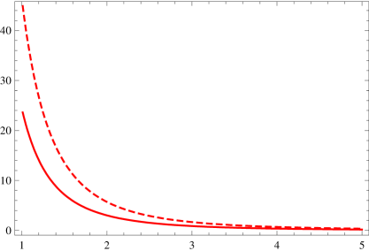
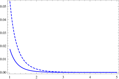
$\ell^{3}\,\langle{\hat{T}}^{t}_{t}\rangle$
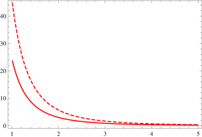
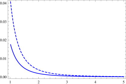
                 $\ell^{3}\,\langle{\hat{T}}^{r}_{r}\rangle$
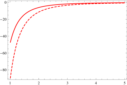
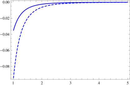
                 $\ell^{3}\,\langle{\hat{T}}^{\phi}_{\phi}\rangle$
              $(r/r_{{}_{+}})$                                                   $(r/r_{{}_{+}})$

Figure 1: The diagonal components of the standard (i.e. the unmodified) stress-energy tensor around the BTZ black hole, viz. $\langle{\hat{T}}^{t}_{t}\rangle$ (on top), $\langle{\hat{T}}^{r}_{r}\rangle$ (in the middle) and $\langle{\hat{T}}^{\phi}_{\phi}\rangle$ (at the bottom), have been plotted as a function of $(r/r_{{}_{+}})$. We have set $\ell=10^{3}$ in all the plots. The red lines (in the left column) and the blue ones (in the right column) correspond to $M=10^{-3}$ and $M=10^{-1}$, respectively. In all these plots, the solid lines correspond to the non-rotating case, while the dashed lines correspond to a rotating black hole with $(J/M\,\ell)=0.95$. We have chosen such an extreme value for $J$ to clearly illustrate the effects due to rotation. It is evident from the above figures that, all the diagonal components of the stress-energy tensor either increase or decrease monotically with the distance from the horizon. Also, qualitatively, rotation does not introduce any new features in these components, but only changes their magnitude. Moreover, the larger the $M$, the smaller is the difference in the magnitude of these components between the non-rotating and rotating cases. Furthermore, this difference is the largest at the horizon, and it decreases with the distance from the horizon of the black hole.

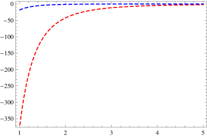
$\ell^{3}\,\langle{\hat{T}}^{t}_{\phi}\rangle$
     $(r/r_{{}_{+}})$

Figure 2: The only non-vanishing, non-diagonal, component of the standard stress-energy tensor, viz. $\langle{\hat{T}}^{t}_{\phi}\rangle$, has been plotted as a function of $(r/r_{{}_{+}})$. Note that this component is zero in the non-rotating case. As in the earlier plots, we have set $\ell=10^{3}$ and chosen $(J/M\,\ell)=0.95$. The red and blue dashed lines again correspond to $M=10^{-3}$ and $M=10^{-1}$, respectively. Evidently, the comments that we had made in the previous figure about the behavior of the diagonal components of the stress-energy tensor apply to this component as well.

Also, to unambiguously demonstrate the effects of rotation, in addition to the non-rotating case, we have plotted the components of the stress-energy tensor for a rotating black hole with an extremely large angular momentum $J$ [we have chosen $(J/M\,\ell)=0.95$] in the two figures. These figures clearly indicate that, rotation only changes the magnitude of the stress-energy tensor and does not alter its qualitative behavior. It either increases or decreases monotonically with the distance from the horizon, as in the non-rotating case. Moreover, the larger the $M$, the smaller is the difference in the stress-energy tensor between the non-rotating and rotating cases. Furthermore, it is evident from the figures that, this difference is the maximum at the horizon and it decreases with the distance from the horizon.

IV.2 Planck scale modifications

The Planck scale modifications to the stress-energy tensor around the rotating BTZ black hole can now be arrived at upon using the modified Green’s function (20) in the expression (21). The structure of the modified stress-energy tensor turns out to be the same as in the standard case. When the black hole is not rotating, the only non-zero components of the modified stress-energy tensor are the diagonal components, which we shall refer to as $\langle{\hat{T}}^{t}_{t}\rangle_{{}_{\rm M}}$, $\langle{\hat{T}}^{r}_{r}\rangle_{{}_{\rm M}}$ and $\langle{\hat{T}}^{\phi}_{\phi}\rangle_{{}_{\rm M}}$. Around a rotating black hole, as in the unmodified case, the only additional non-vanishing component turns out to be $\langle{\hat{T}}^{t}_{\phi}\rangle_{{}_{\rm M}}$. However, as in case of the standard stress-energy tensor around a rotating black hole, the resulting expressions for the modified stress tensor prove to be rather long. We believe that displaying these long and unwieldy expressions may not be necessarily helpful in understanding the Planck scale effects. Therefore, we have again plotted the various components of the modified stress-energy tensor (along with the unmodified ones) in Figures 3 and 4.

In order to distinctly show the Planck scale modifications, in these two figures, we have plotted the non-vanishing components of the stress-energy tensor for an extremely large (and unrealistic) value of $L_{{}_{\rm P}}$ [we have set $(L_{{}_{\rm P}}/r_{{}_{+}})=0.9$]. For convenience in comparison, we have also plotted the corresponding unmodified components in these figures.

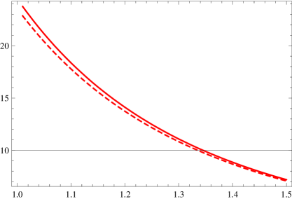
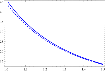
$\ell^{3}\,\langle{\hat{T}}^{t}_{t}\rangle_{{}_{\rm M}}$
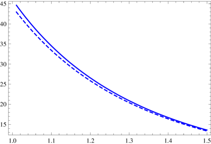
                 $\ell^{3}\,\langle{\hat{T}}^{r}_{r}\rangle_{{}_{\rm M}}$
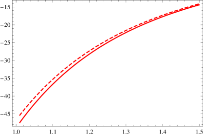
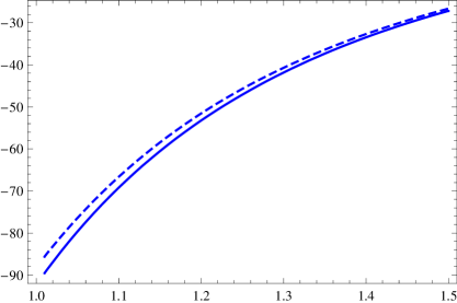
                 $\ell^{3}\,\langle{\hat{T}}^{\phi}_{\phi}\rangle_{{}_{\rm M}}$
              $(r/r_{{}_{+}})$                                                   $(r/r_{{}_{+}})$

Figure 3: The diagonal components of the modified stress-energy tensor around the BTZ black hole, viz. $\langle{\hat{T}}^{t}_{t}\rangle_{{}_{\rm M}}$ (at the top), $\langle{\hat{T}}^{r}_{r}\rangle_{{}_{\rm M}}$ (in the middle) and $\langle{\hat{T}}^{\phi}_{\phi}\rangle_{{}_{\rm M}}$ (at the bottom), have been plotted as a function of $(r/r_{{}_{+}})$. We have also plotted the corresponding standard components for comparison. We have set $\ell=10^{3}$ and $M=10^{-3}$ in all the plots. The red lines (in the left column) and the blue ones (in the right column) correspond to the non-rotating black hole and a rotating one with $(J/M\,\ell)=0.95$, respectively. In all these plots, the solid lines correspond to the standard case wherein $L_{{}_{\rm P}}=0$, while the dashed lines correspond to the modified case with $(L_{{}_{\rm P}}/r_{{}_{+}})=0.9$. We have chosen such an extremely large value of $L_{{}_{\rm P}}$ and have also plotted over a smaller range in $(r/r_{{}_{+}})$ in order to distinctly demonstrate the Planck scale effects. The above figures clearly indicate that the Planck scale effects do not alter the qualitative behavior of the diagonal components of the stress-energy tensor. Note that the Planck scale modifications are the largest at the horizon and these modifications decrease monotonically with the distance from the horizon.

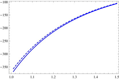
$\ell^{3}\,\langle{\hat{T}}^{t}_{\phi}\rangle_{{}_{\rm M}}$
     $(r/r_{{}_{+}})$

Figure 4: The only non-zero and non-diagonal component of the modified stress-energy tensor, viz. $\langle{\hat{T}}^{t}_{\phi}\rangle_{{}_{\rm M}}$, has been plotted as a function of $(r/r_{{}_{+}})$. As in the standard case, we find that this component vanishes in the modified case when the black hole is not rotating. We have set $\ell=10^{3}$ and chosen $(J/M\,\ell)=0.95$ in these plots. For comparison, we have also plotted the corresponding component in the unmodified case. The blue solid line corresponds to the standard case (i.e. when $L_{{}_{\rm P}}=0$), while the blue dashed line corresponds to the modified case with $(L_{{}_{\rm P}}/r_{{}_{+}})=0.9$. It is evident that the comments that we had made in the previous figure about the behavior of the diagonal components of the modified stress-energy tensor apply to this component as well.

It is evident from the figures that the Planck scale effects (as taken into account through the duality principle) do not modify the stress-energy tensor to any appreciable extent. Nor do they alter its qualitative behavior. As in the standard case, the modified stress-energy tensor either increases or decreases monotonically with distance from the horizon. Moreover, the Planck scale modifications prove to be significant only very close to the horizon. We find that, for an $L_{{}_{\rm P}}$ as large as $(0.9\;r_{{}_{+}})$, the change in the stress-energy tensor is of the order of $3$–$5\%$ at the horizon. For any smaller value of $L_{{}_{\rm P}}$, the modified case turns out to be completely indistinguishable from the unmodified one. Therefore, we can conclude that, for any realistic $L_{{}_{\rm P}}$, the modifications are completely negligible. This result corroborates similar conclusions that have been arrived at earlier in the literature (see, for example, Refs. jacobson-1993-99 ; brout-1995-99 ; hambli-1996 ; agullo-2007 ).

V Discussion

In this work, using the T-duality symmetry of the string fluctuations, we have evaluated the modified two-point function and the resulting stress-energy tensor around the rotating BTZ black hole. We should emphasize here that we have not made any approximation whatsoever in our calculations and the results we have obtained around the BTZ black hole are exact. This is important, since, as we had mentioned in the introductory section, much of the earlier analyses had either worked with the moving mirror model of Hawking radiation in $(1+1)$-dimensions or had just considered the spherically symmetric mode in $(3+1)$-dimensions, which, effectively, simplifies to the lower dimensional model. Moreover, we are not aware of any earlier analysis in the literature wherein the Planck scale effects have been studied around a rotating black hole.

Interestingly, we find that the modified Green’s function remains finite in the coincident limit. Actually, such a result could have been expected based on the Schwinger-DeWitt expansion of the kernel $K({\tilde{x}},{\tilde{x}^{\prime}};s)$ dewitt-1975 . According to the expansion, for small separations, the kernel in an arbitrary spacetime has the same form as in the Minkowski vacuum. Therefore, if the modified Green’s function is ultra-violet regulated in flat spacetime, then it can be expected to remain finite in the coincident limit in any curved spacetime as well. Further, we find that the Planck scale modifications to the stress-energy tensor are negligibly small, in agreement with similar conclusions that have been arrived at earlier in the literature jacobson-1993-99 ; brout-1995-99 ; hambli-1996 ; agullo-2007 .

Ideally, rather than evaluate the Planck scale modifications to the stress-energy tensor, one would like to evaluate the corrections to Hawking radiation itself. This in turn requires that one considers a dynamical situation, and evaluates either the effective Lagrangian or the in-out Bogoliubov coefficient, while taking into account the Planck scale modifications. We are currently investigating these issues.

References

- (1) S. W. Hawking, Nature 248, 30 (1974); Commun. Math. Phys. 43, 199 (1975).
- (2) R. Wald, Phys. Rev. D 13, 3176 (1976).
- (3) R. Wald, General Relativity (University of Chicago Press, Chicago, 1984), Footnote on p. 406.
- (4) T. Jacobson, Phys. Rev. D 48, 728 (1993); ibid. 53, 7082 (1996); W. G. Unruh, ibid. 51, 2827 (1995); S. Corley and T. Jacobson, ibid. 54, 1568 (1996); T. Jacobson, Prog. Theor. Phys. Suppl. 136, 1 (1999).
- (5) R. Brout, S. Massar, R. Parentani and Ph. Spindel, Phys. Rev. D 52 4559 (1995); R. Brout, Cl. Gabriel, M. Lubo and Ph. Spindel, ibid. 59, 044005 (1999).
- (6) N. Hambli and C. P. Burgess, Phys. Rev. D 53, 5717 (1996).
- (7) C. Barrabes, V. Frolov and R. Parentani, Phys. Rev. D 59, 124010 (1999); ibid. 62, 044020 (2000); R. Parentani, ibid. 63 041503 (2001).
- (8) R. Casadio, P. H. Cox, B. Harms and O. Micu, Phys. Rev. D 73, 044019 (2006).
- (9) I. Agullo, J. Navarro-Salas, G. J. Olmo and L. Parker, Phys. Rev. D 76, 044018 (2007).
- (10) T. Padmanabhan, Class. Quantum Grav. 4, L107 (1987).
- (11) T. Padmanabhan, Phys. Rev. Letts. 78, 1854 (1997); T. Padmanabhan, Phys. Rev. D 57, 6206 (1998).
- (12) K. Srinivasan, L. Sriramkumar and T. Padmanabhan, Phys. Rev. D 58, 044009 (1998).
- (13) S. Shankaranarayanan and T. Padmanabhan, Int. J. Mod. Phys. D 10, 351 (2001).
- (14) L. Sriramkumar and S. Shankaranarayanan, JHEP 0612, 050 (2006).
- (15) A. Smailagic, E. Spallucci and T. Padmanabhan, arXiv:hep-th/0308122;
- (16) E. Spallucci and M. Fontanini, arXiv:gr-qc/0508076.
- (17) M. Fontanini, E. Spallucci and T. Padmanabhan, Phys. Lett. B 633, 627 (2006).
- (18) D. Page, Phys. Rev. D 25, 1499 (1982).
- (19) A. Campos and B. L. Hu, Phys. Rev. D 58, 125021 (1998).
- (20) N. Phillips and B. L. Hu, Phys. Rev. D 67, 104002 (2003).
- (21) M. Bañados, C. Teitelboim and J. Zanelli, Phys. Rev. Lett. 69, 1849 (1992); M. Bañados, M. Henneaux, C. Teitelboim and J. Zanelli, Phys. Rev. D 48, 1506 (1993).
- (22) S. Carlip and C. Teitelboim, Phys. Rev. D 51, 622 (1995).
- (23) S. Carlip, Quantum Gravity in -Dimensions (Cambridge University Press, Cambridge, England, 1998), Secs. 3.2 and 12.2.
- (24) A. R. Steif, Phys. Rev. D 49, R585 (1994).
- (25) G. Lifschytz and M. Ortiz, Phys. Rev. D 49, 1929 (1994).
- (26) K. Shiraishi and T. Maki, Phys. Rev. D 49, 5286 (1994).
- (27) I. Ichinose and Y. Satoh, Nucl. Phys. B 447, 340 (1995).
- (28) R. B. Mann and S. N. Solodukhin, Phys. Rev. D 55, 3622 (1997).
- (29) A. A. Bytsenko, L. Vanzo and S. Zerbini, Phys. Rev. D 57, 4917 (1998).
- (30) D. Binosi, V. Moretti, L. Vanzo and S. Zerbini, Phys. Rev. D 59, 104017 (1999).
- (31) J. Schwinger, Phys. Rev. 82, 664 (1951).
- (32) B. S. DeWitt, Phys. Rep. 19, 297 (1975).
- (33) S. J. Avis, C. J. Isham and D. Storey, Phys. Rev. D 18, 3565 (1978); C. J. C. Burges, D. Z. Freedman, S. Davis and G. W. Gibbons, Ann. Phys. (N.Y.) 167, 285 (1986).
- (34) N. D. Birrell and P. C. W. Davies, Quantum Fields in Curved Space (Cambridge University Press, Cambridge, England, 1982).
- (35) Mathematica, http://www.wolfram.com/.