Effective Action of Vacuum: Semiclassical Approach
Ilya L. Shapiro
Departamento de Física – ICE,
Universidade Federal de Juiz de Fora
Juiz de Fora, CEP: 36036-330, MG, Brazil
111Also at Tomsk State Pedagogical University,
Russia. E-mail address: shapiro@fisica.ufjf.br
Abstract.
We present brief, to great extent pedagogical review on
renormalization in curved space-time and of some recent
results on the derivation and better understanding of
quantum corrections to the action of gravity. The paper
is mainly devoted to the semiclassical approach, but we
also discuss its importance for quantum gravity and string
theory.
1 Introduction. Classical gravity
and its applicability.
One of the most important and well understood aspects of
Quantum Gravity is the
so-called semiclassical approach, where only matter fields
are quantized, while metric is treated as a classical
background. The main challenge in this area is deriving
the quantum corrections to the classical action of gravity.
Despite the form of these corrections is being, in general,
unknown, there are strong hints that they may have numerous
applications in cosmology and black hole physics. Moreover,
depending on the role of these quantum contributions, one
can or not justify the importance of other branches of
Quantum Gravity, including string theory. In the present
review paper, we describe a
recent progress in calculating and better understanding
quantum contributions to the effective action of gravity.
Let us start by presenting the standard arguments for the
necessity of quantum approach to gravity.
The modern gravitational physics is mainly based on General
Relativity (GR). Correspondingly, a standard assumption is
that the gravity action includes the Einstein-Hilbert term.
The existence of the nonzero cosmological constant does
not contradict any known principle and therefore it
can be also included into the Lagrangian. So, the initial
action has the form
(1)
The GR theory based on this action passed almost all known
experimental and observational tests, however it is not
free of unsolved problems. A serious one is, for instance,
to explain the typical rotation curve observed in spiral
galaxies. However, this problem can be solved by assuming
the presence of an invisible Dark Matter - forming the halo
in the region around the galaxy (see, e.g., the books
[94, 88, 46, 81]). Alternatively,
one can accept some modification in Newton’s and Einstein’s
gravity laws [80, 19], although this option
currently looks less favorable with respect to the
full set of existing cosmological data. Another remarkable
example of an unexplained gravitational phenomenon is the
problem of Pioneer anomaly [2],
but there are still chances to explain it in the framework
of GR or some of its modifications at the classical level.
This can be achieved either by introducing scalar fields
in the braneworld scenario (see, e.g., [22])
or by introducing some ad hoc curvature dependence
to the matter and gravity Lagrangians [23]
222It is remarkable that modifications of
similar form may show up due to the quantum corrections.
This issue definitely deserves a detailed study..
All this shows that GR, despite its simplicity, beauty
and efficiency, is not really a final word in the
gravitational physics. On the top of that, GR has a
serious conceptual problem related to the existence
of singularities. These singularities emerge in the
most important solutions such as spherically symmetric
and cosmological ones. In the next two subsections we
shortly consider these two solutions.
1.1 The Schwarzschild solution
The Schwarzschild solution corresponds to the spherical
symmetry in the static mass distribution. In the
simplest case of a point-like mass in the origin of the
spherical coordinate system, the solution has the standard
form
(2)
where is the metric for the unit two-sphere.
Let us notice that if performing an expansion of the
above solution into the series in the parameter ,
one arrives at the relativistic corrections to the
classical gravitational potential with relativistic
corrections
(3)
The Schwarzschild solution (2) contains two
singularities: one at the gravitational radius
and second at the origin . It is well-known that
the first singularity
is coordinate-dependent (see e.g. [76, 127]).
This singularity indicates the existence of a horizon, such
that the light signals can not propagate from the interior
of the black hole to its exterior. The same concerns, of
course, the massive particles, which can never escape the
interior of the black hole. However, the horizon
looks as singularity only if it is observed from the safe
distance. On the contrary, if the observer is changing his
coordinate system to the Kruskal one,
(4)
the metric becomes regular at ,
(5)
The consistency of classical gravity is actually spoiled by the
second singularity at the point. In the immediate vicinity
of this singularity the curvature invariants grow infinitely and
therefore it can not be cured by change of coordinates. Indeed,
the Schwarzschild solution is valid only in the vacuum, and in
reality one can not expect to meet point-like masses. The
spherically symmetric solution inside the continuous
matter does not have the singularity [76].
The fundamental significance of the singularity becomes
clear after considering the phenomenon of the gravitational
collapse, which is one of possible ways of the black hole
formation (see e.g. [76, 56]). Qualitatively,
the situation looks as follows: When the star (which has to
be sufficiently massive) is losing its energy due to nuclear
reactions and cools down, its size gets smaller, and the
strength of the gravitational force on its surface increases.
This process proceeds until the star becomes very small
(a white dwarf or neutron star, depending on the initial
state). Then, if the size of the star is large enough,
the gravity force on the surface can become greater than
certain limit, set up by the nuclear forces (Chandrasekhar
or Tolman-Oppenheimer-Volkoff limits). In this case, the
collapse of
the star will continue and eventually its radius becomes
smaller than its gravitational radius . For an
external observer the star converts into a black hole.
The process of collapse will continue inside the
black hole horizon (see, e.g, [56]). After all,
if one assumes that the GR is valid at all scales, we
arrive at the situation when the singularity becomes
real. The matter energy density becomes infinite and so
does the curvature. Our physical intuition tells that this
is not a realistic situation and that some modifications
are necessary in order to address this
situation. The most natural option is perhaps to modify
the action (1) in such a way which could prevent
the formation of singularity at .
1.2 Standard cosmological model
Another important solution of GR is the one for the
homogeneous and isotropic metric, corresponding to the
Friedmann-Lemaître-Robertson-Walker (FLRW) solution.
The most general form for the metric with these symmetries is
(6)
where is the distance from some given point of the
space, is the conformal factor of the metric, and
. The value of defines the curvature of
the three-dimensional space section of the four-dimensional
space-time manifold .
The cosmological model is based on the Friedmann equation
(7)
where is a Hubble
parameter and is the total energy
density, including contributions from different fluids,
such as baryonic and dark
matter, radiation, energy density of vacuum and maybe
some additional unknown components. Furthermore, there
are other equations, including the conservation law for
the matter and vacuum components. In case of a single-fluid
model we have
(8)
For the matter-dominated epoch one can assume a zero
pressure . The solution corresponds, in the
realistic situations, to the expanding Universe.
This is in perfect agreement with the observational
data, telling us that the present-day Universe is
expanding according to the Hubble law. The most likely
values of the relative vacuum
energy densities are for the
cosmological constant (Dark Energy),
for the sum
of dark and baryonic matter relative energy densities,
for the radiation relative
energy density. The nowadays Hubble constant is
, where
.
Due to the expansion of the Universe there was a radiation
dominated epoch, when the cosmological constant was not
relevant for the expansion. In this regime one can set
the pressure and then the solution has
the form . In the limit this leads to the coordinate-independent singularity.
Qualitatively the situation is quite similar to the one
in the spherically symmetric solution. The classical
solutions for the space-time manifold possess
singularities and one would think whether modification
of the gravitational equations are requested to cure
this disease.
1.3
Planck units, fundamental scale and quantum effects
As we have just seen, the two most realistic solutions of
GR end up with singularities. According to the dimensional
arguments, in the regions close to singularities some
quantum effects may be relevant. In a sufficiently close
vicinity of the singularities one meets energy densities
and curvature tensor components of a Planck order of
magnitude.
The idea of the Planck units is the following. There are
three fundamental constants in nature: the speed of light
in vacuum , the Planck constant and the
Newton constant ,
(9)
It turns out that they can be used to construct the
fundamental quantities with dimension of length
, time and mass :
(10)
These fundamental units can be interpreted in different
ways. Let us start with the particle physics, where people
use to put and measure everything in .
Of course, in the everyday life this is not very nice,
since you have to schedule the meeting with your friend
“about from now”. It is actually
the same thing, but “about minutes from now” will
be, perhaps, better appreciated. However, in a specific
area of particle physics there are no factors like
and the units are very useful.
One can also measure the Newton constant in ,
according to (10) we have .
Of course, in these units . The numerical
value is about .
One can suppose that the existence of fundamental
units indicates the presence of some fundamental physics.
Since the quantities (10) involve, simultaneously,
and , we assume that the fundamental
scale corresponds to some relativistic and simultaneously
quantum, gravitational physics. One can think, for example,
that due to the quantum effects, in the corresponding regions
of the space-time manifold the gravitational theory has to
be modified. The corrections may come from quantum matter,
quantum gravity, supergravity, from the superstring theory,
or from some yet unknown theory. In
any case we have to assume the universal nature of these
corrections. This means the
gravitational action should be actually different from eq.
(1) everywhere, not only in the vicinity of the
singularities. And, since GR is a very successful theory,
the first constraint is that, far from singularities, the
effect of extra terms must be weak.
The dimensional analysis can not tell us an exact form
of extra terms in the gravitational action. Also, we do
not have certainty in what new kind of physics may be
relevant for deriving these additional terms. Let us
outline the following three main options:
i) Gravity and matter fields must be quantized
at the Planck scale.
ii) Matter fields should be quantized, while
gravity is an intrinsically classic interaction and
hence should not be quantized at all. This looks like
a reasonable option because, already in GR, gravity is
different from other fields.
iii) Neither gravity nor matter fields should be
quantized, both below and above the Planck scale. All we
know as “fundamental interactions” emerge as effective
low-energy effects of some unknown, really fundamental
object, which must be, indeed, quantized at the Planck
scale.
Let us start with a very brief description of the last
paradigm iii) which, of course, corresponds to the
(super)string theory [63]. In this theory the
gravitational action is the low energy effective action
of the background fields (metric, torsion, dilaton and
their superpartners) of the really fundamental quantum
object, that is a superstring. This effective action
can be expanded into
power series in the dimensional parameter .
Einstein-Hilbert action corresponds to the lowest-order
term of this expansion. Beyond this order one meets an
infinite set of higher derivative terms. In any finite
order in these terms do suffer from a
parametrization ambiguity. The origin of this ambiguity
is that all fields, including the space-time metric, are
nothing but external parameters for the quantum string.
The reparametrization of these
parameters does not spoil the consistency of the quantum
theory of string [133]. However, the physical effects
which follow from the higher order corrections do depend
essentially on such a reparametrization [78].
On top of that, there are other ambiguities, for example
those related to the compactification of extra dimensions.
Finally, although the superstring theory is mathematically
consistent, until now there is no clear way to extract
falcifiable physical predictions out of it. Therefore,
if we are interested in studying quantum corrections to
General Relativity, it is worthwhile not to restrict our
attention on the option iii), but also look
somewhere else.
In the rest of our review we shall mainly deal with option
ii) and just comment on the option i)
now and, once again, in the special section 8. Of course,
option i) looks more general, more fundamental and
therefore more attractive. Furthermore, there is a standard
argument in favor of quantizing gravity, related to a
quantum mechanical inconsistency of the semiclassical
approach ii) (see, e.g., [126] and references
therein).
These inconsistency, however, may be seen not as an
argument in favor of quantizing gravity, but as a
certain indication to the change of quantum mechanical
laws, at least in the vicinity of singularities where
the discrepancy mentioned above can be observed.
The main disadvantage of quantizing gravity is the
known difficulty in formulating a consistent version of
perturbative quantum field theory for the gravitational
field. The attempts of quantizing gravity started long
ago and at some point it became clear that the quantum
theory based on general relativity is not renormalizable
[74, 43]. Alternative theories with higher
derivatives may be renormalizable [115] or
even superrenormalizable [8] but they
have unphysical components, called massive ghosts,
in the spectrum and, at least
if being treated as usual quantum field theories on
flat background, this may lead to the violation of
unitarity [115]. Indeed, there is a chance
that the quantum corrections will make such theories
unitary [118, 5], but the verification of
this is, for a moment, beyond our possibilities
[67].
Is it true that string theory is a real thing? Is it
true that gravity should be quantized? We do not know
the answers to these questions at the moment and it is
not clear whether we will find them out soon. On the
other hand, there are some certain and safe things and
all of them concern the option ii) of our list.
The success of the Standard Model of particle physics
(SM) shows the correctness of the
quantum field theory (QFT) description of the particles
interactions. One of the most important aspects of QFT is
the complicated vacuum structure which implies vacuum
polarization, the possibility of particle creation and,
in general, relevant effects of the virtual loops of
matter fields. The vacuum quantum effect of matter
fields can affect the gravitational action and, in
principle, can change a situation with the fundamental
problems of classical gravity which were
discussed above. It is important to keep in mind that
these quantum effects do not correspond to some
qualitatively new physics which may exist or not. Much
on the contrary, they represent a relatively well known
physics, considered in a more complicated environment,
that is in an external gravitational field.
Looking from this perspective,
the most natural question is: – in which way vacuum quantum
effects of matter fields, e.g., in the framework of SM or
GUT’s, do contribute to the gravitational action?
The complete answer to the last question is unknown.
The main purpose of this review is a survey of known
corrections from quantum matter fields and their most
important physical implications. At the end, we shall
also discuss how the semiclassical results can, in
principle, affect the necessity of a more complete
quantum gravitational theory.
2 The semiclassical approach: choice of the action
The introduction to standard QFT in curved space can be
found in the books
[129, 64, 25, 31, 56, 83]. In this
and consequent sections we just review some fundamental
aspects of the theory.
2.1 Classical action
The first step is to formulate quantum theory of matter
on classical curved background, that means, at the first
place, to define the classical actions for matter fields
and for gravity. One can formulate these actions in
infinitely many ways, so let us discuss only the simplest
and most natural versions of the theory which provide
the consistency at quantum level. Following this line,
we impose the principles of locality and general
covariance for both matter and gravity sectors. Furthermore,
in order to preserve the fundamental features of the original
flat-space theory, one has to require the symmetries (gauge
invariance, at the first place) which take place in flat
space-time, to hold for the more general theory in
curved space-time. Even after that the number of possible
terms in the action is unbounded, so we need some
additional restriction. The natural requirement for the
theory in curved space is renormalizability and, as we have
already mentioned, simplicity. As we shall see in what
follows, these two conditions can be satisfied even if
we forbid new parameters with the inverse-mass dimension.
This set of conditions enables one to construct the
consistent quantum theory of matter fields on the classical
gravitational background. Following the mentioned three
principles (locality, covariance and restricted dimension),
the form of the action is fixed except the values of some
new parameters which remain arbitrary. The procedure which
we have described above, leads to the so-called non-minimal
actions.
Besides the nonminimal scheme for constructing the actions
in curved space, described above, there is also a more simple,
minimal one. According to it the partial derivatives
are substituted by the covariant ones
, the flat metric by
and the volume element by the
covariant expression . Let us compare
the results of the two approaches. For the free scalar
field the nonminimal generalization of the action is
(11)
If compared to the flat-space theory,
the action (11) involves a new dimensionless
quantity which is called nonminimal parameter.
The minimal version has . It is easy to check
that the -dependent term is the unique one which
is admitted in the scalar sector by the three
principles imposed above. In the case of the
multi-scalar theory the nonminimal term
is .
The generalization to the case of a charged scalar is
obvious. The non-minimal term in the action
(11) looks as a kind of modification
of the massive term, despite there is a very essential
difference between them. We shall discuss this difference
in the subsection 2.3.
It is very important that the mentioned three principles
enable one to introduce just a finite number of
matter-independent, purely vacuum terms. These terms
represent a qualitatively new element compared to the
flat-space theory. The most general action of vacuum,
according to our principles, is as follows:
(12)
where is the Einstein-Hilbert action with
the cosmological constant (1) and
(13)
where
is the square of the Weyl tensor and
is the integrand of the Gauss-Bonnet topological term. Let us
remark that the presence of higher derivative terms is
unavoidable is one wants have renormalizable theory. The same
concerns the cosmological term, especially in case matter fields
are massive.
The higher derivative terms in (12) are not quantum
corrections, they should be introduced already at the classical
level. The reason why they are not observed in the gravitational
experiments is that the lower derivative Einstein-Hilbert term
has the coefficient . Independent on whether
we quantize gravity or not it is useful to use the language of
Feynman diagrams. For example, the Newton law is the consequence
of one-graviton exchange between the two masses. The higher
derivative terms produce an additional particle similar to
the graviton, but with the mass of the order
or
, depending on the sector
(spin-two or spin zero) of the propagator [116].
The exchange of these new particles produce modifications of
the Newton law, but these corrections are small for the
small values of transfered momenta, for the propagator can
be presented, e.g., as
(14)
It is obvious
that, in order to have relevant impact of the higher derivative
terms on the Newton law one needs the energy of graviton
comparable to the Planck mass. Of course, the difference
between the Planck scale and the present-day astrophysical
scale is huge. As a consequence the higher derivative terms
are irrelevant not only in the Solar System but also in most
of the astrophysical objects, maybe except the black
holes and sources of the gamma-ray bursts.
In cosmology the higher derivative terms can be relevant
only in the very early stage of the evolution of the Universe,
e.g. in the Starobinsky inflation [114].
In order to complete the story, let us notice that the
covariant, gauge invariant and local actions for fermion
and vector fields are minimal, because no non-minimal
terms are alrebraically possible. For the spinors we have
(15)
where and are gamma-matrix and covariant
derivative of the spinor in curved space-time. For the gauge
fields the action is
(16)
The interactions between the matter fields (gauge, Yukawa and
self-scalar ones) are defined through the minimal procedure,
because there are no nonminimal extensions compatible with the
principles declared above. Finally, the vacuum action
has universal form (12), independent on the choice
of the fields and their interactions.
The last remark concerns a very important feature of the
massless version of the matter fields and vacuum actions
formulated above. In the scalar case (11) the
value corresponds to the local conformal symmetry,
that means the equations of motion of the theory do not
change under the transformation
(17)
For spinor and vector fields in curved space the conformal
transformations have the form
The local conformal symmetry of the free actions for
these fields does
not require anything but the masslessness.
The form of the Noether identity corresponding to the
symmetry under the local conformal transformation is
(18)
where are the
conformal weights of the matter fields
.
In the vacuum action (12), only the higher
derivative terms may satisfy the Noether identity
(18). The condition of conformal symmetry
for the action (13) has the form .
Let us notice that only the Weyl term
is a real conformal invariant,
while the topological and
surface
terms in the vacuum action do change under the metric
transformation (17). However, since they
do not contribute to the equations of motion, the
conformal Noether identity is satisfied for these
terms.
It is a custom (or, better say, tradition) to consider
the higher derivative terms (13) as producing the
energy-momentum tensor of vacuum. Then
the Noether identity (18) can be seen as the
condition of a zero trace, .
In the consequent sections we shall explore the important
role of the violation of this condition at the quantum
level. This violation is behind the most important
applications of QFT in curved space-time, such as
Hawking radiation [70, 41] and
Starobinsky model of inflation [114].
2.2 Note on inflation and the natural candidate
for being the inflaton
Inflation is one of the most natural applications of
Quantum Field Theory in curved space-time, because it
occurs at very high energies, where the quantum effects
may be indeed relevant. An increasing interest to
inflation emerged after the paper by Guth [65],
where he noticed that the period of extremely fast
expansion of the Universe possesses the following two
properties: a) Solves numerous problems of the
standard cosmological scenario [94, 75]
such as the ones of flatness, horizon, monopole etc;
b) Can be results of the Spontaneous Symmetry
Breaking in the Standard Model of particle physics. In other
words, the naturality of inflation is directly
related to the natural origin of inflaton, which is
nothing else but the Higgs field in the original
proposal [65]. Let us notice, by passing,
that the original proposal for the SM-based inflation
may be rescued from the known difficulties [77] by
the non-minimal generalization of the Higgs field, that
is by adding the -term to the
Higgs potential [24]. Needless to say this
step is also the most natural one in view of the critical
importance of a nonminimal scalar-curvature coupling for
the renormalizability of the theory. If the non-minimally
interacted to gravity Higgs field really satisfies all
tests of phenomenological cosmology, it can be seen as
the first candidate to be inflaton!
Another possibility to have natural inflation is related to
the account of the vacuum quantum effects, that is in the
framework of original Starobinsky model [114] or
its modified version [52, 108, 95]. We shall
discuss the backgrounds of these models in section 5.
2.3 Spontaneous Symmetry Breaking and induced gravity
Before starting the consideration of the loop effects, it
is worthwhile to spend some time and discuss one important
aspect of the tree-level QFT in curved space-time. It is
a classical issue in the
sense it does not depend on the loop corrections. On the
other hand, we shall observe here one typically quantum
property, that is the presence of non-localities. Even
more important is that we shall meet here a very important
aspect of QFT in curved space, that is the possibility to
induce the gravitational action.
Let us remember that
the QFT models of our main concern are the Minimal Standard
Model of particle physics and also its extensions and
generalizations, such as GUT’s (Grand Unification Theories).
The definition of vacuum is a very important element of
these theories and it is usually performed through the
Spontaneous Symmetry Breaking (SSB) and the Higgs mechanism.
So, let us check, following [62], what is the impact
of an external gravitational field here.
It is well known that the SSB leads to the induced
cosmological constant [132] and in general to
the induced gravity [104] (see [1] for
a general review of induced gravity). Here we shall arrive
at the induced action of gravity in a most natural way
and also observe the emergence of the nonminimal terms.
We associate the scalar (11) with the Higgs
field. Consider the classical potential
(19)
The VEV for the scalar field is defined as a solution
of the equation of motion
(20)
If the interaction between scalar and metric is
minimal , the SSB is standard and simple, because
the vacuum solution of the last equation is constant
(21)
where we have introduced a special notation
for the case of a minimal interaction, in order
to distinguish it from the solution of the general
equation (20). The consistency of the QFT
in curved space requires the non-minimal interaction such
that . Then, for a general case of a non-constant
scalar curvature one meets, instead of Eq. (21),
another solution . The derivatives
of can not be ignored and, therefore,
the solution for the VEV can not be obtained in a closed and
simple form.
For the slowly varying curvature one can use
the eq. (21) as the zero-order approximation. The
solution of (20) can be found in the form
of the power series in ,
One can continue the expansion of to
any desirable order, deriving , etc.
Some observations are in order. Different from the usual
SSB case, here the VEV of the scalar field is not a constant.
Instead, it varies due to the variable curvature. Of course,
this variation is completely negligible for the particle
physics due to the extremely small value of curvature compared
to any other dimensional quantity such as, e.g., .
Hence the impact of the gravitational interaction on the
particle physics applications is irrelevant.
In the gravitational applications, however, the effect of
SSB and nonlocalities is nontrivial. If one replace
the SSB solution back into the
the action of the scalar field, the following result for
the induced low-energy action of vacuum will follow:
(26)
In the lowest order of power expansion (23) the
VEV of the scalar is and we meet
the custom form of the induced Einstein and cosmological
constant terms.
The induced values of the Newton and cosmological
constants correspond to
(27)
As we see, at the level, the low-energy induced
action of gravity, due to the SSB, has the same form as
the classical vacuum Einstein-Hilbert action with the
cosmological constant. The difference between the two
actions is that the constants and of the
vacuum action (1) are independent parameters
while the induced quantities (27) depend
on the VEV and . Other symmetries breaking may
result in additional contributions to the induced
action of gravity. In the simplest formulation, the
induced quantities (27) have to be
summed up with the vacuum quantities, that are
independent parameters of the action (1)
333In the
more extreme version of the theory [1] the initial
gravitational action is absent and all gravity is induced.
This is indeed a very interesting and fruitful idea, but
it goes beyond the purpose of the present review..
The observed quantities are the sums
(28)
It is interesting that both vacuum and induced quantities
become subjects of renormalization at the quantum level.
If one compares the magnitudes of the vacuum and observed
quantities, it is easy to notice that the effect of
is quite small. For instance, consider in the
framework of the Minimal Standard Model (MSM) or GUT.
In case of MSM, is
about and therefore the induced quantity of
is about 32 orders of magnitude
smaller than the observed one .
The same difference is about 5 orders of magnitude
in the GUT case.
On the contrary, the induced value of the cosmological
constant is enormous compared to the observed quantity,
leading to the famous, important and mysterious
cosmological constant problem.
The induced cosmological term is supposed to almost
cancel with its vacuum counterpart. The precision of the
required cancelation is 55 orders of magnitude in the
framework of the SM and even much more than that in GUT s
and other generalizations of the SM. The nowaday physics
can not explain the origin of this fine-tuning and this
is one of the most difficult conceptual problems.
One can find an extensive discussion of this
problem in [128] and also, from the point
of view of renormalization theory, in [110].
Beyond the lowest order one has to take into account
the next terms in the expansion (22) and thus
to account for the space and time dependence of the
curvature scalar. It is remarkable that, along with the
conventional cosmological constant and Einstein-Hilbert
term, here we meet also an infinite series of non-local
additional expressions due
to non-localities in (22). For example, in the
second order, by performing an expansion in the powers of
the curvature tensor, we obtain much more complicated
form of the induced gravity action
(29)
Now, using the equation (23), after a small
algebra we arrive at the following form of the action
of induced gravity
where the dots stand for the third, fourth and higher
order terms in the scalar curvature with the
corresponding insertions of the Green functions.
Besides the usual local terms, the last (in fact,
more precise) version of the induced tree-level
gravitational action includes an infinite set of the
non-local terms due to the specific non-constant VEV
of the scalar field (23) - (25).
The appearance
of the non-local terms in the induced action (2.3)
is remarkable, also, for other reasons. Although the
coefficients of these terms are very small compared to the
vacuum Einstein-Hilbert term, the non-localities do not
mix with the local terms and, in principle, can lead to
some physical effects. If considering the low energy SSB
phenomena in the framework of the SM, the non-local
terms are irrelevant at low energies due to the large
value of the mass term . But, if we assume
that there is an extremely light
scalar (e.g. quintessence), whose mass is of the order
of the Hubble parameter and which has a potential admitting
a SSB, then the non-localities may become relevant and
in particular lead to observable consequences. This part of
the story has not been explored so far. Hence, in the next
sections we will not discuss it and instead concentrate
on the quantum one-loop corrections to the induced action
(2.3).
3 Effective Action and Renormalization
Here we start to deal with the main subject of our
review. At the quantum level the classical action of vacuum
(12) is replaced by the Effective Action (EA) , which may be defined via path integral
(31)
Here is the set of all matter fields and gauge ghosts,
is the covariant measure of functional
integration. The classical action
includes matter fields, interactions between these fields,
it depends on the metric (which plays the role of external
parameter) and also the classical action of vacuum
(12). In the case when the background matter
fields are present, the expression (31) should be
generalized in a standard way [31]. Here we shall
mainly deal with the effective action of vacuum and therefore
consider the purely metric background.
The effective action of gravity admits a loop expansion
[31]
(32)
The simplest and usually most important 1-loop contribution
is given by the expression
(33)
(34)
is the bilinear in quantum fields part of the classical action.
The covariance of effective action can be, presumably, established using
the same methods which are used for other gauge interactions
[125, 60]. Furthermore, as we shall discuss later
on, there are explicitly covariant calculational methods. The
principal known approaches to calculate quantum corrections
are listed below.
3.1 Possible and impossible form of quantum corrections
It is remarkable that already at this level one can make
some essential statements about possible and impossible
forms of quantum corrections. The effective action
is a well-defined diffeomorphism invariant quantity. As a
consequence, can not include odd
powers of the metric derivatives. Let us emphasize that
this property is not related to the perturbative expansion
and is valid independent on whether the effective actionis a local functional
of the metric (indeed, it is nonlocal, as we shall see soon).
This important property of effective actionholds for any particular
metrics, including the cosmological one.
In case one detects, someday, the odd-power behavior in
the gravitational solutions, this would be an indication
to a certain “new physics”, e.g. quintessence, extra
dimensions, branes etc. However, it can not be a vacuum
quantum effect of known fields on purely metric background.
An interesting application to cosmology is that the quantum
corrections to the cosmological constant in the late universe,
without scalar fields, may start from (here is the
Hubble parameter in the late Universe), but not from
, because this would mean an odd metric derivative. In
particular, this rules out the hypothetical QCD contributions
to the vacuum energy suggested in [105].
One can go further and make even stronger affirmative.
Which kind of fundamental physics may be relevant for
the possible scale dependence of the vacuum energy?
Let us notice the relation
(35)
where is the present-day Hubble parameter. The
origin of this relation is the recent astronomical
data concerning the energy balance of the universe
which is dominated by the () Dark Energy
(see, e.g., [103]).
The energy
of vacuum has mass dimension four and if the
term is absent, the effect of
quantum corrections can be only
, that is
negligible compared to the critical density of the
universe . Hence we can
safely assume that the quantum correction to the
cosmological constant can be either negligible or have
the form
(36)
where is the typical mass in the theory from where
the corresponding quantum correction comes. Looking at
the numerical part, it becomes clear that any physics
below the GUT scale should be irrelevant for the quantum
contribution to the vacuum energy.
Indeed, for the ratio
between the hypothetical loop contribution and the value of
observable or is about six orders of
magnitude. This is, in principle, a detectable effect
[71], because it produces an essential difference
in the density perturbations spectrum. However, already
for the Standard Model we have
and the difference grows
up to the astonishing fifty orders of magnitude. For the
vacuum effects of QCD the effect is even much weaker.
The conclusion is that, contrary to our intuition,
the physics below the GUT scale is likely irrelevant for
the potential scale dependence of the vacuum energy.
Indeed, this consideration may be applied
only to the case when quantum corrections to the vacuum energy
do depend on the metric derivatives (or, better say, on Hubble
parameter). In principle, one can consider the case when the
quantum corrections do not have such dependence
[109, 18]. We shall give more details about the
possible running of vacuum energy density in section 7.
3.2 Calculational methods in curved spaces
In this section we shall discuss the existing practical
methods of quantum calculations in curved spaces and their
relevance for establishing the general features of
renormalization and structure of finite parts of quantum
corrections. We shall avoid the detailed historical
considerations which can be found in [64, 25, 31]
and only discuss those aspects which are relevant for the
consequent sections. We shall start by discussing the
three methods (flat-space Feynman diagrams, local
momentum representation and Schwinger-DeWitt method)
which enable one to establish
the general structure of renormalization in curved
space-time.
Feynman diagrams for the perturbations on flat background
. Very important
early works in this area have been done using this method
[121, 134]. In particular, these calculations
have shown, for the first time, the necessity of higher
derivative terms (13) for renormalizability and the
general structure of finite quantum corrections, for both
massive and massless cases.
The contributions to the vacuum effective action
correspond to the diagrams with internal loops of matter
fields and with
external lines of the field. One can
expand the action such that the propagators
and vertices of all the fields (quantum and background) are
the usual ones in the flat space-time. The internal lines
of all the diagrams are only those of the matter fields,
while external lines are both of matter and gravitational
field . As a result,
any flat-space digram gives rise to the infinite set of
diagrams, with increasing number of the background fields
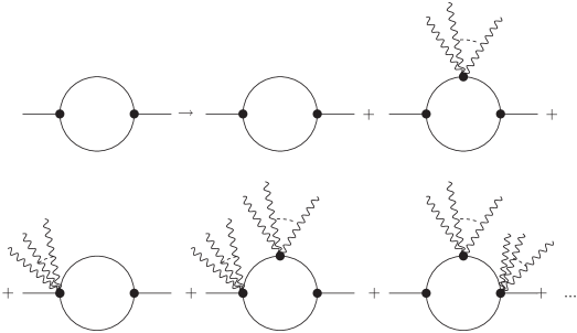
tails. An example of such set is depicted in Figure 1.
Due to the non-polynomial nature of gravity, every
flat-space diagram is producing an infinite number of
diagrams
with external tails, including an infinite
number of divergent diagrams. In order to establish the
structure of possible divergences, one has to impose
covariance which does not follow automatically from the
calculations. Then the number of relevant diagrams
becomes finite, making the analysis of renormalization
rather simple.
The shortcomings of this method are the lack of explicit
covariance, difficulties in practical calculations and
interpreting the results. However, there is a serious
benefit coming from the fact that, in the framework of
this method, we deal with the usual flat-space QFT.
According to the general theorems of the renormalization
theory (see, e.g., [125, 60] and
[131]) the divergences in QFT can be removed
by the local covariant counterterms. So, let us notice that
the necessary counterterms in curved space are local ones.
Figure 1: The straight lines correspond to the matter (in this case
scalar with
interaction) field, and wavy lines to the external metric.
A single diagram in flat space-time generates an infinite
set of families of diagrams in curved space-time.
The first of these generated diagrams is exactly the one in the
flat space-time, and the rest have external gravity lines.
The simplest of the known covariant methods is based on
the local momentum representation [34]. In
general, the use of momentum representation is not
possible in curved spaces, however one can use normal
coordinates (see, e.g. [98] for the introduction)
and perform loop calculations in the tangent space
corresponding to a given point .
One can express all quantities of interest, such as free
and interaction parts of the classical Lagrangian in form
of the power series in . Due to
the special choice of coordinates, the coefficients of this
series are components of curvature tensor and its covariant
derivatives in the point . The local momentum
representation can be used for both propagator and vertices
and finally enables one to derive local quantities such
as counterterms. For instance the first order expansion
for the propagator of a massive non-minimal scalar field
has the form
(37)
Similar expansions can be constructed for spinor and
vector fields and also for the interaction vertices.
Taking the locality of the counterterms into account
it is obvious that, after replacing such expansions
into Feynman diagrams, the structure of divergences
will be as follows. The zero order terms will produce
the divergences which are direct covariant generalizations
of the ones in flat space-time. Furthermore, the quadratically
divergent in flat space diagrams will produce logarithmic
divergences (and therefore counterterms) linear in curvature
tensor. Due to the dimensional reasons and gauge invariance,
there are only two types of such terms.
The first one is the Einstein-Hilbert type counterterm,
with the coefficient proportional to the square of the
mass of the quantum field. The second one is the non-minimal
scalar-curvature interaction term which really shows up
in the interacting scalar theory. Finally, in the next
order in curvature there will be the fourth derivative
counterterms. They can be constructed from the metric
only, because matter fields are dimensional. The most
important observation is that, if the original QFT in
flat space is a renormalizable theory, starting from the
third order in curvatures there will be only finite
contributions.
Let us notice that the locality of the counterterms
follows from the previous
approach
and from the universality of the vacuum EA.
The information provided by the two methods which we
briefly described above enables one to establish the
general structure of renormalization in curved
space-time. Another advantage is that these methods
can be applied at higher loops. However, for the
practical one-loop calculations we better apply
another approach.
Schwinger-DeWitt expansion [129] is the most useful
method for calculating divergences and related quantities.
The key point is the representation of the
via the proper time integral
(38)
(39)
are Schwinger-DeWitt
coefficients, while the expression for
has the form
(40)
Here is the geodesic distance between
and and
is the Van Vleck-Morett determinant. Further details of the
standard Schwinger-DeWitt technique can be found, e.g., in
[129]. A very powerful generalization, which enables
one to derive 1-loop divergences for a variety of quantum
theories on curved background and also for various models of
quantum gravity, has been developed in [15] (see
also references therein). A comprehensive review on the
effective action method and in particular generalizations
of the Schwinger-DeWitt technique has been recently given
in [124].
3.3 One-loop divergences and renormalization
In the framework of the Schwinger-DeWitt technique the UV
limit corresponds to the lower limit in the
proper-time integral (38). The regularizations of
this integral can be performed in different ways. The most
common is the special version of dimensional regularization
[27, 15], but one can use also
Zeldovich-Starobinsky approach [134], an
equivalent adiabatic regularization [89],
point-splitting [40] or even
covariant cut-off [7] regularizations. In the four
dimensional case the -coefficient of (38)
corresponds to the quartic diveregence and the
-coefficient corresponds to the quadratic divergence.
It is well-known that the cancelation of these divergences
may be related to the fine-tunings in imposing the
renormalization conditions. This may be lead to difficulties
in such cases as hierarchy problem in the Standard Model
or the Cosmological Constant problem (which is, actually,
also a hierarchy problem [110]) but we will not deal
with these issues here. The reason is that, despite the
fine tuning is unnatural, in the case of quadratic
or quartic divergences it has no apparent concern for the
form of quantum corrections which we are interested in.
The most important for us are logarithmic divergences
which are proportional to the “magic” coefficient
of (38).
The logarithmic divergences define such important notions as
renormalization group -functions and anomalies.
The form of in the vacuum sector is
(41)
where444We are introducing the double notations
. This will prove
useful in the sections devoted to conformal anomaly and
its applications.
(42)
Using these formulas, one can write the total expression for
the divergent part of the one-loop effective action of vacuum
for the theory involving real scalars, Dirac
spinors and massless vectors
(43)
In (43) we used the notations of dimensional
regularization, but of course the leading logarithmic
divergence is regularization independent.
Let us make a few observations concerning the expression
for the one-loop divergences (43).
i) The divergences have exactly the
form which follows from the general arguments presented
above. All high derivative terms of dimension four,
Einstein-Hilbert term and cosmological constant are
necessary to have a renormalizable theory of matter
on curved background. Let us remark that in case the
interacting scalar is present, the non-minimal term
is also necessary [31] (see the
references to the original papers therein).
ii) According to the consideration
presented above, at any loop order the divergences
of the gauge theory in curved space-time are of the
same form as the non-minimal classical action with
the vacuum term or, in other words, of the same
form as one-loop expressions. The only difference is
the coefficients of the divergent terms, which start
depending on the couplings at higher loops (see, e.g.,
[68]). Therefore
the theory formulated above is multiplicatively
renormalizable in curved space-time. At any loop order
the counterterms can be removed by renormalizing the
full set of parameters of the theory, including couplings,
masses, and vacuum parameters. There is no
need to renormalize the external metric field.
iii) The one-loop divergences are given
by an algebraic sum of the contributions from a free
scalar, fermion and vector fields. The reason is that,
as we have already mentioned above, each of the Feynman
diagrams which we take into account consists of
the single loop of a matter field with external tails
of a gravity field. No matter vertices show up
at this level.
iv) In the massless case only the higher
derivative counterterms emerge. This means the global
conformal symmetry holds in the one-loop divergences. As
we shall see below, however, this symmetry is violated in
the finite part of effective action.
v) The non-minimal parameter
affects the one-loop divergences, but it can be only
seen in the
combination . As we already know, the value
corresponds, in the massless case, to the
special version of the scalar theory which possesses the
local conformal symmetry.
Furthermore, the unique non-conformal counterterm,
in the massless case,
, has coefficient .
This means the one-loop divergences are conformal invariant
if the original theory is invariant. More precise is to say
that the four-dimensional coefficient of the pole term
satisfies the conformal Noether identity (18).
vi) All features described in the previous
points can be explained in a systematic way. But there
are some amazing things in the expressions (42)
which are still waiting to be explained. It is easy
to see that the contributions of scalars, fermions
and vectors to the -functions and
show a universality of signs. The ones to are
all positive and the ones to are all negative.
As we shall see later on, the universality of the signs
of has great importance for the Starobinsky
inflationary model. The mentioned sign rules have
nothing to do with the Grassmann parity of the fields
and remain an unexplained occurrence. It is even more
mysterious that the higher derivative conformal fields
(scalars and fermions) constructed so far
[100, 54, 21] always produce opposite
signs (compared to the usual scalar, fermion and vector)
of the contributions to both -functions.
vii) Coming back to the heat kernel
expansion (39) one can notice that the finite
terms start from
and have the form of local covariant expressions with
growing powers of metric derivatives. For instance,
has the -type and
-type terms. The general expressions
are known for and
[59, 10].
3.4 scheme - based
renormalization group
One can use the multiplicative renormalizability of the
QFT in curved space-time to formulate the renormalization
group equations for all quantum fields and parameters.
As usual, the simplest version of the renormalization
group can be constructed in the framework of the minimal
subtraction () renormalization scheme
[86, 32, 119]. The detailed exposition
of the scheme - based renormalization
group method in curved space-time can be found in [31].
Here we shall only give brief account of this method.
Consider the quantum theory of the fields on the
background of classical metric . The full
set of parameters of the theory will be denoted by .
For example, in case of SM or GUT - like QFT,
includes fermions, Yang-Mills fields and scalars and
includes gauge, Yukawa and scalar self-interaction
couplings, non-minimal parameters and the
parameters of the vacuum action (12),
including Newton and cosmological constants.
The dimensions of and will be denoted
as and , correspondingly.
For the sake of definiteness we assume the dimensional
regularization. The -scheme
renormalization group equation for the effective action
means that the last is independent on the dimensional
renormalization parameter
(44)
where we used the standard notations for the renormalization
group and - functions in -dimensional
space-time
(45)
while the usual -functions correspond to the limit
.
Let us notice that these formulas are essentially the
same as in the flat space-time. The main difference is
the presence of , playing the role of
external parameter. As a result there are several
qualitatively new effective charges, such as and
vacuum parameters.
The eq. (44) is a formally universal renormalization
group equation which can be used for different purposes,
depending on the physical interpretation of . For
example, in order to consider the short distance limit,
we can perform a global rescaling of all quantities,
including metric and obtain another identity, which is
independent on (44)
(46)
After being considered together, (44) and (46)
produce the general solution of the form
(47)
where the effective charges and
satisfy the renormalization group equations
(48)
The limit corresponds to the short
distances and, due to
(49)
to the limit of greater curvatures. In this respect it
is equivalent to the standard rescaling of momenta in the
flat-space quantum field theory. On the other hand,
the application of (47) and (48) to
particular situations needs a special attention. For
example, let us consider the exponential inflation.
The time-dependence of the metric
(50)
looks similar to the rescaling (47). However,
inflation does not fit the -based
renormalization group, because the scalar curvature
does not behave according to (49).
The origin of the difference is that the
parameter of the global rescaling is a
constant, while the time in (50) is a
coordinate and therefore the transformation (50)
is a local one.
In order to understand the physical significance of the
renormalization group running in curved space one has
to attribute some physical sense to the parameter .
At this point one has several option. Let us
formulate the above question in a different way: which
terms in the effective action can be parametrized by
the -scheme renormalization group
in curved space? Remember that the standard
interpretation of the -scheme
renormalization group in flat space is related to the
high energy limit in the momentum subtraction scheme
of renormalization. In this case, in order to get the
terms in effective action which are behind the
renormalization group, one has to replace
by the expression
, where is the square of the
momentum. In the coordinate representation this means
we have to introduce the formfactor
.
For example, in case of QED, the corresponding term
looks like
(51)
This procedure can be indeed generalized to the case of
a curved space. The expected term is, for instance,
(52)
for the case of the Weyl term in the action of
vacuum (12). Of course, the d’Alembertian
operator in (52) is the covariant one.
Later on, in section 6, we shall confirm the
presence of the term (52) by a direct
calculation [61]. The -scheme
based procedure described above can be successfully
applied to derive the quantum corrections to the
classical action of gravity and, e.g., scalar field
[33, 31] (see also [45] for an
alternative consideration). At the same time, this approach
meets obvious difficulties when applied to the running
of the Newton or cosmological constants
[61, 14, 85].
In these cases the formfactor can not be simply inserted
into the action, because the d’Alembertian operator acting
on the cosmological constant gives zero. Similarly, in
the Einstein-Hilbert term, the formfactor can only produce
the total derivatives, or superficial terms, which do not
affect the equations of motion for gravity. We shall
come back to these arguments in section 7.
Can we state that the identification of with
is a universal tool making the
-scheme results physically relevant?
Unfortunately, the problem is not really solved by the
analogy with QED, because in gravity, according to the
relations (49) one can identify with
other metric-dependent quantities.
For example, the scalar curvature has the same global
scaling law as the d’Alembertian operator . In this
way we can construct the curvature-controlled version of
renormalization group. It is interesting that the
corresponding expressions in the effective action
can be also obtained by special resummation of the
Schwinger-deWitt series
[90, 91]. From the general
perspective the identification of with the
scalar curvature is as legitimate as its identification
with and moreover it has the following two
advantages: the possibility to write down the quantum
correction to the cosmological and Newton constants and
the closeness to the most natural identification of
with the Hubble parameter in the cosmological
setting [11, 111]. One has to
remember, however, that anyone of these identifications
is no more than a particular model for an unknown
complete effective action. An obvious manifestation
of this feature is a vast ambiguity which one
meets in the resummed and truncated expressions used
in [91].
It is important to remember that the renormalization
group is a method to parametrize the scaling dependence
of the effective action.
In case of gravity it is especially difficult to introduce
a physically consistent and universal renormalization
group, in particular because definition of the energy
of the gravitational field is a nontrivial problem
(see, e.g., [44] and references therein).
The solution of the renormalization group equations
(48) has been explored for different QFT models
in curved space [31] (see further references
therein). The equations for
couplings and masses of the quantum matter fields are
exactly the same as in flat space-time [39].
The qualitatively new elements are the equations for
the nonminimal parameters and for the parameters
of the vacuum action .
The one-loop is always proportional to
the difference , such that the conformal
value is a universal fixed point of the
renormalization group trajectory in the theory with
scalar fields. The coefficient of proportionality
depends on the model. For some gauge models it
leads to the UV asymptotic conformal invariance
[28] and for other models the conformal value
is the IR fixed point. The general conditions for the
asymptotic behavior of have been found in
[29]. Indeed at higher loops the
is not proportional to factor anymore
[68]. The related ambiguities lead to
the quantum inconsistency of the conformal invariant
theory [7] beyond the one loop approximation.
Finally, there is one subtlety in the physical
application of the renormalization group equations for
the cosmological and Newton constants (42)
(53)
Do we need the second terms in the r.h.s. of these
two equations? In order to address this question one has
to remember that and gain physical sense when
they are inserted into the Einstein equations
(54)
The second terms of (53) reflect the classical
dimension of and , but other components of
(54) also have their own dimensions. As a
result the classical scaling terms do cancel and, for
the applications, one has to use only anomalous
dimensions, that are the -functions terms.
4 Conformal anomaly and anomaly-induced EA
In general, there is no way to calculate the vacuum effective action
completely. In order to understand why this is so, let
us remember that already in the Schwinger-DeWitt expansion
we observe an infinite series in curvature tensor and
its derivatives. On the top of that, the renormalization
group and analogy with QED indicates, as we have
discussed in the previous section, the presence of
an infinite amount of non-local insertions. So,
the task of deriving the full effective action does
not look realistic. It is remarkable that there is a
class of the four-dimensional theories for which we are
able to derive exactly the non-local terms in
. The word “exactly” here
means we can do it at the one-loop level and only
on the very special backgrounds. Despite of
these restrictions, the situation deserves this wording,
as a way to emphasize an enormous difference
with the situation typical for other kinds of theories.
In this section we consider the anomalous violation
of local conformal symmetry in the case of quantum matter
on classical curved background. The conformal anomaly
enables one to derive the anomaly-induced effective
action. In the consequent section we shall discuss the
applications of anomaly and of the induced effective
action.
4.1 Derivation of conformal anomaly
Quantum anomaly is a typical phenomenon in a situation
where the original theory has more than one symmetry.
The origin of anomalies is the renormalization procedure
[97]. The anomaly shows up if there is no
regularization which preserves all symmetries at the
quantum level. After the divergences
are subtracted, in the finite part of the effective
action some of the symmetries are getting broken. In
our case the theory has general covariance and local
conformal symmetry, and the last is broken by quantum
corrections.
Consider quantization of free massless conformal
invariant matter fields denoted by , on classical
gravitational background. As before, we assume that the
set of quantized matter fields includes
scalars (all with ), fermions
and vectors. We denote the
conformal weight of the field.
At the one-loop level
it is sufficient to consider the simplified vacuum action
(55)
Let us emphasize that it is not wrong to supplement the
last expression by the Einstein-Hilbert action, cosmological
constant or the -term. The action
(55) can be seen as a part of classical
action which is a subject of an infinite renormalization
at the one-loop level. Beyond the one-loop approximation
the term is also necessary,
because the conformal theory becomes inconsistent
[7].
The Noether identity for the local conformal symmetry has
the form (18) and can be interpreted as
on shell (see section 2).
At quantum level has to be
replaced by the effective action of vacuum
. As we already know, its
divergent part is
(56)
where in dimensional regularization.
In the case of global conformal symmetry, the renormalization
group method or -regularization tell us
[69, 32, 31]
(57)
where . In the case of local conformal
invariance there is an ambiguity in the parameter
[25, 48, 6]. This issue has been explained
recently in [7] and reviewed in [106],
so we will not discuss it in full details here. Qualitatively
the result is that the ambiguity is always equivalent to
the freedom to add the -term to the
classical action.
One can derive the conformal anomaly in different ways,
mainly due to the choice of regularization schemes
[49, 40, 25, 7]. We shall follow
[49] and [7, 106], using dimensional regularization. We are interested in the vacuum effects
and therefore, at the one-loop level, can restrict
consideration by the free fields case. The expression
for divergences is (56) with the -functions
defined in (42).
The renormalized one-loop effective action has the form
(58)
where is the naive quantum correction to the classical action and
is an infinite local counterterm which is called to
cancel the divergent part of (56).
Indeed is the only
source of the noninvariance of the effective action, since
naive (but divergent) contributions of quantum matter fields
are conformal. The anomalous trace is therefore equal to
(59)
The calculation of this expression can be done, in a most
simple way, as follows.
Let us change the parametrization of the metric to
(60)
where is the fiducial metric with
fixed determinant. There is a useful relation
(61)
At that point we need transformation laws for the
structures presented in (56). They can be found,
for instance, in [38], so we will not reproduce
these formulas here. For instance, for the square of the
Weyl tensor we have
(62)
All other expressions of our interest (56) have
the same factor and, on the top of that,
some extra terms with derivatives of . For all
terms which are not total derivatives, these terms are
irrelevant due to the procedure (61).
In the simplest case of global conformal factor
we immediately arrive at the expression
(57) with . However in the local
case the situation is more complicated.
It is worth mentioning that the left hand side in
(61) gives zero when applied to the integral
of the total derivative term .
On the other hand, the value of can be
modified by adding a finite term
The last formula can be derived either directly or through
the eq. (61). The same effect can be achieved by
the term ,
(65)
and also by the term .
For the sake of simplicity, below we shall discuss only
the term .
One may think that adding the classical non-conformal term
(63) has nothing to do with the quantum corrections.
However, consider in more details how to apply the procedure
(59) to the counterterm of the
-type. The point is that the Weyl tensor
depends on the dimension , in particular its square is
(66)
When defining the corresponding counterterm
(67)
one can choose the Weyl tensor with ,
where is an arbitrary number. For any such the
counterterm is local, it cancels the divergent part of
effective action and the renormalization is multiplicative
in the , and
basis. However, the anomalous term depends on
the choice of . Hence at this point we meet an
arbitrariness. The particular choice has been
done in [49]. In this case we arrive at
(68)
For scalars and spinors the result is identical for the
global and local conformal symmetries violation. In case
of vectors there is no such equivalence and, moreover,
this is only one particular case of the possible
counterterms.
Finally, it is easy to see that the difference between
the counterterms (67) with different is equivalent
to the finite -term. Qualitatively
similar ambiguity takes place in the covariant Pauli-Villars
regularization [7]. Finally, the anomaly is given
by (57), but there is an ambiguity in the
coefficient . If most of regularization
schemes but, in general, fixing
this coefficient requires a special renormalization
condition [6, 106].
4.2 Anomaly-induced action
One can use conformal anomaly to construct the equation for
the finite part of the 1-loop correction to the effective
action (the notations are according to (42))
(69)
The solution of this equation is straightforward [100]
(see also generalizations for the theory with torsion
[35] and with a scalar field [108]).
Here we shall follow a bit more detailed exposition
given in [106].
The simplest possibility is to parametrize metric as in
(62), separating the conformal factor
and rewrite the eq. (69) using (61).
The solution for the effective action is
(70)
where is an unknown
functional of the metric, which serves as an integration
constant for the eq. (69).
The merit of the solution (70) is its simplicity,
but it is not covariant or, in other words, it is not
expressed in terms of original metric . It
proves useful to obtain the covariant solution [100, 107].
Let us establish the following relations [100]
(see also [38] for details):
(71)
(72)
where is a fourth derivative conformally
covariant operator acting on dimensionless scalar
(73)
and also introduce the Green function for this operator
.
Using these formulas and (61) we find, for any
, the relation
(74)
Using this relation it is easy to find the term in the effective
action, which is responsible for ,
(75)
Similarly one can find the term which
produces
(76)
The third constituent of the induced action follows from
eq. (64)
(77)
The covariant solution of eq. (69)
is a sum of the expressions (75), (76)
and (77).
The anomaly-induced action presented in a local form using
auxiliary scalar fields. After
using the classical equations of motion for these fields
and replacing them back to the action we come to the
original non-local expressions.
In order to construct the local covariant representation,
the action should be presented in a symmetric form
(78)
The last two terms are appropriate objects for rewriting them
using the auxiliary fields. In this way we arrive at the following
final expression for the anomaly generated effective action of
gravity.
where
(80)
Some important remarks are in order.
1) The local covariant form (4.2) is dynamically
equivalent to the non-local one (78), (77).
The complete definition of the Cauchy problem in the theory
with the non-local action requires defining the boundary
conditions for the Green functions , independently
in the two terms (75) and (76). The
same can be achieved, in the local version, by imposing the
boundary conditions for the two auxiliary fields and
.
2) The local form of effective action with two auxiliary
scalars (4.2) has been introduced in the paper
[107]. Qualitatively similar manner of introducing second
scalar has been suggested later on in [79].
The kinetic term for the auxiliary field is positive
while for it was negative. For the kinetic term
has negative sign. The wrong sign does not lead to problems
here, because both fields are auxiliary and do not propagate
independently.
3) We introduced the new structure
into the action, despite it
was not directly produced by anomaly. This term is indeed
conformal invariant and therefore its emergence may be viewed
as a simple redefinition of the conformal invariant functional
. On the other hand, writing the non-conformal
terms in the symmetric form (78), we have modified
the four point function in a very essential way. Therefore,
introducing the mentioned conformal term we have just restored
the basic structure of the terms generated by anomaly. For this
reason, the second auxiliary scalar [107]
represents a natural element of writing the induced action
in a local form.
4.3 Light massive fields
Before we start to discuss the applications of conformal
anomaly and of the anomaly-induced action, let us show
how the same approach may be useful for exploring the
effective action of light massive fields. In section 6
we shall also consider the case of heavy massive fields.
In order to understand why these two cases must be treated
separately, let us come back and look at the Schwinger-DeWitt
expansion (39). It is easy to see that it
corresponds to the growing powers in metric derivatives.
Due to the covariance, this is actually an expansion in
the positive powers in curvatures and their covariant
derivatives. The dimension is compensating by the
negative powers of the mass of the quantum field.
Indeed, such expansion is going to be efficient is
the curvature invariants are much smaller than .
In other
words this is an approximation for the “heavy” fields
case. However, there are physical situations where we
need another approximations, for instance for the case
of light fields, where curvature invariants satisfy
, or for an intermediate
regime, where these two quantities are of the same order
of magnitude. It is remarkable that we have no regular
approximations for these two cases and, in the last
case, there is no available method at all. However, for
the light fields, there is one method, suggested in
[108] and slightly generalized in [95].
Let us consider the theory where the conformal invariance
of scalar and fermion actions is violated only by the
masses of these fields and by the Einstein-Hilbert
action. The idea is to treat the masses as
perturbations with respect to the massless theory.
Originally, there is no local conformal symmetry and hence
one can not use the conformal anomaly to derive quantum
corrections. But, this can be changed if we apply the
conformal parametrization of the massive theory. The
transformation is similar to the one used long ago
in the cosmon model [93] and in GR [42].
The calculations perform in the following three steps:
1) Conformization of the theory;
2) Derivation of anomaly and
anomaly-induced effective action of the new theory;
3) Coming back to the original parametrization.
Let us replace the dimensional parameters in both matter
and gravitational sectors by the powers of a new auxiliary
scalar field according to
(81)
Here is a new dimensional parameter.
In order to provide the local conformal invariance we
postulate that the auxiliary field transforms as
. Under
the procedure (81), the massive terms for the
matter fields are replaced by Yukawa and scalar
interactions involving the new auxiliary
scalar . The new action is conformal invariant
in both matter and gravitational sectors. The
classical Noether identity for the new vacuum action
has the form
(82)
The conformal invariance is violated by a conformal
anomaly and one can derive the effective action of the
background fields using the
anomaly-induced effective action scheme.
The divergences of the theory in the conformal
representation have the form
(83)
where the coefficients and are given by Eq.
(42) and
(84)
Here the sums are taken
over massive fermion and scalar fields with
the masses and correspondingly,
and being multiplicities.
The conformal anomaly is proportional to the integrand of
(83)
(85)
In the standard way, described in section 5.1, one can
derive the anomaly-induced effective action of the background
fields and
(86)
The last step is to fix the conformal unitary gauge
, such that the
classical Einstein-Hilbert and cosmological terms acquire
their standard form
Let us discuss the level of reliability behind the
calculation of the effective action
(4.3). First of all, it is easy
to see that this is not an exact result, even for the
FLRW-like metric. The reason is that the integration
constant in (86)
depends on the intermediate scalar and, after
fixing , is not
conformal invariant functional anymore. The second
observation is that the higher-derivative part of the
Eq. (4.3) is identical to that for
the massless fields. Let us remember that the one-loop
effective action is given by
of some operator, depending on the background metric
[130]. The can be seen
as a product of the eigenvalues of the operator
, depending on the corresponding
eigenfunctions (see, e.g., [50]). When we
are adding the masses of the fields, there are two
distinct effects: modified eigenvalues due to the
masses and also modified eigenfunctions. It is
obvious that the calculation presented above takes
into account only the first effect, that is why the
higher derivative sector does not change. Perhaps
the second effect manifests itself in the
-term, but this part is out of
our control.
In order to understand better the approximation which
is assumed in our calculus, let us notice a strong link
between the anomaly-induced effective action
Eq.(4.3) and the quantum
corrections coming from the renormalization group.
The expansion of the homogeneous, isotropic universe means
a conformal transformation of the metric
.
On the other hand, the renormalization group in curved
space-time corresponds to the scale transformation of the
metric
simultaneous with the inverse transformation of all
dimensional quantities [31]. For any we
have . One can compare the
-dependence of the anomaly-induced effective
action (4.3) and the
-dependence
of the renormalization-group improved classical action
(88)
where denote
vacuum parameters of the theory and .
The expression (88) is a leading-log
approximation for the solution of the renormalization
group equation for the effective action [31]
(89)
where are matter fields.
It is easy to see that (4.3) becomes
completely equivalent to (88) if we set .
The coefficient is a factor of the -function
for the inverse Newton constant and the
coefficient is a factor of the -function for the
cosmological term . Indeed, (89) can be
considered as a generalization of the renormalization group
improved classical action (88). After all, one can
consider Eq. (4.3) as a leading-log
approximation for the effective action for the massive fields.
This approximation
picks up the logarithmic quantum corrections and is reliable
in the high energy region where masses of the fields are much
smaller than the Hubble constant . The anomaly-induced
expression may be even seen as a -scheme
based local version of renormalization group [113],
but the consistent formulation of such local renormalization
group is not available yet.
5 Applications of the anomaly-induced action
The most important areas of application for the quantum
corrections to the action of vacuum are cosmology and the
black-hole physics. In both cases the anomaly-induced
effective action described in the previous section
is behind the most well-established results, such as
Hawking radiation and Starobinsky model of inflation.
In this part of our review we shall give a very
brief account of these two subjects. We shall
follow the original publications [12, 52, 95]
where one can find more detailed considerations.
5.1 Vacuum states in the vicinity of a black hole
At the classical level, the black hole does not emit
radiation, but such emission can take place if we
take quantum effects into account.
After the theoretical discovery of the black hole
evaporation by Hawking [70], the same
result has been obtained from analytical estimates
of for matter fields
propagating in a fixed static Schwarzschild black
hole geometry. Indeed, the black hole evaporation
phenomenon has not been confirmed experimentally.
In the situation when the complete information on the
vacuum state or, equivalently, on the effective action
of vacuum is unavailable, one can not be absolutely
certain that such evaporation really takes place.
However, all known
methods converge predicting such quantum radiation.
The completely consistent approach would involve the
simultaneous solution of the following two problems:
solving equations of motion derived from the effective
action and derivation of the quantum evaporation of
the black hole. However, the practical calculations
which have been performed so far, are based on the
reduced approach, when the quantum effects are
estimated on the background of the purely classical
solution. Here we shall use the same approximation
[12].
The idea to derive the Hawking effect starting from
the effective action of vacuum is natural.
The main problem here is to choose the appropriate
method for evaluating the effective action. For
example, in [84] (see also [13])
the starting expression has been derived starting
from the two-dimensional conformal anomaly in the
dimensionally reduced (from ) theory. As a result
there are serious difficulties and the fit to the standard
result requested some artificial procedure related
with introducing an effective potential of the
conformal factor of the metric. Similar situation
takes place in recent works [123], where
the consideration was based on a new complicated
approach to deriving the effective action of vacuum.
Let us notice that no one of existing techniques for
the effective action of vacuum is perfect in a sense
there is always an ambiguity. The unique case when
we can arrive at the exact one-loop result is the
conformally trivial (e.g., FRW) metric, but this is
definitely different from the black-hole situation.
Then, since it is known the Hawking effect is closely
related to the four-dimensional conformal anomaly
[41], it
is natural to expect the best fit with the traditional
methods if starting from the anomaly-induced effective
action. Indeed, this approach really enables one to
classify the vacuum states in a somehow clear way and
reproduce the standard result for the Hawking
radiation [12]. Moreover, the analogy with
the black hole vacuum turns out to be very fruitful
for the investigation of the gravitational waves in a
anomaly-induced background [52], where we achieve
a close fit with the well known result of [114]
and with the consequent calculations [72].
Consider the application of the anomaly-induced
effective action (4.2) to the analysis of
the quantum effects in the vicinity of a black hole.
We shall see that the different vacuum states of the
black hole (Boulware,
Hartle-Hawking and Unruh) correspond to the different
choices of initial conditions for the two auxiliary fields
[12]. The result can be generalized for the
Reissner-Nordstrom spacetime case [4].
Let us stress that such classification can not be
accomplished by using only one field . Therefore the
correspondence with other approaches to Hawking radiation
confirms that our considerations about introducing the
second auxiliary scalar are correct.
Detailed analytical and numerical investigations,
based on the analysis of
in the classical black hole background have been
performed in [37]. One of the fundamental
properties of this background is the existence of
three different vacuum quantum states, which are
defined as follows:
i) The Boulware vacuum [26] is
obtained by choosing in and out modes to
be positive frequency with respect to the Killing
vector of the Schwarzschild metric
(2).
This state reproduce the Minkowski vacuum
asymptotically, in the limit we find
.
At the same time the behavior of the same average
value on the horizon is divergent in a free
falling frame. In this situation, for the classical
observables, one can choose another coordinates, e.g.
(4), such that the horizon becomes free of the
singularities. In quantum theory this corresponds to
choosing another vacuum state.
ii) For the Unruh vacuum [120] the
in modes have positive frequency with respect
to , while the out modes are taken to
be positive frequency with respect to Kruskal’s
(4). The value
is regular on the
future event horizon but not on the past one.
Asymptotically in the future
has the form of a
flux of radiation at the Hawking temperature
. Hence this vacuum state
is the most appropriate to discuss evaporation of
black holes formed by gravitational collapse of
matter.
iii) The Israel-Hartle-Hawking vacuum
state [66] is obtained by choosing in
modes to be positive frequency with respect to the
Kruskal’s coordinate and out
modes positive frequency with respect to the affine
parameter along the past horizon.
for
describes a thermal bath of radiation at the Hawking
temperature .
This vacuum state corresponds to a black hole in
equilibrium with a surrounding thermal bath.
Asymptotically both in the future and the past
.
The existence of three distinct vacuum states in quantum
theory looks natural, in sense they reflect distinct
choices of coordinates systems and construction of
different in and out modes with respect
to the corresponding coordinates. The main difference
between classical and quantum theories is that, in
the first case we know how to transform the coordinates.
So, the natural question is how to perform the transition
between different vacuum states ,
and ?
The anomaly-induced part of the effective action do not
make any reference to a particular quantum state. Therefore
one has to look for the non-universal part of effective
action in order to implement one or another state.
We remember that the solution (78) is exact
only for the conformally-trivial metric, such as the
Friedmann-Robertson-Walker (FRW) one.
In all other cases the conformal invariant functional
is a source of uncertainty.
Furthermore, in order to apply the
quantum correction (4.2) one has to fix
the extended set of boundary conditions, including the
ones for the auxiliary scalar fields and
. It turns out that the identification of the
Boulware and Unruh vacuum states can be performed, in
the leading approximation, by choosing an appropriate
initial and boundary conditions for the auxiliary
scalars. In order to achieve the Israel-Hartle-Hawking
one has to make an additional adjustment of the
conformal functional. We will not go into details
here, because one can easily find them in [12]
(see also [13] where the more simple
effective two-dimensional case has been treated)
and present just the list of main results.
The equations of motion for the auxiliary fields
and have the form
(90)
where we used the notations (80). In the Ricci-flat
space the operator boils down to , such that
we get
(91)
where . The equation for
can be obtained by trading . Until the
end of this subsection we shall set the Newton constant
. It proves useful
to introduce the traceless tensor (an
explicit form of this object can be found in [12])
(92)
then
(93)
where we omitted those term which vanish on the Ricci flat
background such as the Schwarzschild metric. Let us notice
that represents only that
part of the average Energy-Momentum Tensor which can be
restored from anomaly, being in general different from
the unknown complete quantity .
The strategy for identifying the given vacuum state is as
follows. One solves the equations (90) for the
auxiliary fields and replace the solutions into (93).
These solutions will always depend on the set of integration
constants and one can try to find the “correct” ones to
identify
for the given
vacuum state , being it
, or .
The general solution for has the form
,
where satisfies the equation
(94)
and are constants that specify the homogeneous
solution and hence the quantum state. For
we have a similar solution, but with another set of
integration constants . It is important
that these two sets are independent on each other, due to
the independence of and .
In the case of a Boulware state we request
when .
For the auxiliary scalars in the Minkowski vacuum we
can safely set . This asymptotic conditions
and also cancelation of singular terms in the solution
of (94) enables one to fix all constants and we
arrive at the asymptotic expressions [12]
(99)
for and
(100)
This behaviors perfectly reproduce the one which is
observed in the framework of other methods [37].
Namely, we have
in the space infinity and the quadratic divergence
near the
horizon in the Boulware case.
Another success of our method comes in the case of
the Unruh vacuum. Using the same treatment of auxiliary
fields, but choosing another values of the constants
and , we meet, near the
horizon, the following asymptotic behavior [12]:
(103)
which is regular on the future horizon. The asymptotic
form at the space infinity is
(108)
The results of eqs. (103), (108) are
in exact agreement with the standard ones on
Hawking radiation [37, 130], once the
luminosity of the radiating black hole is identified
with
(109)
A little bit more complicated situation takes place for
the Hartle-Hawking vacuum, where one should not only
properly choose the initial conditions but also fine-tune
the coefficient to order to achieve correspondence
with the results achieved by other methods. From the
general perspective this situation looks somehow natural
because, as we already explained earlier, the unknown
conformal invariant functional is relevant for
the spherically symmetric metric. The modification of
is nothing else but the adjustment of . So,
we can consider as a kind of luck that the most
essential part of the classification of the vacuum
states can be performed by the use of the initial
conditions for and , such that only
in the case of we are forced to modify the
conformal term.
5.2 Modified Starobinsky model.
Another interesting application of the
anomaly-induced action is the Modified Starobinsky Model
or anomaly-induced inflation [52, 108, 95].
Let us follow [108, 95] and first consider
quantum effects of massless fields, that is use the
effective action (70). At the second stage
we shall take masses of the fields into account, that
means we shall use the action (4.3).
As a first step consider an empty space, when matter is
absent. There are two equivalent ways to arrive at the
cosmological solution of the theory with quantum
corrections: using the --component
[53, 114] or via the anomaly-induced effective
action [35, 31]. Let us choose the last option.
The resulting equation has, for FRW metric,
the following form555The cases are
quite similar [95] and we do not consider them
here.:
(110)
where the coefficients are defined in
(42). The last equation does
not depend on the coefficient , because the
Weyl tensor vanish for the FRW background.
The equation (110) has a remarkable particular
solution
(111)
where
(112)
As far as , we meet two very different
values of (we consider )
(113)
The solution with is the one of the theory without
quantum corrections. The second value corresponds
to the inflationary solution of Starobinsky [114].
Let us notice that the sign of is negative
independent on the particle content (42).
Let us remark that the
expression “particle content” here corresponds to the
degrees of freedom contributing to the vacuum effective
action in the virtual loops and has nothing to do with the
matter content of the universe.
Further understanding of the inflationary solution
requires analyzing its stability properties.
The phase portrait of the theory may look very different
depending on the sign of the coefficient , that is on
the coefficient of the local -term
[114, 95].
The inflationary solution is stable for a positive
and is unstable in the case . In the last case there
are several stable points (attractors),
one of which corresponds to the usual
solution. It is interesting that the
existence of the exponential solution is possible due to
the non-local and universal -term in the
anomaly-induced effective action, while the stability
depends on the local -term only.
The Starobinsky model looks appealing, in particular
because it has a solid QFT background and there is no
need to introduce a special inflaton field. The original
model [114] is based on the unstable solution .
In this case one has to choose the initial conditions in
a very special way. First of all, the initial point must
be very close to the exact exponential solution
(111),
such that the inflation lasts long enough. Moreover, one
has to provide that, after
the inflationary phase ends, the Universe will approach
the attractor corresponding to the FRW solution, and not
to other, physically unacceptable, attractors. All the
matter content of the Universe is created after the
inflation ends through the decay of the massive degree of
freedom induced by anomaly. Many interesting aspects of
this model, including gravitational waves and problem of
singularities, has been investigated starting from the
papers [114, 122, 3]. The first investigation
of inflationary density perturbations has been also
performed for this model [82].
An alternative way to use the solution (70)
[52] is based on a positive value of and
therefore on the stability of the exponential solution
at the beginning of inflation. It turns out that the
stable inflation is very robust with respect to the choice
of initial data [95], providing the following
two advantages: First, one does not need to consider an empty universe
in the initial state, since the stable inflation “kills”
any matter content in a few Planck times [96].
Second, there is no problem with the
unphysical solutions of the “run-away” sort, the
measure of the corresponding initial data is infinitesimal
for .
The real problem of the stable inflationary
model is to understand the period when the inflation
ends. If we stay within the original framework
[53, 114], that is consider only massless conformal
fields, the stable inflation will be eternal. The modified
Starobinsky model solves this problem using the effective
quantum field theory approach [108] and in
particular the notion of decoupling.
Using the relations (42), the condition of stability
can be cast into the form
(114)
The inflation is stable if there are many
scalars and fermions, for a given amount of vectors.
We know that in QFT vectors are responsible for the
fundamental interactions. It is easy to see that the
inequality (114) is not satisfied for the
MSM with . However, it
is satisfied for the MSSM with .
The same must be true for any realistic supersymmetric
model, because the supersymmetrization of the realistic
model implies transformation of fermions and scalars
into chiral superfields and vectors into vector
superfields. Both operations require adding many spinor
and scalar superpartners (sparticles) while the vector
sector of the theory remains the same.
The transition between stable and unstable inflation
can be associated with the soft SUSY breaking. Within
this approach the sparticles are supposed to be very
heavy compared to the usual particles. The inflation
becomes unstable when the typical energy becomes smaller
than the mass of the sparticles and they decouple.
As before, we associate the typical energy with the
Hubble parameter . Let us denote the
energy scale where the
inequality (114) changes its sign to the
opposite. The value is now seen just as
initial value of and is the final
point of the stable inflation. The transition occurs at
the instant which
is defined as a solution of the equation .
The details of decoupling will be considered in the next
section. The next problem is to find why the inflation
slows down. In fact, this can be discovered at once if
we take the masses of the fields
into account and use the result (86). The
equation of motion for has the form
(115)
where we introduced useful notations
(116)
The leading terms in the eq.
(115) are the same as in the massless case
(110), but the Planck mass and the cosmological
constant to be replaced by the variable expressions
(117)
(118)
Let us assume that, because of
supersymmetry, the quantum loops contributions to the
cosmological constant do cancel
[95].
Furthermore, itself is negligible at the energy
scale of inflation. Then the solution
of equation (115) can be obtained by
solving (117) in the form
(119)
The numerical analysis confirms the parabolic dependence
(119) with excellent precision [95].
The total number of the inflationary
-folds for different models of the SUSY breaking
can be obtained from the relation (119).
For example, in the case of MSSM we have ,
then and
the total amount of inflationary -folds is .
One can use the effective QFT approach to perform additional
tests of quantum corrections (70). If we believe
to the decoupling idea, the present-day Universe looks like
a perfect object to apply the effective approach. In the present-day Universe only the photon should be treated as
an active physical degree of freedom and hence, according
to (114), . Then the explicit analysis
of stability performed in [95], shows that the
solution in eq. (113) is stable if .
Furthermore, an additional advantage of the anomaly-induced
is the moderate behavior of the gravitational waves or, in
other words, restricted production of gravitons [52].
Until
now we could see only good points of the anomaly-induced
inflation. This model is completely based on the QFT results,
it does not require introducing new artificial entities such
as inflaton, does not require fine tuning for the action or
for initial data, moreover the gravitational waves do not
grow too much during the stable phase, making consistent
the whole approach based on the homogeneous and isotropic
metric. Unfortunately, there is also a real problem with
this model. As we already know, the total
amount of the inflationary -folds is enormous.
However, only the last of these -folds
are physically relevant. In order to extract the physical
information one needs, therefore, an effective action
in the region
when . However, as we have already discussed
above, we have no approximation for this situation,
which lies between the light-mass and the heavy-mass
extremes. No model exists for the intermediate situation.
Until such model will be constructed, the only way to
study inflation is through the inflaton approach.
However, the very fact that the inflation can be explained
by quantum effects of matter fields surely looks
interesting and greatly increase the importance of the
further study of effective action of massive fields.
6 Effective action for massive fields
For a while we have seen that two kinds of information
are available about the effective action in curved space.
First, we can completely calculate the divergences and
remove them using the renormalization procedure. The
procedure works perfect in curved space-time, independent
on that we do not have access to the complete expression
for the effective action or, equivalently, can not obtain
the vacuum state of the quantum fields on a classical
gravitational
background. The key point is that the divergences are
given by the well known local expressions and the unknown
part of the
effective action is non-local. Second, we are able to
obtain the non-local part within the anomaly-induced scheme.
In this section we shall go further and obtain, in a regular
way, some non-local terms for the massive fields theory.
We shall present only the main results here, the details
can be found in the original papers [61, 20].
Figure 2: The one-loop diagrams contributing to the
polarization operator of gravitons. The matter
field loop is connected to external gravitational
fields represented by wavy lines.
6.1 Decoupling theorem for gravity
As we learned above, the vacuum divergences can be
removed by the renormalization of the action
(12). This procedure leads to the
scheme - based
renormalization group running, which enables one to
restore the high energy asymptotics of the effective
action by trading by
[33, 31]. Now we ask the following questions:
are these terms really there? And what
happens at low energies, when the
scheme does not work? We know that in QED the main
phenomenon at the low-energy regime (we shall call
it IR) is the decoupling of massive fields [9].
One can expect something like that in the vacuum
gravitational sector, because the general structure
of the Feynman diagrams is similar (see, e.g., Fig. 2).
The most obvious way to the decoupling theorem is to
derive the effective actions and the -functions
through the
expansion
approach [61]. This method opens the way for the
momentum-subtraction renormalization scheme, that is
the standard approach for the Appelquist and Carazzone
theorem [9].
A useful alternative to the flat-space expansion is
a resummation of the Schwinger-DeWitt series,
culminated in the heat kernel solution of [16].
The results obtained within these two methods coincide
[61],
and for the scalar field we arrive at the following
result in the approximation:
(120)
Here is the parameter of dimensional regularization
It is easy to see that the divergences are exactly the
same as in the scheme (43),
(42). The qualitatively new part is encoded into
the formfactors (nonlocal insertions produced by quantum
corrections), which have the form
(121)
Here we used notations
(122)
Similar expressions can be found for massive fermion and
vector loops [61] and also for the scalar field
background, where the formfactors can be obtained for the
and terms.
In principle, there is a possibility to obtain similar
expressions in the third order in curvatures using the
corresponding results for the heat kernel [16].
In the flat space the renormalization group scaling
is defined as the momentum scaling
In curved space renormalization group may be defined
as scaling of metric in the coordinate space
, that is
consistent with the flat space limit because
.
In the mass-dependent scheme we define the -function
for the parameter , as
and furthermore identify with .
For the Weyl
term we have, following this procedure [61],
From this expression we obtain
that is a quadratic decoupling
in agreement with the Appelquist and Carazzone theorem.
For the situation is similar. The UV regime gives
the same result as in (42),
while the IR limit shows the standard quadratic decoupling
An important feature of is that it
changes sign between UV and IR regimes in the models
with broken SUSY due to the decoupling of sparticles
[61].
As we have seen in the previous section, this property
is required for the modified Starobinsky model of
inflation.
One can, also, establish the quadratic decoupling in
directly in the formfactors. The UV limit corresponds
to and the IR limit to . It is
easy to check that in the IR limit
and therefore in the IR both and tend
to zero as .
One can observe the same behavior for the formfactors
in the scalar sector and
[20].
The gravitational version of the Appelquist and Carazzone
theorem holds also in the case of spontaneous symmetry
breaking [62], where the analysis is more
cumbersome.
6.2 Massless limit in the massive theory
As we have seen in the previous section, the dominating
phenomenon in the massless theory is the conformal anomaly.
It would be quite interesting to obtain anomaly or at least
part of it from the second order in curvature expressions
such as (120). For this end one has to consider the
massless limit.
Another interesting aspect of this limit in the
specific case of the vector theory with the softly broken
gauge invariance is the discontinuity of quantum
corrections, which was recently described in details in
[30]. Let us consider these two issues here.
6.2.1 Anomaly from the heat kernel solution.
In the massless conformal limit
we obtain, from the -term, the
expression
(123)
fitting perfectly with the conformal anomaly [17].
This result can be generalized, also, for massive fermions
and vectors. Let us remark that the
-term remains non-local even for
a very small but non-zero mass and, therefore,
it becomes ambiguous only in the precisely massless
theory. Let us remark that in the general nonconformal
theory an infinite renormalization of the
-term is always necessary to make the
theory finite. In the conformal
massless case this term has to be included in order to
fix the finite ambiguity. In this sense there is no
discontinuity.
It is also instructive to look at the massless limit
of the formfactor for the Weyl term
(124)
This term defines the leading-log quantum
contribution to the propagation of the gravitational wave,
that is the transverse traceless part of the gravitational
perturbation .
It is easy to see that this expression, also, directly
reproduce the Weyl-square term in the conformal anomaly.
For this end we have to just use the definition
(59) and the relation (61). For the
conformally transformed metric
,
we have
The constant term in the r.h.s. of (124)
is obviously irrelevant for the anomaly and the dependence
on the conformal factor may come
only from
Obviously, this gives the standard expression for the
corresponding term in the anomaly after we apply the
prescription (61).
The same approach can be
applied to the massless but conformal non-invariant
limit in the
term666A possible
cosmological implications of this action have been
considered in [51].
(125)
The last term here is nothing but (123).
It is remarkable that any deviation of from the
precisely conformal value leads to the nonlocalities
in the -sector.
If we keep in mind that the same also happens for any
nonzero value of the mass, it becomes clear that
the ambiguity of the term in the anomaly or,
equivalently, of the -term in the effective
action is something quite subtle.
6.2.2 Discontinuity of quantum corrections in the
Proca theory
The next interesting issue is the massless limit for
the quantum corrections in the theory with softly
broken gauge symmetry. Two most important examples
of such theories are photon and graviton with tiny
masses. We shall follow the recent paper [30]
but consider only the massive vector theory.
Our purpose is to compare
quantum contributions of massless and massive photons
to the vacuum effective action in curved space-time.
Consider the Proca model described by the action
(126)
The standard approach [15] gives the following
expression for the one-loop contribution:
(127)
In the massless limit the last term is twice the
Faddeev-Popov ghost contribution, that is why we meet a
discontinuity in this limit. An extra term is nothing
but the contribution from some scalar field.
In order to better understand the origin of this scalar,
one can apply the
Stckelberg procedure [117] and
consider a new action
(128)
This expression possesses invariance under the
gauge transformation
In the special
gauge we come back to the action
(126). Concerning the quantum corrections,
the gauge fixing dependence is irrelevant for the
free fields actions such as (126) and
(128). Hence, it is legitimate to use
the most useful gauge fixing to evaluate the
quantum contributions.
Using the linear gauge fixing condition
, the sum of the
action (128) and the gauge fixing term, , is cast into the form
The Faddeev-Popov ghost’s operator has the form
, therefore the
effective action is
(129)
that is nothing but (127). An extra scalar was
“hidden” in the massive term of the vector.
In order to understand the physical sense of the
discontinuity of the massless limit, let us recall the
result for the Proca field obtained in [61],
(130)
This expression is quite similar to the one for the
scalar field (120).
The most interesting for us is the nonlocal finite
formfactor
(131)
In the limit we obtain
(132)
The divergence and finite constant terms can be canceled by
local counterterm. The most relevant is the nonlocal term
with ,
which is a quantum contribution to the gravitational wave
equation for the massless limit of the Proca model. The
corresponding term derived for the gauge vector field
is just .
The difference between the two coefficients
is the contribution
of an extra scalar field which was discussed above. In the
massless limit this field still gives contribution
to the vacuum effective action, leading to the
discontinuity effect.
Qualitatively similar situation takes place for the
massive spin-2 field contributions [47].
However, since such field can be formulated only on special
backgrounds, there is no real possibility to meet the
discontinuity in the essential non-local sector.
7 Renormalization group for the cosmological
constant
Perhaps the reader already noticed that the expression
for the effective action of vacuum (120) does
not include nonlocal formfactors for the Einstein-Hilbert
and cosmological terms.
As a result we get zero -functions for the
corresponding parameters .
The reason is that, in the perturbative in
approach, we can observe the decoupling for the parameters
of the higher derivative terms, but not for the cosmological
and inverse Newton constant. In other words, the physical
predictions of the renormalization
scheme and the ones of the momentum subtraction
renormalization scheme diverge completely at this point.
Let us try to explain why this difference takes place.
7.1 Once again on the physical renormalization
group in curved space
We keep in mind that the renormalization group running
corresponds, in the UV limit, to the insertion of
-like formfactors into the
effective action. However, as we already discussed in
the previous sections, such insertions are not possible
for the CC and .
Is it true that physical and are
equal to zero? It is clear that we have no sufficient data
to claim this. The point is that the corresponding
-functions come from the contributions of massive
quantum fields. The consistent formulation of such fields
on curved background require introducing the cosmological
term into classical action. Then, the
approach implies
an expansion over the flat background which is not a
solution of the classical equations of motion. The only
conclusion we have to make is that the momentum
subtraction scheme and the flat-background expansion are
not appropriate instruments for investigating the
renormalization group for the cosmological constant. Some
other methods should be developed before we can arrive at
some formal results in this area.
The natural option in this situation is to consider
the calculations on some special backgrounds. For instance,
the existing methods (e.g., -regularization)
applicable on the de Sitter or anti de Sitter spaces
[50], are very
powerful in sense one can, sometimes, calculate the whole
effective action. Unfortunately, the information obtained
in this way is restricted because the curvature is constant
and all derivatives acting on the curvature are zeros. The
main disadvantage of the calculations on such backgrounds
is that one can not see the non-localities of the EA.
Furthermore it is not possible to distinguish between
distinct higher derivative terms from one side and
the Einstein-Hilbert and cosmological terms from other side.
7.2 Running cosmological constant
Since the possible running of the cosmological constant
is an interesting and “hot” issue, one can approach it
from the phenomenological side and consider applications
to the “late” cosmology. As we have already explained
in section 2, we shall associate the cosmic scale
parameter with the Hubble parameter, [11, 110].
Let us notice that this identification of the scale has
certain advantages over other possible choices [102].
In order to define the possible form of the
scale-dependence of the quantum corrections to the vacuum
energy we can recall the considerations presented in
subsection 3.1 which were based on covariance. The quantum
corrections can not be proportional to the odd powers of
the Hubble parameter. Due to the smallness of
,
compared to the critical density
,
we need to consider only zero-order and second-order in
corrections.
The zero-order corrections from the particle of the mass
would be proportional to . It is remarkable
that the probable value of the neutrino mass
gives the “quantum correction” to the energy density of
vacuum
of the right order of magnitude [109].
The cosmological model based on this form of correction
has been considered in [18]. At the same time
the hypothesis has an obvious
weak point. If the neutrino gives quadratic contribution to
, why would not other fermions or bosons give
such contributions too? There is nothing special in the
neutrino’s vacuum diagrams that could support the idea of
neutrino’s exclusive role here. Now, if we assume that
other massive particles give quadratic contribution,
the size of such contribution would be huge and destroy
any reasonable cosmological model.
As far as the idea of non-decoupling meets serious
obstacles, let us assume that the Appelquist & Carazzone-like
quadratic decoupling holds for the vacuum energy. In this
case the contribution of the particle of a mass
has the form , where is the
Hubble parameter. It is important to keep in mind that the
difference between the magnitude of Hubble parameter and
the one of the masses of all known particles is
huge. It is so huge that our intuition concerning
the smallness of neutrino mass lies here! Let us see.
We have is for the
typical neutrino mass, while in the QCD case we have
and for the Planck
mass we have . Hence, qualitatively
the gap between the cosmic scale and neutrino is
no greater than the one between the cosmic scale
and the typical QCD scale or between the cosmic scale
and the Planck scale. If we admit the potential
importance of the neutrino loop or the nonperturbative
vacuum effects of QCD at the cosmic scale, we have to admit
that all existing particles must produce relevant
contributions. And these contributions must be suppressed
quadratically due to the covariance requirement.
After all, our considerations lead to the following
form of quantum correction to the vacuum energy density:
(133)
where the sum is over all massive particles, from neutrino
up to the possible GUT constituents and beyond, to the
hypothetical Planck-scale particles. The coefficient
may be different for different particles and, in particular,
one can expect it to have opposite signs for fermions and
bosons. After this algebraic summation and adding the
constant term (required by renormalizability), we arrive
at the quite general expression for the vacuum energy
density
(134)
Here is the vacuum energy density in the
present-day universe, is the vacuum energy
density and is the unique indefinite component of our
model. The magnitude and sign of depends, according
to the eq. (133), on the particle’s spectrum
and, mainly, on the spectrum of heaviest particles. Let
us notice that the formula (134) holds
even if we take the higher loop effects into account and
even if there are some strong nonperturbative effects in
the unknown high energy part of the particles spectrum.
In this case the analog
of the expression (133) will be, of course,
more complicated due to the possible mass mixing, it will
depend on the couplings, but the form of (134)
will hold, because it is based only on covariance.
In fact, there is no certainty that the quadratic
decoupling really takes place. What we can claim is that,
if there is no cosmic scalar field (or some its
substitute, like Chaplygin gas etc), the eq. (134)
is the unique possible form of the non-constant vacuum
energy. That is why this form of dependence is worthwhile
to be explored in details. Imagine we detect someday the
nonconstant vacuum energy. Then, in order to conclude
that this indicates some new fundamental physics (it
may be extra dimensions, quintessence etc) one has to
rule out the corrections from the quantum matter fields
on curved background. And these corrections, in the case
of the vacuum energy, have the form (134).
It is easy to see that if there
are no particles beyond the Minimal Standard Model,
then the product is about
. In this case the magnitude of
the second term in the r.h.s. of eq. (134)
is about in the recent universe with
, while
. Obviously, this
means the quantum contributions are irrelevant and the
cosmological constant is really a constant.
On the other hand, if there are particles with the mass
close to , then is of the order one and the
quantum contribution is of the same order of magnitude
as . The standard assumption of the gap
in the mass spectrum between the GUT scale
and produces the value of
about . Of course, the presence of such
particles does not automatically mean that the value of
can not be much smaller, because the quantum
contributions may cancel, e.g., due to supersymmetry.
The cosmological models based on the law (134)
have been constructed in [112] and [111].
In both kinds of models the cosmological constant
terms change together with the Hubble parameter.
But if the vacuum energy density changes with time,
this energy has to go somewhere!
The difference between these two models constructed in
[112] and [111] is the form
of the conservation law. In the first case we assume
the possibility of the energy exchange between the
vacuum and matter sectors. In the second case such
energy change is forbidden and the conservation law
is provided due to the -dependence of the Newton
constant .
The cosmological model of the first sort admits
analytic solution for the conformal factor [112].
The analysis of density perturbations has been performed
in the framework of analog model [87] and also
through the direct calculus [71]. In both cases
the obtained limit
is much stronger than the one which can be expected
from SNAP [112]. This bound corresponds to the
GUT-like particle spectrum.
The model of the second kind [111]
is a bit more complicated and the density perturbations
have not been elaborated yet. However, since at small
the two models behave quite similar, one can
expect that the restrictions for will be also
similar. It is interesting that this model predicts
also a logarithmic scale dependence of the Newton
constant
(135)
where . On the other hand, the
universality of the effective action of vacuum means that,
in general, there is similar dependence with traded
for the general scale parameter .
In particular, in the astrophysical setting this means
where is the distance from the center of the galaxy.
Then the “GUT-inspired” value
is close to the one required for the
approximately flat rotation curve in the spiral galaxies
[111]. So, the quantum corrections may be
relevant also for the Dark Matter problem, affecting
the gravitational law at the galactic scale. This
distance-dependence does not affect the rotation curves
inside the Solar System and represents a reasonable
alternative to other models of modified gravitational
law [80, 19].
The models developed in [112] and [111]
show that the time-dependent vacuum energy and also
distance-depending Newton constant can result from the
semiclassical theory. However, the existence of the
quadratic decoupling is hypothetical and needs, at the
first place, a serious theoretical investigation.
It would be extremely interesting to have a consistent
QFT model for the effective action behind the possible
CC running.
In other words, we need a method for deriving the
remnant non-local structures in the effective action
of a massive
fields. So far, we have no such model. One can prove that
the effective action responsible for the CC running can not be of a
finite polynomial order in curvatures [112],
but this does not constitute the proof of no-running.
8 Do we need Quantum Gravity?
We have started our review from the discussion of Planck
units, indicating the need of some kind of quantum
gravity. However, formulating the physical theory
requires defining the possible area of its application.
In case of quantum gravity the first choice is the
region of space-time where the typical energies are
comparable to the Planck mass. Indeed, this can be
achieved only in the vicinity of a singularity.
The singularity is the natural feature of General
Relativity [73], however it is well known
that the Hawking-Penrose theorem can be violated by
the semiclassical corrections coming from the quantum
matter fields on classical metric background
[55]. More concrete study has been performed
in [3] for the case of cosmological
singularity. The theory considered in [3]
was based on the conformal anomaly, which we discussed
in section 4. The result is that the quantum
corrections which lead to the Starobinsky inflation,
can erase the initial Big Bang singularity. One can
call this effect the back reaction of quantum matter
on the vacuum. Despite the metric is not quantized,
the form of the vacuum action gets modified due to the
quantum corrections from matter loops and,
as a result, in the new theory there is no
singularity. Similar phenomenon can take place in the
black hole case. According to the results of
[58], already the higher derivative terms
in the classical action of vacuum may switch off the
singularity in the gravitational collapse. One can
expect similar effect for the case of anomaly-induced
effective action, in particular because the metric in
the interior of the black hole is of the FRW-type
[56]. The situation is expected to be same
as in the cosmological case [3].
Finally, let us remark that the Schwarzschild solution
is an essential idealization of the realistic situation
when the black hole has a nonzero angular momentum. The
quantum consideration, including the classification of
the vacuum states of the black hole [12],
which has been presented in the subsection 5.1, is very
difficult to generalize for the rotating black hole
case. Concerning the impact of quantum effects on the
singularity, the geometric structure of the interior
of the rotating black hole is much more complex than the
one in a simplified Schwarzschild version. In particular,
for the case of rotating black hole one meets a phenomenon
which was called “mass inflation” [99]. The
description of the possible global structure inside the
rotating black hole has been given in [57] (see
also [56]).
Generally speaking,
the results of the existing studies of singularities in
the theories with semiclassical corrections are not really
conclusive. In particular, the presence of singularities
may be affected by angular momentum or the choice of
initial data in the case of the gravitational collapse
and, definitely, by the uncertainty which we meet in the
form of the quantum corrections.
However, the possibility of a non-singular behavior can
not be underestimated. If the disappearance of
singularities in the physically relevant solutions is
true, the Planck scale physics may become unobservable.
For instance, as we already mentioned in the Introduction,
the standard argument in favor of the
quantization of the metric is an inconsistency of the
semiclassical Einstein equations
The l.h.s. of
this equation is classical and deterministic while the
r.h.s. depends on quantum variables and therefore
oscillates. However, there is a Planck suppression of
such oscillations, hence they should be irrelevant at the
energies much smaller than the Planck ones. Then the
situation becomes dramatically different if the access
to the Planck energy is really screened by the
semiclassical modifications of geometry.
There is an alternative possibility. One may hope to
observe the effects
of Quantum Gravity or, e.g., string theory as small
effects at low energies. However, similar small effects
may be, in principle, produced in the framework of the
semiclassical theory.
For example, the potentially
observable time-dependent Dark Energy in the universe
may be an effect of quintessence or Chaplygin gas, that
would mean a qualitatively new physics, originating from
the string theory. Similar effect can be also produced
by quantum gravity if we accept the popular hypothesis
on the non-Gaussian fixed point in this theory
[101].
However, quite similar effect of a scale-dependent
vacuum energy may come also from the semiclassical
gravity [112, 111].
The important difference is that, as we stressed in the
Introduction, the quantum effect of matter fields on
curved background is something which certainly exists,
even if we do not know well how to evaluate it. On
the contrary, we are not certain that there is some
physical reality behind the string theory or quantum
gravity. Therefore, the reliable evaluation of the
semiclassical contributions is a necessary step in the
study of physical significance of quantum gravity or
string theory. Before these contributions are
sufficiently studied, one can not draw conclusions
about a qualitatively new physics.
9 Conclusions
The development of experimental and observational
technologies produce an increasing amount and quality
of the information about the Universe. For a while,
the existing data fit with the CDM model, may be
with some small modifications like introducing certain
warmness of the Dark Matter. However,
in the future one can expect to have an access to a more
detailed description of the expansion of the Universe. It
can not be ruled out that, after all, the Dark Energy will
be variable [103].
This possibility constitutes a strong challenge for the
theory which has to prepare reasonable explanations of
this possible variation.
Does it mean the qualitatively new physics
which manifests itself in the form of some cosmic field
or cosmic-scale matter? Such matter would be something
really unusual, because it must have a very small (if
nonzero) mass and,
at the same time, provide self-interaction on the cosmic
distances. Since nothing like that have been ever seen in
the laboratories, such cosmic entities would definitely
mean that we met something beyond the Standard Model or
its conventional extensions. At the same time,
one can not rule out that the variable Dark Energy
is just the result of the quantum effects of matter on
the classical metric background. Similar situation takes
place in the study of inflation. The presence of inflaton
can signal some qualitatively new physics. However
the inflation may be just caused by the Higgs field
of the Standard Model with the nonminimal coupling,
as it was suggested in [24], or result from
the quantum corrections to the classical vacuum action
of vacuum in the framework of the Starobinsky model
[114], or its modified version [95]. The
difference is that
the vacuum quantum effects or the nonminimally coupled
Higgs are nothing but the manifestations of the
existing physics. According to the conventional
scientific logic, these options must “go first” and
only if they fail to explain a new phenomena, introducing
qualitatively new objects must be seriously considered.
The main obstacle in performing this program is that
we have no tools to check, for example, whether the
vacuum quantum effects are really driving the Dark Energy.
This happens because the relevant part of the vacuum
effective action comes from the massive fields, it is
non-local and very complicated. In this review we have
described the present-day situation with quantum
corrections. As we have seen, the situation is rather
optimistic for the massless conformal fields. Furthermore,
we have some models (more or less reliable) for the
very light quantum fields and, to some extent, for the
very heavy quantum fields. Unfortunately, we have no
model for the intermediate case.
The QFT in curved space-time is about 50 years old. At
the moment we have a very good understanding of the
renormalization in curved space and of the related
issues like trace anomaly. Our main hope is to achieve
better knowledge of the relevant quantum effects in the
next decades and, in this sense, to match the achievements
of observational cosmology, experimental high energy
physics and phenomenology.
Acknowledgments. Author is very grateful to M. Asorey, R. Balbinot,
I.L. Buchbinder, A. Fabbri, J. Fabris, E. Gorbar,
G. de Berredo-Peixoto, A. Pelinson and J. Solà for
numerous discussions and common works and to many other
colleagues, especially to A.A. Starobinsky and V.P. Frolov,
for clarifying conversations and correspondence. The present
review is partially based on the lectures which were given
at the Universidad de Zaragoza (1995), Centro Brasileiro
de Pesquisas Físicas
(1996), Universitat Autònoma de Barcelona (1997),
Universidade Federal de Juiz de Fora (1997 and 2007) and
at the summer schools “Quantum Summer” at the Universidade
Federal do Espírito Santo (1998 and 2007). I am really
thankful to the organizers of these courses and to those
who were attending lectures and asked questions. The work
has been partially
supported by the PRONEX project and research grants from
FAPEMIG (MG, Brazil) and CNPq (Brazil), PRONEX project
from FAPES (ES, Brazil) and CNPq and by the individual
grants from CNPq and ICTP.
References
[1] S.L. Adler, Rev. Mod. Phys. 54 (1982) 729.
[2]
J.D. Anderson, Ph.A. Laing, E.L. Lau, A.S. Liu, M. Martin Nieto
and S.G. Turyshev, Phys. Rev. D65 082004 (2002).
[4] P.R. Anderson, E. Mottola, R. Vaulin,
Stress Tensor from the Trace Anomaly in
Reissner-Nordstrom Spacetimes.
Phys.Rev. D76 (2007) 124028; gr-qc/0707.3751.
[5] I. Antoniadis and E.T. Tomboulis,
Phys. Rev. D33 (1986) 2756.
[6] M. Asorey, E.V. Gorbar and I.L. Shapiro,
Class. Quant. Grav. 21 (2003) 163.
[7] M. Asorey, E.V. Gorbar and I.L. Shapiro,
Class. Quant. Grav. 21 (2003) 163;
M. Asorey, G. de Berredo-Peixoto and I.L. Shapiro,
Phys. Rev. D74 (2006) 124011.
[8] M. Asorey, J.L. López and I.L. Shapiro,
Int. Journ. Mod. Phys. A12 (1997) 5711.
[9] T. Appelquist and J. Carazzone, Phys. Rev.
11D (1975) 2856.
[10] I.G. Avramidi,
Covariant methods for the calculation of the effective
action in quantum field theory and investigation of
higher-derivative quantum gravity, (Ph.D. thesis at Moscow
State University, 1986), hep-th/9510140;
Heat Kernel and Quantum Gravity, (Springer-Verlag, 2000).
[11] A. Babic, B. Guberina, R. Horvat,
H. Štefančić, Phys. Rev. D71 (2005) 124041.
[12] R. Balbinot, A. Fabbri and I.L. Shapiro,
Phys. Rev. Lett. 83 (1999) 1494;
Nucl. Phys. B559 (1999) 301.
[13] R. Balbinot and A. Fabbri,
Phys. Rev. D59 (1999) 044031;
F.C. Lombardo, F.D. Mazzitelli and J.G. Russo,
Phys. Rev. D59 (1999) 064007.
[14]
A.O. Barvinsky, Phys. Lett. B572 (2003) 109.
[15] A.O. Barvinsky and G.A. Vilkovisky,
Phys. Rep. 119, (1985) 1.
[16] A.O. Barvinsky and G.A. Vilkovisky,
Nucl. Phys. 333B (1990) 471;
I. G. Avramidi,
Yad. Fiz. (Sov. Journ. Nucl. Phys.) 49 (1989) 1185.
[17] A.O. Barvinsky, Yu.V. Gusev, G.A. Vilkovisky
and V.V. Zhitnikov,
The One loop effective action and trace anomaly in
four-dimensions, Nucl.Phys. B439 (1995) 561
[hep-th/9404187].
[49] M.J. Duff,
Nucl. Phys. B125 (1977) 334;
S. Deser, M.J. Duff and C. Isham,
Nucl. Phys. B111 (1976) 45.
[50] E. Elizalde,
Zeta regularization techniques with applications,
World Scientific, 1994;
D.V. Vassilevich, Phys. Rept. 388 (2003) 279,
see also further references therein.
[51]
D. Espriu, T. Multamaki, E.C. Vagenas,
Phys. Lett. B628 (2005) 197.
[52] J.C.Fabris, A.M.Pelinson and I.L.Shapiro,
Nucl. Phys. B597 (2001) 539.
[86] B.L. Nelson and P. Panangaden,
Phys.Rev. D25 (1982) 1019.
[87]
R. Opher and A. Pelinson, Braz. J. Phys. 35 (2005) 1206;
Phys. Rev. D70 (2004) 063529;
G. Olivares, F. Atrio-Barandela and D. Pavon,
Phys.Rev. D74 (2006) 043521.
[88]
T. Padmanabhan, Structure Formation in the Universe
(Cambridge University Press, 1993).
[89] L. Parker and S.A. Fulling,
Phys. Rev. D9 (1974) 341; S.A. Fulling, L. Parker and B.L. Hu,
Phys. Rev. D10 (1974) 3905.
[90]
L. Parker, D.J. Toms, Phys. Rev. D31 (1985) 2424;
I. Jack and L. Parker, Phys. Rev. D31 (1985) 2439.
[97] M.E. Peskin and D.V. Schroeder,
An Introduction to Quantum Field Theory
(Addison-Wesley, NY, 1995).
[98]
A.Z.Petrov, Einstein Spaces. (Pergamon, Oxford, 1969).
[99]
E. Poisson, W. Israel, Phys.Rev. D41 (1990) 1796.
[100] R.J. Riegert, Phys. Lett. 134B (1980) 56;
E.S. Fradkin and A.A. Tseytlin,
Phys. Lett. 134B (1980) 187.
[101]
M. Reuter, Phys. Rev. D57 (1998) 971;
O. Lauscher and M. Reuter, Phys. Rev. D65 (2002) 025013.
[102]
M. Reuter, C. Wetterich, Phys. Lett. B188 (1987) 38;
A. Bonanno and M. Reuter, Phys. Lett. B527 (2002) 9;
Phys. Rev. D65 (2002) 043508.
[103] V. Sahni and A. Starobinsky,
Int. J. Mod. Phys. 9 (2000) 373;
S.M. Carroll, Living Rev. Rel. 4 (2001) 1;
T. Padmanabhan, Phys. Rept. 380 (2003) 235;
J. Solà, Nucl. Phys. Proc. Suppl.95 (2001) 29.
[104]
A.D. Sakharov, Sov. Phys. Dokl. 12 (1968) 1040.
[105]
R. Schutzhold, Phys. Rev. Lett. 89, 081302 (2002).
[107] I. L. Shapiro and A. G. Jacksenaev,
Phys. Lett. B324 (1994) 284.
[108] I.L. Shapiro, J. Solà,
Phys. Lett. B530 (2002) 10;
I.L. Shapiro,
Int. Journ. Mod. Phys. 11D (2002) 1159.
[109] I.L. Shapiro, J. Solà,
Phys. Lett. 475B (2000) 236.
[110] I.L. Shapiro, J. Solà,
JHEP 02 (2002) 006.
[111]
I.L. Shapiro, J. Solà, H. Stefancic,
JCAP 0501 (2005) 012.
[112]
I.L. Shapiro, J. Solà, C. España-Bonet,
P. Ruiz-Lapuente,
Phys. Lett. 574B (2003) 149; JCAP 0402 (2004) 006;
I.L. Shapiro, J. Solà,
Nucl. Phys. Proc. Suppl.127 (2004) 71.
[113] J. Solà,
Dark energy: A Quantum fossil from the inflationary
Universe?. hep-th/0710.4151.
[114]
A.A. Starobinski, Phys.Lett. 91B (1980) 99;
Nonsingular Model of the Universe with the
Quantum-Gravitational De Sitter Stage and its
Observational Consequences, Proceedings of the
second seminar ”Quantum Gravity”, pp. 58-72 (Moscow, 1982);
JETP Lett. 30 (1979) 719; 34 (1981) 460;
Let.Astr.Journ. (in Russian), 9 (1983) 579.