Quantum mechanics of the closed collapsing Universe.

K. A. Viarenich¹, V. L. Kalashnikov², S. L. Cherkas³

¹ Belarusian State University, Nezalezhnasti av., 4, Minsk 220080, Belarus

² Institut für Photonik,Technische Universität Wien, Gusshausstrasse 27/387,        Vienna A-1040, Austria

³ Institute for Nuclear Problems, Bobruiskaya 11, Minsk 220050, Belarus

Abstract

Two approaches to quantization of Freedman’s closed Universe are compared. In the first approach, the Shrödinger’s norm of the wave function of Universe is used, and in the second approach, the Klein-Gordon’s norm is used. The second one allows building the quasi-Heisenberg operators as functions of time and finding their average values. It is shown that the average value of the Universe scale factor oscillates with damping and approaches to some constant value at the end of the Universe evolution.

The unification of quantum mechanics and gravity is one of the most important problems of modern physics and it is an aspect of the string theory development [1]. Quantum gravity is necessary for the description of the early Universe, because it is thought that at the Planck time $\tau_{P}=\sqrt{\frac{G\hbar}{c^{5}}}$ from the Big Bang, Universe has to be described using quantum mechanics. For the first time, the canonical formalism including the wave function of Universe and its configuration space was worked out about 40 years ago [2,3].

In spite of some success of quantum gravity, there are still many problems to date. They are absence of time, interpretation of the wave function of Universe and building of the Hilbert space of physical states [4-10].

For the closed Universe, the problem of collapse appears. It is known, that the bodies, which are massive enough, collapse under the force of gravity and their density grows unlimitedly. The same thing takes place for the closed Universe filled with matter. According to common expectations, the quantum description has to solve this problem, but still there is no answer to this question. On the contrary, the collapse leads to new difficulties in quantum description, because it is accompanied by the dissipation of probability. As it will be seen further, one of the ways to avoid the problem is admitting of the re-collapse, which means that system expands again after the collapse.

The solution of two problems will be proposed here: the problem of time and the problem of collapse.

Einstein’s action for gravity and one-component real scalar field (which is only type of the matter in this model) can be written as follows:

$$S=\frac{1}{16\pi G}\int{d^{4}x}\sqrt{-g}R+\int d^{4}x\sqrt{-g}[\frac{1}{2}({\partial_{\mu}\phi}\,g^{\mu\nu}{\partial_{\nu}\phi}-V(\phi))],$$ (1)

where $R$ is the scalar curvature [11], $g$=det$|$g${}_{\mu\nu}|$ is the determinant of co-variant metric, $V(\phi)$ is the self-acting potential of the scalar field [6], that may include the cosmological constant.

Let us consider the homogeneous isotropic model of Universe using metric:

$$ds^{2}=N^{2}(t)dt^{2}-a^{2}(t)d{\sigma}^{2}.$$ (2)

Here $N(t)$ is the lapse function representing the freedom for transformation of the time coordinate, $a(t)$ is the scale factor of Universe (the physical distance between any two points grows according to ${r(t)=r_{0}\,a(t)}$, where ${r_{0}}$ sets some scale to measure distances).

For the restricted metric (2) of the closed Universe, the action is reduced to

$$S=\int N(t)\left(\frac{3}{8\pi G}(a-\frac{a\,\dot{a}^{2}}{N^{2}(t)})+\frac{1}{2}a^{3}\frac{\dot{\phi}^{2}}{N^{2}(t)}-a^{3}V(\phi)\right)dt.$$ (3)

This form of action follows from varying on $p_{a}$ and $p_{\phi}$

$$S=\int{\{{p_{\phi}\dot{\phi}-p_{a}\dot{a}-N(t)({-\frac{3a}{8\pi G}-\frac{8\pi Gp_{a}^{2}}{12a}+\frac{p_{\phi}^{2}}{2a^{3}}+a^{3}V(\phi)})}\}}dt,$$ (4)

and after varying the momentums $p_{\phi}=\frac{1}{N(t)}\dot{\phi}a^{3}$ and $p_{a}=\frac{3}{4\pi N(t)}a\dot{a}$ have to be substituted back into Eq. (4).

The varying of action (3) or (4) on $N(t)$ makes the Hamiltonian of the system equal to zero on the classic trajectories of motion of the system:

$$H=-\frac{3a}{8\pi G}-\frac{8\pi Gp_{a}^{2}}{12a}+\frac{p_{\phi}^{2}}{2a^{3}}+a^{3}V(\phi)=0.$$ (5)

To come to the quantum theory we should change the classic momentums by the appropriate operators, which satisfy the commutation relations ${[{\hat{p}_{\phi}},\hat{\phi}]=-i}$, ${[{\hat{p}_{a}},\hat{a}]=i}$. This can be made by using ${\hat{p}_{\phi}}=-{i\frac{\partial}{{\partial}\,\phi}}$, ${\hat{p}_{a}}=-{i\frac{\partial}{{\partial}\,a}}$.

The quantum version the of Hamilton constraint is the Wheeler-DeWitt equation ${\hat{H}\psi=0}$ [2, 3], where $\psi(a,\phi)$ is the wave function of Universe. As one can see, there are the non-commutative operators $1/a$ and $p_{a}$ in the Hamiltonian (5). They result in the operator-ordering problem. At first we would like to consider the wave function of Universe to be normalized according to the Shrödinger’s rule ${\int_{0}^{\infty}\!{da}\int_{-\infty}^{\infty}d\phi\,\!{\psi^{*}\psi}}$. In this case, one should choose the operator-ordering so that the wave function turns to zero when the scale factor is zero or infinity. Thus the Wheeler-DeWitt equation is:

$$\frac{1}{{2}}\left(\frac{1}{{a}}\frac{\partial^{2}}{{\partial a^{2}}}-\frac{1}{{a^{3}}}\frac{\partial^{2}}{{\partial\phi^{2}}}-a-a^{3}V(\phi)\right)\psi(a,\phi)=0.$$ (6)

Here the Planck units $(4\pi G/3=1)$ are used. Below only the $V(\phi)=0$ case will be considered, and Eq. (6) is solved by the variable separation method:

$${\psi_{k}}(a,\phi)=\sqrt{a}K_{\sqrt{1/16-4\,{k}^{2}/4}}(1/2\,{a}^{2}){e^{ik\phi}},$$ (7)

where $K_{\lambda}$(z) is the modified Bessel function [12]. Normalized solution for Eq. (6) appears as a wave packet:

$${\psi}(a,\phi)=C\int_{-\infty}^{\infty}\!{\psi_{k}}(a,\psi){c}(k){dk},$$ (8)

where $C$ is the normalizing factor.

The function $\psi_{k}$ tends to

$$\psi_{k}\approx a^{1/2-\sqrt{1/4-{k}^{2}/4}}{e}^{ik\,\phi}$$ (9)

asymptotically under ${a\to 0}$ and becomes zero at $a=0$ only if ${k\neq 0}$. This means that for constructing of the wave packets one has to use $c(k)$ turning to zero at $k=0$, e.g. ${{c}(k)={k}^{2}\,{e}^{-{k}^{2}}}$. As a result we have absolutely static Universe with some distribution of the scale factor and the scalar field amplitude. This strange fact inspired a lot of speculations, because it is known that Universe expands. Certainly, it can be proven that there is no time evolution in the Heisenberg picture, too. For example, let us multiply Eq. (6) by $a$ and consider the operator ${\hat{\mathcal{H}}={\hat{\mathcal{H}}}^{+}=}$ ${\frac{1}{{2}}(\frac{{\partial}^{2}}{{\partial\,{a}^{2}}}-\frac{1}{{a^{2}}}\,\frac{{\partial}^{2}}{{\partial\,{\phi}^{2}}}-a^{2})}$ as the Hamiltonian of the system. Although we can write non-trivial Heisenberg operators ${\hat{A}(t)=e^{i\,\hat{\mathcal{H}}\,t}\,\hat{A}\,e^{-i\,\hat{\mathcal{H}}\,t}}$, their average values do not depend on time.

$$<{\psi|\dot{\hat{A}}(t)\psi>}=i\,<{\psi|(\hat{{\mathcal{H}}}\,\hat{A}-\hat{A}\hat{{\mathcal{H}}})\,\psi}>=<{\psi|\hat{{\mathcal{H}}}\,\hat{A}\,\psi}>$$

$$=\int_{0}^{\infty}\!\int_{-\infty}^{\infty}\!({\hat{{\mathcal{H}}}}^{+}\psi(a,\phi))^{*}\hat{A}\psi(a,\phi){d\phi}\,{da}$$

$$=\int_{0}^{\infty}\!\int_{-\infty}^{\infty}\!({{\mathcal{H}}{\psi}(a,\phi))^{*}}A\psi(a,\phi){d\phi}\,{da}=0.$$

The essential moment in these formulas is that one can move the differential operators to the left using integration by parts, because the wave function is equal to zero on the integration limits.

Now, let us normalize the wave function according to the Klein - Gordon rule. This seems to be reasonable, because the Wheeler - DeWitt equation looks very similar to the Klein - Gordon one. In this case the natural operator ordering is the Laplacian one:

$$\left(\frac{1}{2a^{2}}\frac{\partial}{\partial a}a\frac{\partial}{\partial a}-\frac{1}{2a^{3}}\frac{\partial^{2}}{\partial\phi^{2}}+\frac{a}{2}\right)\psi=0,$$ (10)

so that the solutions have the asymptotic

$$\psi_{k}(a,\varphi)=a^{\pm i|k|}e^{ik\varphi}$$ (11)

similar to the plane wave. The normalization of the solution [4,10] looks like:

$$<{\psi}^{*}|\psi>=ia\int\left(\!{\psi}\,{\frac{d}{da}}\psi^{*}-\psi^{*}\,{\frac{d}{da}}{\psi}\right)\biggl{|}_{a=0}{d\phi}=1.$$ (12)

As it was in the first case, the wave function has to be a wave packet, but obtained from the negative-frequency partial solution $\psi_{k}\sim a^{-i|k|}e^{ik\phi}$

$$\psi(a,\phi)=\int c(k)\psi_{k}(a,\phi)d\,\phi.$$ (13)

The wave function is not restricted along the $a$ variable now, that is why the absence of time evolution in the Heisenberg picture can not be proved as it was done above. And it gives us an idea that a time dependent picture (like the Heisenberg’s one) could exist. Such a picture, consisting in quantization of the equations of motion, which is compatible with the normalization (12), has been proposed in Refs. [13, 14], where the Dirac commutation relations for the quasi-Heisenberg operators at initial moment of time are postulated. According to Refs. [13, 14] the operator equations of motion are:

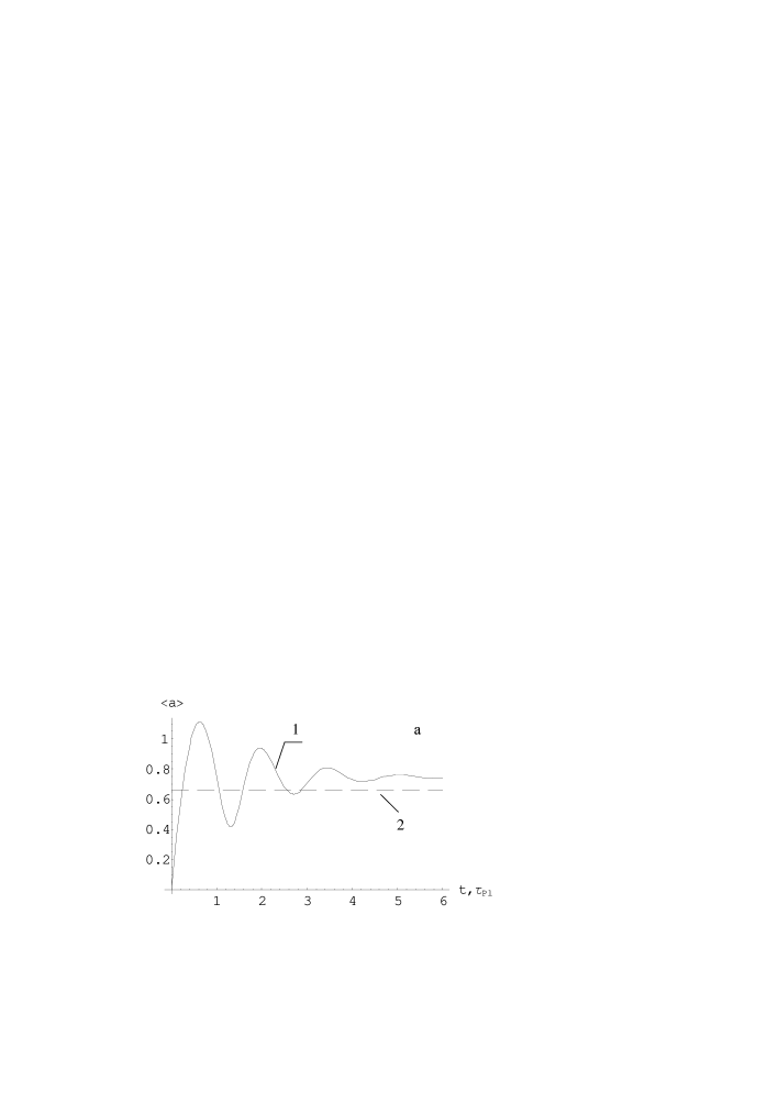
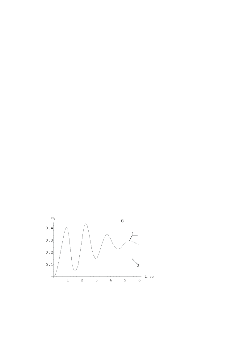
Figure 1: Evolution of the mean value of the scale factor (a) and its dispersion (b) calculated in the quasi-Heisenberg picture — (1). Dashed line (2) corresponds to the fully static picture when the Shrödinger norm of the wave function is used.

$$\ddot{\hat{a}}=-\frac{\dot{\hat{a}}^{2}}{2\hat{a}}-\frac{3\hat{{p}_{\phi}}^{2}}{2\hat{a}^{3}}-\frac{1}{2\hat{a}},$$

$$\dot{\hat{a}}=\frac{\hat{p_{a}}}{\hat{a}},~{}~{}~{}~{}~{}~{}\dot{\hat{\phi}}=\frac{\hat{p}_{\phi}}{\hat{a^{3}}},~{}~{}~{}~{}~{}\dot{\hat{p}_{\phi}}=0.$$ (14)

They have to be solved using the following operator initial conditions:

$$\hat{a}(0)=const=a,~{}~{}\hat{\phi}(0)=\phi,~{}~{}\hat{p}_{a}(0)=\frac{|\hat{p}_{\phi}|}{a},~{}~{}\hat{p}_{\phi}(0)=\hat{p}_{\phi},$$ (15)

where ${\hat{p}_{\phi}=-i\partial/\partial\phi}$. Thus, the initial values of operators satisfies the Hamiltonian constraint

$$-\frac{{\hat{p}}^{2}_{a}(0)}{2\hat{a}(0)}+\frac{{\hat{p}}^{2}_{\phi}(0)}{2{\hat{a}}^{3}(0)}+\frac{\hat{a}(0)}{2}=0.$$

The solution of the equations of motion is found in the momentum representation most easily. In this representation ${\hat{p}_{\phi}=k}$, ${\hat{\phi}=i\frac{\partial}{\partial k}}$. Finally, if one sets ${\hat{a}(0)=const=0}$, the solution of the equations of motion (14) are

$$a(\eta,k)=\sqrt{k}\sqrt[4]{\frac{1-\cos(4\eta)}{2}},$$ (16)

$$t(\eta,k)={2}^{-9/4}\sqrt{k}\int_{0}^{4\,\eta}\!\sqrt[4]{1-\cos(\xi)}{d\xi}.$$ (17)

in the parametric form.

The time-dependent quasi-Heisenberg operators act in a space of solutions of the Wheeler-DeWitt equation with the norm (12). In the momentum representation the formula for the average value of the operators [13, 14] looks like the ordinary quantum-mechanics one:

$$<A(t)>=\int\!{a}^{i|k|}c^{*}(k)A(k,a,t){a}^{-i|k|}{c}(k)\biggl{|}_{a\rightarrow 0}{dk}.$$ (18)

Using (16), (17), (18) one can calculate the average value of the scale factor of the Universe and its dispersion, for example, for the Universe state, which is described by the wave packet ${c(k)={k}^{2}{e^{-{k}^{2}}}}$. For this aim one has to solve Eqs. (16) and (17) numerically to find $a(k,t)$, and then substitutes it or its square to (18).

As it is shown in the Fig. 1, the average value of the scale factor decreases after expansion. But it does not turn to zero. The following oscillation has smaller amplitude and finally the evolution of the scale factor stops. This may be really interpreted as the time disappearance. It is interesting to note that the final static value is close to that from the static Shrödinger’s picture discussed in the beginning of the article (the same wave packet is used in the calculations).

Evolution of the Universe stops at the Planck times in our model. The expansion rate may increase if one takes a wave packet with a larger kinetic energy or a non-zero scalar field potential, which causes the inflation of Universe. According to Ref. [6] there are many Universes, in which the initial values of the scalar field have some distribution. Universes, in which the value of the scalar field is enough to produce the inflation, evolve like our Universe, while Universes, in which the value of the scalar field is low begin to collapse. Our paper describes namely such Universes, which come to the static state (that is to the disappearance of time) after the few oscillations.

To describe the real Universe, one must take to account the potential of the scalar field (it equals to zero in this paper). The solution of the operator equations of motion will be much more complicated. After all, the fundamental problem remains. According to Ref. [13], at some time the process of self-measurement takes a place. In this process the value of the scale factor is projected to different values at the different areas of space. The further evolution of these areas is classical. The modern Universe represents one of these areas. The problem is that the homogeneous model is insufficient to describe the process of self-measurement.

It should be noted that a time arrow appears in the quasi-Heisenberg picture of the closed Universe (see also discussion in Ref. [15]). This arrow has a direction to the end of the Universe evolution, i.e. to the static world appearance. The arrow of time results from the unification of gravity and quantum mechanics. There is no arrow of time in the evolution of the classical closed Universe, because the oscillations are symmetric relatively to the inversion of time. There is no arrow of time in quantum mechanics either, because it does not change after the inversion and complex conjugation of the Shrödinger equation.

[1] M. Kaku, Introduction to superstrings, Berlin: Springer-Verlag, 1988.

[2] J. A. Wheeler 1968 in: Battelle Recontres eds. B. DeWitt and J. A. Wheeler New York, 1968,p.

[3] B. S.DeWitt // Phys. Rev. 1967. Vol. 160. P. 1113.

[4] A. Mostafazadeh // Annals Phys. 2004. Vol. 309 P.1; arXiv: gr-qc/0306003.

[5] E. Guendelman and A. Kaganovich // Int. J.Mod. Phys. 1993. Vol. D 2. P. 221 (1993); arXiv: gr-qc/0302063.

[6] A.D. Linde. Particle physics and inflationary cosmology. Harwood academic press, Switzerland (1990).

[7] A. Vilenkin, Phys. Rev. D 39, 1116 (1989).

[8] B. L. Altshuler and A. O. Barvinsky // Uspekhi. Fiz. Nauk 1996 Vol. 166 P.459 [Sov. Phys. Usp. Vol. 39 P. 429] [10] A. Vilenkin //Phys. Rev. 1989. V. 39, P. 1116.

[9] C. J. Isham, arXiv: gr-qc/9210011;

[10] T. P. Shestakova and C. Simeone// Grav. Cosmol. 2004, Vol. 10 P. 161.; Ibid. Vol.10 P. 257.

[11] L.D.Landau, E.M.Lifshitz, The classical Theory of Fields, Oxford, Pergamon Press, 1982.

[12] A.D. Polyanin. Handbook of exact solutions for ordianary differential equations. New York, CRC Press,2000.

[13] S.L. Cherkas, V.L. Kalashnikov, preprint. arXiv:gr-qc/0512107.

[14] S.L. Cherkas, V.L. Kalashnikov// Grav. Cosmol. 2006. V.12 P. 126.

[15] C. Kiefer, H.D. Zeh//Phys. Rev. D 1995. V. 51, P. 4145.