$T\rightarrow 0$ mean-field population dynamics approach for the random $3$-satisfiability problem

Abstract

During the past decade, phase-transition phenomena in the random $3$-satisfiability ($3$-SAT) problem has been intensively studied by statistical physics methods. In this work, we study the random $3$-SAT problem by the mean-field first-step replica-symmetry-broken cavity theory at the limit of temperature $T\rightarrow 0$. The reweighting parameter $y$ of the cavity theory is allowed to approach infinity together with the inverse temperature $\beta$ with fixed ratio $r=y/\beta$. Focusing on the the system’s space of satisfiable configurations, we carry out extensive population dynamics simulations using the technique of importance sampling and we obtain the entropy density $s(r)$ and complexity $\Sigma(r)$ of zero-energy clusters at different $r$ values. We demonstrate that the population dynamics may reach different fixed points with different types of initial conditions. By knowing the trends of $s(r)$ and $\Sigma(r)$ with $r$, we can judge whether a certain type of initial condition is appropriate at a given $r$ value. This work complements and confirms the results of several other very recent theoretical studies.

I Introduction

Critical behaviors in the random $3$-satisfiability ($3$-SAT) problem were first reported by Kirkpatrick and Selman in 1994 Kirkpatrick and Selman (1994). Since then, physicists working in the field of spin glasses have done a lot of work on this important model system in theoretical computer science Monasson and Zecchina (1996, 1997). Mean-field calculations were done to understand the nature of the satisfiability (SAT-UNSAT) transition Monasson and Zecchina (1996, 1997); Monasson et al. (1999); Zhou (2005), to locate the SAT-UNSAT transition point Mézard et al. (2002); Mézard and Zecchina (2002); Mertens et al. (2006), and to analyze the performances of various algorithms Cocco and Monasson (2001). Based on the first-step replica-symmetry-broken (1RSB) mean-field cavity theory of spin glasses Mézard and Parisi (2001), Mézard, Parisi, and Zecchina created a powerful message-passing algorithm, namely survey propagation (SP), to find satisfiable solutions to random $3$-SAT formulas Mézard et al. (2002). The physical picture underlying the SP algorithm is that, when the density of constraints $\alpha$ of the system is close to the satisfiability threshold $\alpha_{\rm s}$, the solution space of a random $3$-SAT formula divides into many well-separated clusters. Mézard and co-workers also predicted that the SAT-UNSAT transition for the random $3$-SAT problem occurs at $\alpha_{\rm s}=4.2667$ Mézard and Zecchina (2002); Mertens et al. (2006). This threshold value lies within the rigorously known lower-bound $3.52$ Hajiaghayi and Sorkin (2003) and upper-bound $4.506$ Dubois et al. (2000) for random $3$-SAT, and the mean-field cavity SP solution is locally stable Montanari et al. (2004); Mertens et al. (2006); Zhou et al. (2007). The predicted SAT-UNSAT transition point of $\alpha_{\rm s}=4.2667$ is therefore conjectured to be exact.

The message-passing SP algorithm corresponds to the temperature $T=0$ (i.e., $\beta=1/T=+\infty$) limit of the 1RSB mean-field cavity theory of finite-connectivity spin glasses Mézard and Parisi (2001, 2003). This 1RSB cavity theory has an adjustable reweighting parameter $y$. In Refs. Mézard et al. (2002); Mézard and Zecchina (2002); Mertens et al. (2006), first the inverse temperature $\beta$ is set to infinity, and then $y$ is set to infinity. This means that the ratio $\lim_{T\rightarrow 0}y/\beta$ is equal to zero. On the other hand, it is now recognized that, to correctly characterize the equilibrium properties (as represented by the free-energy Gibbs measure) of a spin glass system, the reweighting parameter $y$ is required to take an appropriate value that is dependent on $\beta$. For a spin glass system with many-body interactions, there may exist a temperature range $T_{\rm d}\geq T\geq T_{\rm c}$ within which the optimal value of the reweighting parameter $y$ is equal to $\beta$ Kirkpatrick and Thirumalai (1987); Monasson (1995); Zhou and Li (2008). In the literature on structural glasses Kirkpatrick and Thirumalai (1987), $T_{\rm d}$ and $T_{\rm c}$ are referred to as the dynamical and static transition temperature of the system, respectively. For the random $3$-SAT problem with density of constraints $\alpha$, if the corresponding static transition temperature is located at $T_{\rm c}(\alpha)=0$, then the reweighting parameter $y$ and the inverse temperature $\beta$ should approach infinity with the same rate. In the present work, we investigate how the mean-field predictions on the ground-state properties of the random $3$-SAT problem depend on the ratio $y/\beta$. We generalize the cavity treatment of Refs. Mézard et al. (2002); Mézard and Zecchina (2002); Mertens et al. (2006) and study the statistical mechanics properties of the random $3$-SAT problem in the limit $\beta\rightarrow+\infty$ and $y\rightarrow+\infty$, with fixed ratio Mézard et al. (2005a)

$$r\equiv\frac{y}{\beta}\ .$$ (1)

Population dynamics simulations were performed based on a set of mean-field 1RSB cavity equations, and for each value of $\alpha$, the entropy density $s(r)$ and complexity $\Sigma(r)$ of the system as a function of the ratio $r$ are estimated. The entropy density $s(r)$ is a measure of the number of ground-energy configurations within one cluster of the configuration space, while the complexity $\Sigma(r)$ is a measure of the total number of such ground-energy clusters.

As the population dynamics simulations of this work were running, we noticed that questions closely related to the issue we discuss here were investigated earlier in Ref. Mézard et al. (2005a) in the context of the random $3$-coloring problem and more recently in Refs. Krzakala et al. (2007); Zdeborova and Krzakala (2007) for random $q$-coloring and random $K$-SAT. While the main focus of Ref. Krzakala et al. (2007) was on the limiting case of $r=1$, at which the numerical complexity of the mean-field theory can be reduced to some extent, detailed discussions on general values of $0\leq r\leq 1$ were presented in Refs. Zdeborova and Krzakala (2007); Montanari et al. (2008). The present paper confirms the physical picture given by Krzakala, Montanari, and co-workers Krzakala et al. (2007); Zdeborova and Krzakala (2007); Montanari et al. (2008) on the solution space structure of random $3$-SAT; it is complementary to these theoretical studies in three important ways. First, we introduce a different scheme of population dynamics with importance sampling (this scheme can be readily extended to finite temperatures); the numerical results obtained from this scheme are in agreement with those reported in Ref. Montanari et al. (2008). Second, we demonstrate that the population dynamics may reach different fixed points from different initial conditions. Third, we find that different initial conditions will lead to the same prediction on the properties of the dominating solution clusters of random $3$-SAT. This last point is rather interesting and needs to be further studied.

The main results of this paper are summarized here. When using the $F$-type initial condition as described in Sec. II.3, the population dynamics demonstrates that (i) at $\alpha=\alpha_{s}=4.2667$, $\Sigma(r)$ decreases monotonically with $r$ according to $\Sigma(r)=-0.020r^{2}$ and $s(r)$ increases monotonically with $r$; (ii) at $\alpha=4.2$, the complexity changes with $r$ following $\Sigma(r)=0.0059-0.023r^{2}$ and $s(r)$ still increases monotonically with $r$; (iii) at $\alpha=4.0$, both $\Sigma(r)$ and $s(r)$ have a discontinuity at $r=0$. When using the $U$-type initial condition of Sec. II.3, we find that both $\Sigma(r)$ and $s(r)$ are not monotonic functions of $r$. At the value of $r=1$, the complexity $\Sigma(1)$ and entropy density $s(1)$ as a function of the constraint density $\alpha$ are also calculated by population dynamics simulations with both the $F$-type and the $U$-type initial condition. The numerical data are consistent with the conclusion of Ref. Krzakala et al. (2007) that, for $\alpha<3.87$ the solution space of the random $3$-SAT problem forms a single cluster, while for $3.87\leq\alpha<\alpha_{\rm s}$ the solution space, although being nonergodic, is dominated by only a few (of order unity) solution clusters.

The paper is organized asfollows. Section II describes the mean-field cavity approach and the protocol of population dynamics simulations. The simulation results are reported and analyzed in Sec. III. We conclude our work in Sec. IV and discuss possible future extensions.

II Method

II.1 The factor-graph representation of the random $3$-SAT problem

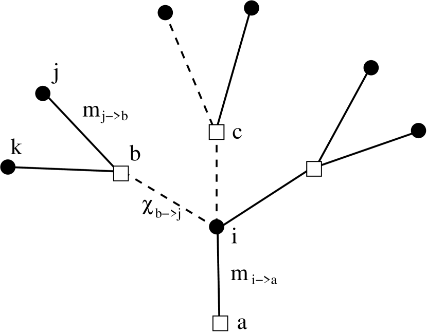
Figure 1: The factor-graph representation Kschischang et al. (2001); Mézard et al. (2002); Mézard and Zecchina (2002) for a random $3$-SAT formula. $m_{j\rightarrow b}$, $m_{i\rightarrow a}$ and $\chi_{b\rightarrow i}$ are messages on the edges of the factor-graph (explained in the main text).

A $3$-SAT formula contains $N$ Boolean variables and $M$ constraints, each of which involves $K=3$ variables. The degree of constrainedness of a random $3$-SAT formula is characterized by the constraint density $\alpha\equiv M/N$. A $3$-SAT formula can be represented by a factor graph ${\cal G}$ (see Fig. 1) of $N$ variable nodes (circles $i,j,k,\ldots$) and $M$ function nodes (squares $a,b,c,\ldots$) Kschischang et al. (2001); Mézard et al. (2002); Mézard and Zecchina (2002). Each function node $a$ corresponds to a constraint; it is connected to $K$ ($=3$) variable nodes $i\in\partial a$ (where $\partial a$ denotes the set of nearest neighbors of node $a$). Associated with each function node $a$ is an energy $E_{a}\in\{0,2\}$ of the form

$$E_{a}=2\prod\limits_{i\in\partial a}\frac{1-J_{a}^{i}\sigma_{i}}{2}\ .$$ (2)

In Eq. (2), $\sigma_{i}=\pm 1$ is the spin value of variable node $i$; $J_{a}^{i}=\pm 1$ is the coupling between node $i$ and node $a$. In the factor graph, the edge $(i,a)$ is a solid line if $J_{a}^{i}=1$ and it is a dashed line if $J_{a}^{i}=-1$. For a given $3$-SAT formula, the factor graph (with all its coupling constants) is fixed, while the spin configuration ${\bf\sigma}\equiv\{\sigma_{1},\sigma_{2},\ldots,\sigma_{N}\}$ can change. The total energy $E({\bf\sigma})$ of a given spin configuration is

$$E({\bf\sigma})=\sum\limits_{a\in{\cal G}}E_{a}\ .$$ (3)

A variable node $i$ of the factor graph ${\cal G}$ is connected to $k_{i}$ function nodes $a\in\partial i$. the vertex degree $k_{i}$ may be different for different variable nodes. For a random $3$-SAT formula with $N\gg 1$, the distribution of $k_{i}$ is governed by the Poisson distribution of mean $3\alpha$, i.e., ${\rm Prob}(k_{i}=k)=f_{3\alpha}(k)\equiv(3\alpha)^{k}e^{-3\alpha}/k!$. One can also define the $``$cavity degree” $k_{i\rightarrow a}$ of a variable node $i$ with respect to an edge $(a,i)$ as $k_{i\rightarrow a}\equiv|\partial i\backslash a|$. $k_{i\rightarrow a}$ is the number of nearest neighbors of node $i$ when edge $(a,i)$ is not considered. Obviously, $k_{i\rightarrow a}=k_{i}-1$. A useful property of random graphs is that the distribution of $k_{i\rightarrow a}$ is also governed by the Poisson distribution of mean $3\alpha$. We will use this property in the mean-field population dynamics simulations as described in Sec. II.3.

II.2 The cavity equations at a general low temperature $T$

At a sufficiently low temperature $T$, ergodicity of the whole configurational space $\Lambda$ of the model Eq. (3) breaks down. It is then assumed in mean-field theories Mézard and Parisi (2001); Mézard et al. (2002); Mézard and Zecchina (2002) that $\Lambda$ is split into an exponential number of ergodic subspaces. Each of these subspaces $\Lambda_{\alpha}$ corresponds to a macroscopic state (macrostate $\alpha$) of the system at temperature $T$. Based on the cavity approach of spin glasses Mézard and Parisi (2001); Mézard et al. (1987), the mean grand free-energy density of the random $3$-SAT problem can be derived. As the derivation details are well documented in the literature Mézard and Parisi (2001); Mézard and Zecchina (2002) (see also Refs. Zhou (2007); Zhou and Li (2008)), we shall directly list the final expressions and give only brief explanations.

At the 1RSB level of approximation, the total grand free energy of the random $K$-SAT system is

$$G_{\cal G}(\beta;y)=\sum\limits_{i\in{\cal G}}\Delta G_{i}-(K-1)\sum\limits_{a\in{\cal G}}\Delta G_{a}\ ,$$ (4)

where $\Delta G_{i}$ and $\Delta G_{a}$ are, respectively, the grand free-energy increase caused by adding variable node $i$ and function node $a$, with

$$\Delta G_{i}=-\frac{1}{y}\log\biggl{[}\prod\limits_{b\in\partial i}\bigl{(}\int{\rm d}{\chi}_{b\rightarrow i}\hat{P}_{b\rightarrow i}({\chi}_{b\rightarrow i})\bigr{)}\exp(-y\Delta F_{i})\biggr{]}$$ (5)

and

$$\Delta G_{a}=-\frac{1}{y}\log\biggl{[}\prod\limits_{j\in\partial a}\bigl{(}\int{\rm d}m_{j\rightarrow a}P_{j\rightarrow a}(m_{j\rightarrow a})\bigr{)}\exp(-y\Delta F_{a})\biggr{]}\ .$$ (6)

In Eqs. (5) and (6), $m_{i\rightarrow a}$ (the cavity magnetization) is the mean magnetization of vertex $i$ within one macrostate $\alpha$ when the edge $(a,i)$ is discarded, and $P_{i\rightarrow a}(m_{i\rightarrow a})$ is the distribution of this cavity magnetization among all the macrostates of the system. Similarly, $\chi_{b\rightarrow i}\equiv\prod_{j\in\partial b\backslash i}[(1-J_{b}^{j}m_{j\rightarrow b})/2]$ is the directed message from function node $b$ to variable node $i$ in one macrostate, and $\hat{P}_{b\rightarrow i}({\chi}_{b\rightarrow i})$ is the distribution of this message among all the macrostates. $\Delta F_{i}$ and $\Delta F_{a}$ are, respectively, the free-energy increase of macrostate $\alpha$ due to the addition of variable node $i$ and function node $a$, with

$$\Delta F_{i} = -\frac{1}{\beta}\log\biggl{[}{\prod\limits_{b\in\partial i}^{(-)}}\bigl{[}1-(1-e^{-2\beta}){\chi}_{b\rightarrow i}\bigr{]}$$ (7)

$$+{\prod\limits_{b\in\partial i}^{(+)}}\bigl{[}1-(1-e^{-2\beta}){\chi}_{b\rightarrow i}\bigr{]}\biggr{]}\ ,$$

$$\Delta F_{a} = -\frac{1}{\beta}\log\biggl{[}1-(1-e^{-2\beta})\prod\limits_{j\in\partial a}\frac{(1-J_{a}^{j}m_{j\rightarrow a})}{2}\biggr{]}\ .$$ (8)

In Eq. (7), the $\prod\limits^{(-)}$ and $\prod\limits^{(+)}$ indicate that the multiplication is restricted to the neighbors $b$ of $i$ for which $J_{b}^{i}=-1$ and $J_{b}^{i}=+1$, respectively.

On each edge $(a,i)$ of factor graph ${\cal G}$, the probability distributions $P_{i\rightarrow a}$ and $\hat{P}_{a\rightarrow i}$ are required to satisfy the variational condition that

$$\frac{\delta G_{{\cal G}}(\beta;y)}{\delta P_{i\rightarrow a}}=\frac{\delta G_{{\cal G}}(\beta;y)}{\delta\hat{P}_{a\rightarrow i}}\equiv 0\ .$$ (9)

This variational condition is satisfied by the following two self-consistent equations on each directed edge $a\rightarrow i$ and $i\rightarrow a$:

$$\hat{P}_{a\rightarrow i}({\chi}_{a\rightarrow i})=\prod\limits_{j\in\partial a\backslash i}\bigl{[}\int{\rm d}m_{j\rightarrow a}P_{j\rightarrow a}(m_{j\rightarrow a})\bigr{]}\delta\biggl{(}\chi_{a\rightarrow i}-\prod\limits_{j\in\partial a\backslash i}\frac{(1-J_{a}^{j}m_{j\rightarrow a})}{2}\biggr{)}$$ (10)

and

$$P_{i\rightarrow a}(m_{i\rightarrow a})=\frac{\prod\limits_{b\in\partial i\backslash a}\bigl{[}\int{\rm d}\chi_{b\rightarrow i}\hat{P}_{b\rightarrow i}(\chi_{b\rightarrow i})\bigr{]}e^{-y\Delta F_{i\rightarrow a}}\delta\bigl{(}m_{i\rightarrow a}-M(\{\chi_{b\rightarrow i}:b\in\partial i\backslash a\}\bigr{)}}{\prod\limits_{b\in\partial i\backslash a}\bigl{[}\int{\rm d}\chi_{b\rightarrow i}\hat{P}_{b\rightarrow i}(\chi_{b\rightarrow i})\bigr{]}e^{-y\Delta F_{i\rightarrow a}}}\ ,$$ (11)

with $M(\{{\chi}_{b\rightarrow i}:b\in\partial i\backslash a\})$ being the shorthand notation for

$$M(\{\chi_{b\rightarrow i}:b\in\partial i\backslash a\})\equiv\frac{{\prod\limits_{b\in\partial i\backslash a}^{(-)}}\bigl{[}1-(1-e^{-2\beta})\chi_{b\rightarrow i}\bigr{]}-{\prod\limits_{b\in\partial i\backslash a}^{(+)}}\bigl{[}1-(1-e^{-2\beta})\chi_{b\rightarrow i}\bigr{]}}{{\prod\limits_{b\in\partial i\backslash a}^{(-)}}\bigl{[}1-(1-e^{-2\beta})\chi_{b\rightarrow i}\bigr{]}+{\prod\limits_{b\in\partial i\backslash a}^{(+)}}\bigl{[}1-(1-e^{-2\beta})\chi_{b\rightarrow i}\bigr{]}}\ .$$ (12)

The free-energy increase $\Delta F_{i\rightarrow a}$ in Eq. (11) is calculated by Eq. (7) but with $b\in\partial i$ being replaced by $b\in\partial i\backslash a$ [i.e., discarding the effect of edge $(i,a)$].

II.3 The $T\rightarrow 0$ limit and population dynamics simulations

Let us now consider the zero-temperature limit (i.e., $\beta\rightarrow+\infty$) of the cavity equations of the preceding subsection. We focus on the SAT phase of the random $3$-SAT problem and assume the Hamiltonian Eq. (3) has at least one zero-energy ground state. In the SAT phase at the $\beta\rightarrow+\infty$ limit, the free energy of each macrostate is completely contributed by entropy.

For the benefit of later discussions, let us introduce two further shorthand notations $Z_{i}$ and $Z_{a}$,

$$Z_{i} \equiv {\prod\limits_{b\in\partial i}^{(-)}}\bigl{(}1-{\chi}_{b\rightarrow i}\bigr{)}+{\prod\limits_{b\in\partial i}^{(+)}}\bigl{(}1-{\chi}_{b\rightarrow i}\bigr{)}\ ,$$ (13)

$$Z_{a} \equiv 1-\prod\limits_{j\in\partial a}\frac{(1-J_{a}^{j}m_{j\rightarrow a})}{2}\ .$$ (14)

Then at $\beta\rightarrow\infty$ and fixed ratio $r$, the grand free-energy increases $\Delta G_{i}$ and $\Delta G_{a}$ can be reexpressed as

$$y\Delta G_{i} = -\log\Bigl{[}\prod\limits_{b\in\partial i}\bigl{(}\int{\rm d}{\chi}_{b\rightarrow i}\hat{P}_{b\rightarrow i}({\chi}_{b\rightarrow i})\bigr{)}\Theta(Z_{i})e^{r\log(Z_{i})}\Bigr{]}\ ,$$ (15)

$$y\Delta G_{a} = -\log\Bigl{[}\prod\limits_{i\in\partial a}\bigl{(}\int{\rm d}{m}_{i\rightarrow a}P_{i\rightarrow a}({m}_{i\rightarrow a})\bigr{)}\Theta(Z_{a})e^{r\log(Z_{a})}\Bigr{]}\ .$$ (16)

In Eqs. (5) and (6), $\Theta(x)=1$ if $x>0$ and $\Theta(x)=0$ if $x\leq 0$.

In the thermodynamic limit of graph size $N\rightarrow\infty$ and $M\rightarrow\infty$ (with $\alpha$ being finite), the grand free-energy density $g(r)$ of the random $3$-SAT system is expressed as

$$yg(r)=y\overline{\Delta G_{i}}-2\alpha y\overline{\Delta G_{a}}\ ,$$ (17)

where the overlines indicate averaging over all the possible local environments of the involved variable node $i$ or function node $a$. The complexity $\Sigma(r)$ and mean entropy density $s(r)$ of the system are related to $g(\beta;y)$ by (see, e.g., Ref. Zhou and Li (2008))

$$\Sigma(r) = -yg(r)+r\Bigl{(}\overline{\langle\beta\Delta F_{i}\rangle}-2\alpha\overline{\langle\beta\Delta F_{a}\rangle}\Bigr{)}\ ,$$ (18)

$$s(r) = -\Bigl{(}\overline{\langle\beta\Delta F_{i}\rangle}-2\alpha\overline{\langle\beta\Delta F_{a}\rangle}\Bigr{)}\ .$$ (19)

The mean free-energy increase of $\Delta F_{i}$ and $\Delta F_{a}$ as averaged over all the macrostate of the system is calculated through

$$\langle\beta\Delta F_{i}\rangle = -\frac{\prod\limits_{b\in\partial i}\bigl{[}\int{\rm d}{\chi}_{b\rightarrow i}\hat{P}_{b\rightarrow i}({\chi}_{b\rightarrow i})\bigr{]}\Theta(Z_{i})e^{r\log(Z_{i})}\log(Z_{i})}{\prod\limits_{b\in\partial i}\bigl{[}\int{\rm d}{\chi}_{b\rightarrow i}\hat{P}_{b\rightarrow i}({\chi}_{b\rightarrow i})\bigr{]}\Theta(Z_{i})e^{r\log(Z_{i})}}\ ,$$ (20)

$$\langle\beta\Delta F_{a}\rangle = -\frac{\prod\limits_{i\in\partial a}\bigl{[}\int{\rm d}{m}_{i\rightarrow a}{P}_{i\rightarrow a}({m}_{i\rightarrow a})\bigr{]}\Theta(Z_{a})e^{r\log(Z_{a})}\log(Z_{a})}{\prod\limits_{i\in\partial a}\bigl{[}\int{\rm d}{m}_{i\rightarrow a}{P}_{i\rightarrow a}({m}_{i\rightarrow a})\bigr{]}\Theta(Z_{a})e^{r\log(Z_{a})}}\ .$$ (21)

At a given value of constraint density $\alpha$, we use population dynamics Mézard and Parisi (2001) to calculate the complexity $\Sigma(r)$ and entropy density $s(r)$ for the random $3$-SAT problem. The iterative equation (11) for the cavity magnetization distributions $P_{i\rightarrow a}(m_{i\rightarrow a})$ are implemented according to the following protocol of importance sampling.

(1)

. A total number of ${\cal N}$ sets are stored in the computer memory. Each set, which represents a probability distribution $P_{i\rightarrow a}(m_{i\rightarrow a})$ of a cavity magnetization, contains ${\cal M}$ double-precision values $-1\leq m_{i\rightarrow a}\leq 1$. These ${\cal N}$ sets are independently initialized according to a certain type of initial condition (see below).

(2)

. To perform a single update to the stored population of distributions, the follow steps occur:

(i)

A random integer $n$ is generated according to the Poisson distribution $f_{3\alpha}(n)$.

(ii)

$2n$ sets (denoted by $P_{j_{1}\rightarrow b_{1}},P_{k_{1}\rightarrow b_{1}},\ldots,P_{j_{n}\rightarrow b_{n}},P_{k_{n}\rightarrow b_{n}}$) are randomly chosen with replacement from the stored ${\cal N}$ sets, and $3n$ coupling constants $\{J_{b_{l}}^{j_{l}},J_{b_{l}}^{k_{l}},J_{b_{l}}^{i}\}$ are generated, each of which is independently assigned a value $+1$ or $-1$ with probability one-half.

(iii)

$2n$ cavity magnetizations $(m_{j_{1}\rightarrow b_{1}},m_{k_{1}\rightarrow b_{1}})$, $\ldots$, $(m_{j_{n}\rightarrow b_{n}},m_{k_{n}\rightarrow b_{n}})$ are sampled uniformly from these $2n$ sets, respectively, and $n$ values $\chi_{b_{l}\rightarrow i}=[(1-J_{b_{l}}^{j_{l}}m_{j_{l}\rightarrow b_{l}})(1-J_{b_{l}}^{k_{l}}m_{k_{l}\rightarrow b_{l}})/4$ are calculated.

(iv)

$Z_{i}=\prod_{b_{l}:J_{b_{l}}^{i}=-1}(1-{\chi}_{b_{l}\rightarrow i})+\prod_{b_{l}:J_{b_{l}}^{i}=+1}(1-{\chi}_{b_{l}\rightarrow i})$ is calculated and a new cavity magnetization $m_{i\rightarrow a}=[\prod_{b_{l}:J_{b_{l}}^{i}=-1}(1-{\chi}_{b_{l}\rightarrow i})-\prod_{b_{l}:J_{b_{l}}^{i}=+1}(1-{\chi}_{b_{l}\rightarrow i})]/Z_{i}$ is calculated.

(v)

This new $m_{i\rightarrow a}$ value is accepted with probability proportional to $\Theta(Z_{i})\exp[r\log(Z_{i})]$ by way of the Metropolis importance-sampling method Newman and Barkema (1999) and, if it is rejected, the old $m_{i\rightarrow a}$ value is retained.

(vi)

Repeat (iii)–(v) a number of ${\cal M}\times{\cal L}$ times and generate a new set $P_{i\rightarrow a}$ with ${\cal M}$ independent $m_{i\rightarrow a}$ values (sampled with interval ${\cal L}$). Obtain the value of $y\Delta G_{i}$ and $\langle\beta\Delta F_{i}\rangle$ as expressed by Eqs. (15) and (20) using the sampled data of these ${\cal M}\times{\cal L}$ repeats.

(vii)

Replace a randomly chosen stored old set with the newly generated set $P_{i\rightarrow a}$.

(3)

. Repeat step (${\bf 2}$) three times to obtain three probability distributions $P_{i\rightarrow a}(m_{i\rightarrow a})$, $P_{j\rightarrow a}(m_{j\rightarrow a})$, and $P_{k\rightarrow a}(m_{k\rightarrow a})$. A total number of ${\cal M}\times{\cal L}$ triples $(m_{i\rightarrow a},m_{j\rightarrow a},m_{k\rightarrow a})$ are then sampled uniformly. From these sampled data, $y\Delta G_{a}$ and $\langle\beta\Delta F_{a}\rangle$ as expressed by Eqs. (16) and (21) are calculated.

(4)

. Repeat steps (${\bf 2}$) and (${\bf 3}$) a number ${\cal T}_{1}\times{\cal N}$ of times for the population dynamics to reach a steady state and another number ${\cal T}_{2}\times{\cal N}$ of times to collect values of $y\Delta G_{i}$, $y\Delta G_{a}$, $\langle\beta\Delta F_{i}\rangle$, and $\langle\beta\Delta F_{a}\rangle$. From these collected values, the grand free-energy density $g(r)$, the complexity $\Sigma(r)$, and the mean entropy density $s(r)$ are calculated according to Eqs. (17), (18), and (19), respectively. The standard deviations of the numerical results are estimated by the bootstrap method Efron (1979).

The above-mentioned population dynamics procedure is quite time-consuming. The total simulation time is roughly proportional to ${\cal N}{\cal M}{\cal L}({\cal T}_{1}+{\cal T}_{2})$. We have used different sets of parameter values to reach a balance between high numerical precision and computation time. The data reported in the next section are obtained with the following set of parameters: ${\cal N}=1000$, ${\cal M}=2000$, ${\cal L}=50$, ${\cal T}_{1}=500$, and ${\cal T}_{2}=1500$ (with the exception that, in Fig. 5, the simulation results at $\alpha=3.875$ and $3.9$, which are close to the ergodicity transition point of the random $3$-SAT system, are obtained with ${\cal N}=2016$ and ${\cal L}=100$). At each pair of values $(\alpha,r)$, this set of parameters leads to satisfactory numerical precision with a tolerable simulation time of about ten days (through a present-day personal computer). If we use ${\cal N}=2000$ and ${\cal M}=4000$ in the simulation, the mean values of the calculated thermodynamic densities will not change much, while their standard deviations can be reduced to about half the level of those reported in the next section.

It is recognized by test runs that the results of the population dynamics can have a strong dependence on initial condition. The set of self-consistent equations (10) and (11) for the random $3$-SAT problem may have more than one stable fixed point. To investigate this initial condition dependence, we use the following two major types of initial conditions to produce numerical data of the next section.

F-type.

The cavity magnetization distribution $P_{i\rightarrow a}(m_{i\rightarrow a})$ at the beginning of the population dynamics is set to be $P_{i\rightarrow a}(m_{i\rightarrow a})=0.45\ \delta(m_{i\rightarrow a},1)+0.45\ \delta(m_{i\rightarrow a},-1)+0.1\ u(m_{i\rightarrow a})$, where $u(x)$ is the uniform distribution over $-1<x<1$. This initial condition assumes that the spin value of a vertex $i$ is frozen in most of the macrostates.

U-type.

The initial cavity magnetization distribution $P_{i\rightarrow a}(m_{i\rightarrow a})$ is set to be $P_{i\rightarrow a}(m_{i\rightarrow a})=u(m_{i\rightarrow a})$ with $-1<m_{i\rightarrow a}<1$. This condition assumes that initially the spin value of a vertex is unfrozen in all the macrostates.

The plausibility of each of these two initial conditions will be judged by its predictions.

III Results

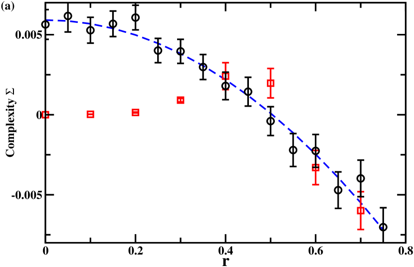
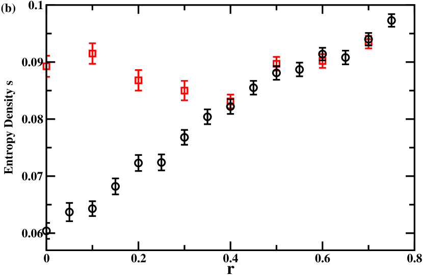
Figure 2: (Color Online) The complexity (a) and mean entropy density (b) for the random $3$-SAT problem with constraint density $\alpha=4.2$. Black circles and red square are, respectively, simulation results obtained using the $F$-type and the $U$-type initial condition. The blue dashed line in (a) is a fitting to the circular points with $\Sigma(r)=0.0059(2)-0.023(1)\ r^{2}$.

III.1 Population dynamics at $\alpha=4.2$

At $\alpha=4.2$, the complexity $\Sigma(r)$ and the mean entropy density $s(r)$ of the random $3$-SAT are shown in Fig. 2 for $0\leq r\leq 0.75$. Under the $F$-type initial condition, the obtained complexity values can be fitted by $\Sigma(r)=a-br^{2}$ with $a=0.0059\pm 0.0002$ and $b=0.023\pm 0.001$, while the mean entropy density $s(r)$ increases monotonically from $s(0)=0.060\pm 0.001$ to $s(0.75)=0.097\pm 0.001$. These results appear to be quite reasonable: (i) According to Refs. Kirkpatrick and Thirumalai (1987); Monasson (1995); Zhou and Li (2008), as $r$ increases, the complexity should decrease and the mean entropy density should increase; (ii) the value of $\Sigma(0)$ agrees with the prediction of the SP algorithm Mézard and Zecchina (2002), which gives $\Sigma(0)=0.00599$; (iii) $\Sigma(1)$ is negative, in agreement with Ref. Krzakala et al. (2007). The mean-field theory suggests that the solution space of a typical long random $3$-SAT formula with constraint density $\alpha=4.2$ is dominated by a few clusters of entropy density $s\approx s(0.5)=0.088\pm 0.001$ [with $\Sigma(0.5)\approx 0$], although clusters of lower entropy density $s=s(0)\approx 0.060$ are most abundant in the solution space. These two entropy density values are in agreement with the results of Ref. Montanari et al. (2008).

When $r\geq 0.4$, the complexity and mean entropy density values reported by the population dynamics with the $U$-type initial condition are in agreement with those obtained with the $F$-type initial condition. For $r\geq 0.4$, the mean-field population dynamics is insensitive to initial conditions. However, under the $U$-type initial condition the complexity $\Sigma(r)$ increases with $r$ and the mean entropy density $s(r)$ decreases with $r$ when $r\in[0,0.4)$. This behavior is unphysical, because the mean entropy density $s(r)$ should be an increasing function of $r$ Zhou and Li (2008). Therefore, under the $U$-type initial condition, the parameter $r$ should not be set to values lower than $0.4$. Under the $U$-type initial condition, the fixed point of the population dynamics at $r=0$ corresponds to the replica-symmetric solution of the SP algorithm Mézard and Zecchina (2002). This replica-symmetric solution is always stable in the mean-field theory of Ref. Mézard and Zecchina (2002), as entropic effects are completely neglected. When the entropy of each zero-energy macrostate is properly considered in the mean-field theory, the present paper indicates that this replica-symmetric solution is no longer stable (see also Refs. Krzakala et al. (2007); Montanari et al. (2008)). To get physically meaningful results for $0\leq r<0.4$ under the $U$-type initial condition, it is necessary to assume further organization of the solution space of the random $3$-SAT problem (splitting of a cluster of solutions into many subclusters of solutions). Implementing this higher-order hierarchical structure into the population dynamics is conceptually simple, but the algorithm will be extremely demanding on computer time and memory space.

III.2 Population dynamics at $\alpha=4.2667$

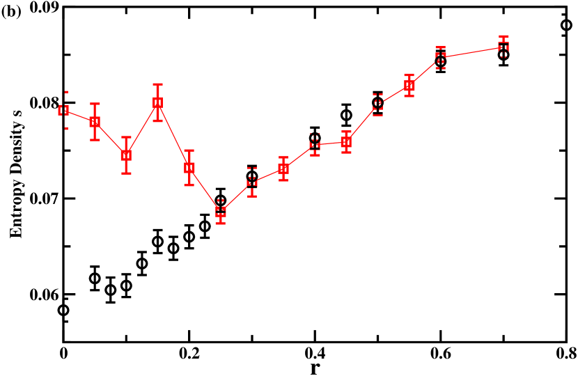
Figure 3: (Color Online) The complexity (a) and mean entropy density (b) for the random $3$-SAT problem with constraint density $\alpha=4.2667$. Black circles and red square are, respectively, simulation results obtained using the $F$-type and the $U$-type initial condition. The blue dashed line in (a) is a fitting to the circular points with $\Sigma(r)=-0.020(1)\ r^{2}$, while the black dotted line marks $\Sigma(r)\equiv 0$.

The SAT-UNSAT transition of the random $3$-SAT problem is predicted to occur at $\alpha=4.2667$ Mézard and Zecchina (2002); Mertens et al. (2006). At this density of constraints, Fig. 3 shows how the complexity and entropy density change with the ratio $r$. Under the $F$-type initial condition, the complexity decreases with $r$ according to $\Sigma(r)=-br^{2}$ with $b=0.020\pm 0.001$; and consistently, the entropy density $s(r)$ increases with $r$ monotonically. The present work, therefore, further confirms that the satisfiability transition of the random $3$-SAT takes place at $\alpha=4.2667$: including the entropic effect into the mean-field theory does not change the predicted location of the SAT-UNSAT transition. At this transition point, a typical random $3$-SAT formula of length $N$ still has an exponential number $\exp\bigl{[}Ns(0)\bigr{]}$ of satisfiable solutions, with $s(0)=0.058\pm 0.001$. But it is extremely difficult for a local or global algorithm to find one such solution.

As in the case of $\alpha=4.2$, if the $U$-type initial condition is applied, both the calculated complexity $\Sigma(r)$ and mean entropy density $s(r)$ do not change monotonically with $r$. Figure 3 indicates that the results from the $U$-type initial condition are valid only for $r\geq 0.25$. For $0\leq r\leq 0.2$, as the increasing trend of the complexity $\Sigma(r)$ and the decreasing trend of the entropy density $s(r)$ are not physically meaningful, the positivity of $\Sigma(r)$ cannot be taken as evidence that the random $3$-SAT is still in the SAT phase at $\alpha=4.2667$.

III.3 Population dynamics at $\alpha=4.0$

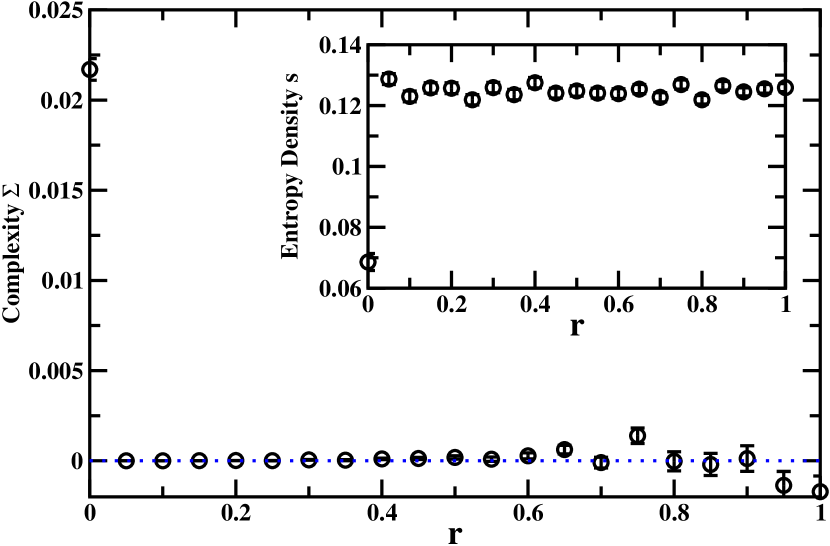
Figure 4: (Color Online) The complexity and mean entropy density (inset) for the random $3$-SAT problem with constraint density $\alpha=4.0$. Black circles are simulation results obtained using the $F$-type initial condition. The blue dashed line marks $\Sigma(r)\equiv 0$.

For $\alpha=4.2667$ and $4.2$, the complexity $\Sigma(r)$ calculated with the $F$-type initial condition reaches maximum at $r=0$ and it has the form $\Sigma(r)=a-br^{2}$ when $r\in[0,1)$. However, Fig. 4 demonstrates that a different situation occurs for $\alpha=4.0$. At this density of constraints, the population dynamics with $r=0$ and the $F$-type initial condition reports a complexity value $\Sigma(0)=0.0217\pm 0.0006$ (agreeing with the prediction of the SP algorithm Mézard and Zecchina (2002)) and a mean entropy density value $s(0)=0.069\pm 0.003$. But as the ratio $r$ is set to slightly positive values, the complexity suddenly drops to $\Sigma(r)\approx 0$ while the mean entropy density jumps to $s(r)\approx 0.125$. As $r$ increases further, both $\Sigma(r)$ and $s(r)$ keep almost constant until $r$ is close to unity. For $r\geq 0.8$, $\Sigma(r)$ and $s(r)$ have, respectively, a decreasing and an increasing trend. The discontinuity at $r=0$ for both $\Sigma(r)$ and $s(r)$ was totally unexpected (we have performed population dynamics simulations with different $F$-type initial conditions to rule out the possibility of numerical artifact). Similar discontinuity was also observed in the $q$-coloring problem Zdeborova and Krzakala (2007). If we look at the steady-state cavity magnetization distributions $P_{i\rightarrow a}(m_{i\rightarrow a})$, we find that they are far from being in the form of a $\delta$-function in the whole range of $0\leq r\leq 1$. This later observation confirms that at $\alpha=4.0$, the ergodicity property of the solution space of the random $3$-SAT is indeed violated. Figure 4 indicates that at $\alpha=4.0$, the solution space of the random $3$-SAT problem is organized far more complex than what has been assumed in the mean-field theory. This point should be investigated more thoroughly.

For the limiting case of $r=0$, it has already been shown that the mean-field solution at the first-step replica-symmetry-broken level is unstable toward the full-step replica-symmetry-broken level Montanari et al. (2004); Mertens et al. (2006) for $\alpha<4.153$. The different behaviors demonstrated in Figs. 2, 3, and 4 for $\alpha=4.2,4.2667$, and $4.0$ confirm the earlier stability analysis Montanari et al. (2004); Mertens et al. (2006) and further suggest that, if the 1RSB mean-field solution is unstable at $r=0$, it will be unstable when $r$ is positive but less than a certain threshold value $r_{\rm th}$. This threshold value may be smaller or larger than unity (for $\alpha=4.0$, it appears that $r_{\rm th}\approx 0.8$).

III.4 Population dynamics at $r=1$

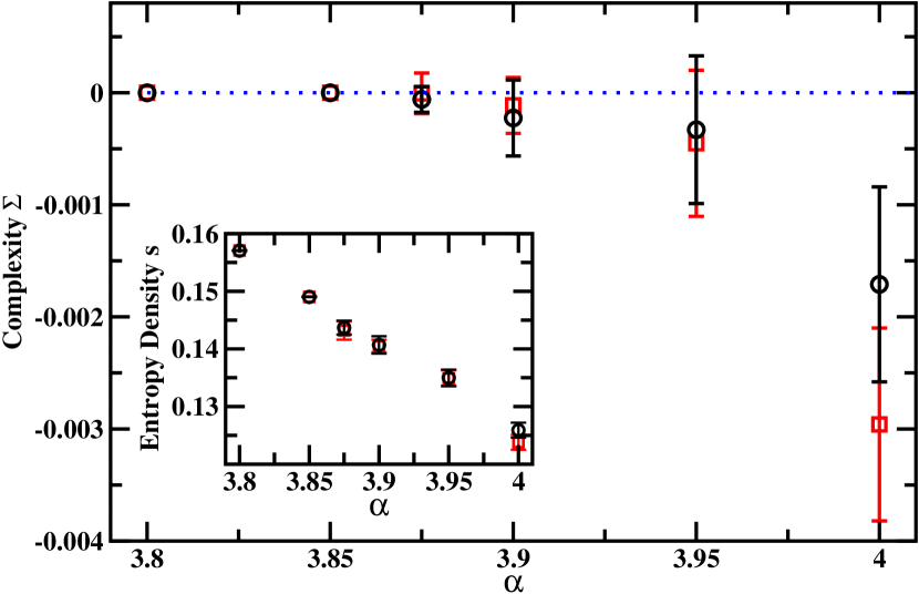
Figure 5: The complexity $\Sigma(r=1)$ and the mean entropy density $s(r=1)$ for the random $3$-SAT problem with constraint density $\alpha$. Black circles and red squares correspond to the $F$-type and the $U$-type initial condition, respectively. The blue dotted line marks $\Sigma\equiv 0$.

Now let us fix $r=1$ and study how the complexity $\Sigma(1)$ and mean entropy density $s(1)$ change with the constraint density $\alpha$. Using an elegant tree reconstruction technique, Montanari and co-authors Krzakala et al. (2007) found that, for the random $3$-SAT problem, $\Sigma(1)$ changes from being exactly zero to being negative at $\alpha\approx 3.87$. The alternative population dynamics approach of the present paper reports consistent results (see Fig. 5). For $\alpha=3.8$ and $3.85$, we have checked that the steady-state distributions $P_{i\rightarrow a}(m_{i\rightarrow a})$ of cavity magnetizations are all $\delta$-functions (ergodicity property of the solution space is not violated). For $\alpha\geq 3.875$, simulations with both the $F$-type and $U$-type initial condition give negative values for the complexity $\Sigma(1)$. At $\alpha$ very close to the ergodicity transition point of $3.87$, we have also observed that the population dynamics simulation needs a much longer time to reach steady state. This behaviors is very probably caused by the divergence of relaxation times of the population dynamics at the vicinity of the ergodicity transition ($\alpha\approx 3.87$). Such a critical slowing-down was investigated analytically and numerically in Ref. Weigt and Zhou (2006).

When $\alpha>3.87$, very probably most of the satisfying solutions of a random $3$-SAT formula can be grouped into one of a subexponential number of clusters of solutions Krzakala et al. (2007); Zhou and Li (2008). It will then be very difficult to prove mathematically the clustering of solutions following the method of Ref. Mézard et al. (2005a).

IV Conclusion and discussion

In this paper, we studied a spin glass model of the random $3$-SAT problem at the temperature $T\rightarrow 0$ limit by the mean-field first-step replica-symmetry-breaking (1RSB) cavity method. The reweighting parameter $y$ (corresponding to the level of macrostates) and the inverse temperature $\beta$ were allowed to approach infinity with fixed ratio $r=y/\beta$. The complexity and mean entropy density of the random $3$-SAT are calculated as a function of $r$ by population dynamics simulations. The sensitivity to initial conditions of the simulation results was investigated by initializing the cavity magnetization distributions in two different way (see Sec. II.3).

When the $F$-type initial condition is used, at $\alpha=4.2$ the complexity $\Sigma(r)$ decreases monotonically with $r$ and becomes negative when $r$ exceeds $0.5$; the mean entropy density $s(r)$ increases monotonically with $r$. The most abundant clusters of solutions of the random $3$-SAT system correspond to $r=0$ and have mean entropy density $s(0)\approx 0.060$, but the (few) dominating clusters of solutions correspond to $r\approx 0.5$ and have mean entropy density $s(0.5)\approx 0.088$. The complexity $\Sigma(r=0)$ decreases continuously with $\alpha$ and reaches zero at $\alpha=4.2667$, where the random $3$-SAT experiences a SAT-UNSAT transition. At this critical constraint density, the solution space of the random $3$-SAT still has a positive mean entropy density $s(0)\approx 0.058$.

When the $U$-type initial condition is applied, the complexity $\Sigma(r)$ and mean entropy density $s(r)$ are both nonmonotonic functions of $r$. At $\alpha=4.2$, the population dynamics algorithm reported a zero complexity value at $r=0$. As $r$ becomes positive, $\Sigma(r)$ first increases with $r$, reaches a maximal value at $r\approx 0.4$, and then decreases with $r$. The mean entropy density $s(r)$ has a reverse trend. The non-monotonic behaviors of $\Sigma(r)$ and $s(r)$ indicate that, for the $U$-type initial condition the population dynamics will not report physically meaningful results if $r$ is close to zero. At $\alpha=4.0$, if the parameter $r$ is set close to zero, even the population dynamics with the $F$-type initial condition will fail to get plausible results.

At $r=1$, the complexity and mean entropy density as a function of constraint density $\alpha$ were also investigated by population dynamics. For $\alpha=3.85$ or lower, ergodicity of the solution space of the random $3$-SAT is unbroken and the complexity is exactly zero. For $\alpha=3.875$ or higher, the population dynamics with both the $F$-type and the $U$-type initial condition predicted negative values for $\Sigma(1)$. The zero-energy configuration space of the random $3$-SAT problem clusters into many subspaces for $\alpha>3.875$, but only subexponential clusters are dominating the configuration space, in agreement with Ref. Krzakala et al. (2007).

This paper focused on the zero-energy configurational space of the random $3$-SAT problem. When the ground-state energy of the system becomes positive, the $T\rightarrow 0$ limit formulas in Sec. II.3 need to be revised. Most importantly, in a given macrostate a cavity magnetization $m_{i\rightarrow a}$ may take one of the following three possible forms:

$$m_{i\rightarrow a}=\left\{\begin{array}[]{l}1-m_{i\rightarrow a}^{+}e^{-2\beta}\\ \\ -1+m_{i\rightarrow a}^{-}e^{-2\beta}\\ \\ m_{i\rightarrow a}^{0}\end{array}\right.$$ (22)

where $-1<m_{i\rightarrow a}^{0}<1$, $m_{i\rightarrow a}^{+}\geq 0$, and $m_{i\rightarrow a}^{-}\geq 0$. In the present paper, we have simply set $m_{i\rightarrow a}^{+}=m_{i\rightarrow a}^{-}=0$ without affecting the results of population dynamics, but for systems with positive ground-state energies, the more general formula should be used. Even if the ground-state energy of the system is zero, Eq. (22) should be used if one wants to study the properties of metastable macrostates (with positive minimal energies) or the low-temperature properties of the system. We will return to this point in a later publication.

As Refs. Krzakala et al. (2007); Montanari et al. (2008) and the present paper demonstrate, the zero-energy configuration space of the random $3$-SAT problem is divided into clusters of different sizes. For the random $3$-SAT problem, will the minimal-energy configurations with a given positive energy value $E$ also be split into clusters of different entropies $S$? To detect such a possibility, a natural extension is to introduce two reweighting parameters (say $y$ and $r$) for both energy and entropy, and to reweight each minimal-energy cluster $\alpha$ by a factor $\exp(-yE+rS)$. Together with Krzakala and Zdeborova, we are working on this point for the random $3$-SAT problem and the $q$-coloring problem.

Although physicists believe that the solutions of a large random $3$-SAT formula are organized into well separated subspaces, clustering of random $K$-SAT solutions has been rigorously proven only for $K\geq 8$ Mézard et al. (2005b). Recently, there has been a lot of simulation work on this important issue (e.g., Ardelius et al. (2007); Ardelius and Zdeborová (2008)), but a lot of work still remains to be done to fully understand the energy landscape of the random $3$-SAT problem.

References

- Kirkpatrick and Selman (1994) S. Kirkpatrick and B. Selman, Science 264, 1297 (1994).
- Monasson and Zecchina (1996) R. Monasson and R. Zecchina, Phys. Rev. Lett. 76, 3881 (1996).
- Monasson and Zecchina (1997) R. Monasson and R. Zecchina, Phys. Rev. E 56, 1357 (1997).
- Monasson et al. (1999) R. Monasson, R. Zecchina, S. Kirkpatrick, B. Selman, and L. Troyansky, Nature 400, 133 (1999).
- Zhou (2005) H. Zhou, New J. Phys. 7, 123 (2005).
- Mézard et al. (2002) M. Mézard, G. Parisi, and R. Zecchina, Science 297, 812 (2002).
- Mézard and Zecchina (2002) M. Mézard and R. Zecchina, Phys. Rev. E 66, 056126 (2002).
- Mertens et al. (2006) S. Mertens, M. Mézard, and R. Zecchina, Rand. Struct. Algorithms 28, 340 (2006).
- Cocco and Monasson (2001) S. Cocco and R. Monasson, Phys. Rev. Lett. 86, 1654 (2001).
- Mézard and Parisi (2001) M. Mézard and G. Parisi, Eur. Phys. J. B 20, 217 (2001).
- Hajiaghayi and Sorkin (2003) M. Hajiaghayi and G. Sorkin, The satisfiability threshold of random -sat is at least , arXiv:math/0310193 (2003).
- Dubois et al. (2000) O. Dubois, Y. Boufkhad, and J. Mandler, in Proc. th ACM-SIAM Symp. on Discrete Algorithms (see also arXiv:cs/0211036) (ACM, New York, 2000), pp. 126–127.
- Montanari et al. (2004) A. Montanari, G. Parisi, and F. Ricci-Tersenghi, J. Phys. A: Math. Gen. 37, 2073 (2004).
- Zhou et al. (2007) J. Zhou, H. Ma, and H. Zhou, J. Stat. Mech.: Theor. Exp., L06001 (2007).
- Mézard and Parisi (2003) M. Mézard and G. Parisi, J. Stat. Phys. 111, 1 (2003).
- Kirkpatrick and Thirumalai (1987) T. R. Kirkpatrick and D. Thirumalai, Phys. Rev. B 36, 5388 (1987).
- Monasson (1995) R. Monasson, Phys. Rev. Lett. 75, 2847 (1995).
- Zhou and Li (2008) H. Zhou and K. Li, Commun. Theor. Phys. 49, 659 (2008).
- Mézard et al. (2005a) M. Mézard, M. Palassini, and O. Rivoire, Phys. Rev. Lett. 95, 200202 (2005a).
- Krzakala et al. (2007) F. Krzakala, A. Montanari, F. Ricci-Tersenghi, G. Semerjian, and L. Zdeborova, Proc. Natl. Acad. Sci. USA 104, 10318 (2007).
- Zdeborova and Krzakala (2007) L. Zdeborova and F. Krzakala, Phys. Rev. E 76, 031131 (2007).
- Montanari et al. (2008) A. Montanari, F. Ricci-Tersenghi, and G. Semerjian, Clusters of solutions and replica symmetry breaking in random -satisfiability, arXiv: 0802.3627v2 (2008).
- Kschischang et al. (2001) F. R. Kschischang, B. J. Frey, and H.-A. Loeliger, IEEE Trans. Infor. Theor. 47, 498 (2001).
- Mézard et al. (1987) M. Mézard, G. Parisi, and M. A. Virasoro, Spin Glass Theory and Beyond (World Scientific, Singapore, 1987).
- Zhou (2007) H. Zhou, Frontiers of Physics in China 2, 238 (2007).
- Newman and Barkema (1999) M. E. J. Newman and G. T. Barkema, Monte Carlo Methods in Statistical Physics (Oxford University Press, New York, 1999).
- Efron (1979) B. Efron, SIAM Rev. 21, 460 (1979).
- Weigt and Zhou (2006) M. Weigt and H. Zhou, Phys. Rev. E 74, 046110 (2006).
- Mézard et al. (2005b) M. Mézard, T. Mora, and R. Zecchina, Phys. Rev. Lett. 94, 197205 (2005b).
- Ardelius et al. (2007) J. Ardelius, E. Aurell, and S. Krishnamurthy, J. Stat. Mech.: Theor. Exp., P10012 (2007).
- Ardelius and Zdeborová (2008) J. Ardelius and L. Zdeborová, Exhaustive enumeration unveils clustering and freezing in random -sat, arXiv: 0804.0362v1 (2008).