Beyond The Concept of Manifolds:
Principal Trees, Metro Maps,
and Elastic Cubic Complexes

Abstract

Multidimensional data distributions can have complex topologies and variable local dimensions. To approximate complex data, we propose a new type of low-dimensional “principal object”: a principal cubic complex. This complex is a generalization of linear and non-linear principal manifolds and includes them as a particular case. To construct such an object, we combine a method of topological grammars with the minimization of an elastic energy defined for its embedment into multidimensional data space. The whole complex is presented as a system of nodes and springs and as a product of one-dimensional continua (represented by graphs), and the grammars describe how these continua transform during the process of optimal complex construction.

The simplest case of a topological grammar (“add a node”, “bisect an edge”) is equivalent to the construction of “principal trees”, an object useful in many practical applications. We demonstrate how it can be applied to the analysis of bacterial genomes and for visualization of cDNA microarray data using the “metro map” representation.

1 Introduction and Overview

In this paper, we discuss a classical problem: how to approximate a finite set $D$ in $R^{m}$ for relatively large $m$ by a finite subset of a regular low-dimensional object in $R^{m}$. In application, this finite set is a dataset, and this problem arises in many areas: from data visualization to fluid dynamics.

The first hypothesis we have to check is: whether the dataset $D$ is situated near a low–dimensional affine manifold (plane) in $R^{m}$. If we look for a point, straight line, plane, … that minimizes the average squared distance to the datapoints, we immediately come to Principal Component Analysis (PCA). PCA is one of the most seminal inventions in data analysis. Now it is textbook material and celebrated the 100th anniversary 9Pearson1901 . Nonlinear generalization of PCA is a great challenge, and many attempts have been made to answer it. Two of them are especially important for our consideration: Kohonen’s Self-Organizing Maps (SOM) and principal manifolds.

With the SOM algorithm 9Kohonen82 we take a finite metric space $Y$ with metric $\rho$ and try to map it into $R^{m}$ with (a) the best preservation of initial structure in the image of $Y$ and (b) the best approximation of the dataset $D$. The SOM algorithm has several setup variables to regulate the compromise between these goals. We start from some initial approximation of the map, $\phi_{1}:Y\rightarrow R^{m}$. On each ($k$-th) step of the algorithm we have a datapoint $x\in D$ and a current approximation $\phi_{k}:Y\rightarrow R^{m}$. For these $x$ and $\phi_{k}$ we define an “owner” of $x$ in $Y$: $y_{x}={\rm argmin}_{y\in Y}\|x-\phi_{k}(y)\|$. The next approximation, $\phi_{k+1}$, is

$$\phi_{k+1}(y)=h_{k}w(\rho(y,y_{x}))(x-\phi_{k}(y))\;.$$ (1)

Here $h_{k}$ is a step size, $0\leq w(\rho(y,y_{x}))\leq 1$ is a monotonically decreasing neighbourhood function. There are many ways to combine steps (1) in the whole algorithm. The idea of SOM is flexible and seminal, it has plenty of applications and generalizations, but, strictly speaking, we don’t know what we are looking for. We have the algorithm, but no independent definition: SOM is a result of the algorithm at work. The attempts to define SOM as solution of a minimization problem for some energy functional were not very successful 9Erwin92 , however, this led to the development of the optimization-based Generative Topographic Mapping (GTM) method 9Bishop1998 .

For a known probability distribution, principal manifolds were introduced as lines or surfaces passing through “the middle” of the data distribution 9HastieStuetzle89 . This intuitive vision was transformed into the mathematical notion of self-consistency: every point $x$ of the principal manifold $M$ is a conditional expectation of all points $z$ that are projected into $x$. Neither manifold, nor projection need to be linear: just a differentiable projection $\pi$ of the data space (usually it is $R^{m}$ or a domain in $R^{m}$) onto the manifold $M$ with the self-consistency requirement for conditional expectations: $x=\mathbf{E}(z|\pi(z)=x).$ For a finite dataset $D$, only one or zero datapoints are typically projected into a point of the principal manifold. In order to avoid overfitting, we have to introduce smoothers that become an essential part of the principal manifold construction algorithms.

SOMs give the most popular approximations for principal manifolds: we can take for $Y$ a fragment of a regular $k$-dimensional grid and consider the resulting SOM as the approximation to the $k$-dimensional principal manifold (see, for example, 9Mulier95 ; 9Ritter92 ). Several original algorithms for construction of principal curves 9Kegl02 and surfaces for finite datasets were developed during last decade, as well as many applications of this idea. The recently proposed idea of local principal curves lpcLoc allows to approximate data with nonlinear, branched, and disconnected one-dimensional continua.

In 1996, in a discussion about SOM at the 5th Russian National Seminar in Neuroinformatics, a method of multidimensional data approximation based on elastic energy minimization was proposed (see 9GorbanRossiev99 ; 9ZinovyevBook00 ; GorZinComp2005 and the bibliography there). This method is based on the analogy between the principal manifold and an elastic membrane (and plate). Following the metaphor of elasticity, we introduce two quadratic smoothness penalty terms. This allows one to apply standard minimization of quadratic functionals (i.e., solving a system of linear algebraic equations with a sparse matrix). The elastic map approach led to many practical applications, in particular in data visualization and missing data values recovery. It was applied for visualization of economic and sociological tables 9GorbanVisPreprint01 ; 9GorbanCHAOS01 ; 9GorbanInfo00 ; 9ZinovyevBook00 , to visualization of natural 9ZinovyevBook00 and genetic texts 9Gorban03 ; 9GorbanOpSys03 , and to recovering missing values in geophysical time series 9GapsDGRKM . Modifications of the algorithm and various adaptive optimization strategies were proposed for modeling molecular surfaces and contour extraction in images GorZinComp2005 .

1.1 Elastic Principal Graphs

Let $G$ be a simple undirected graph with set of vertices $Y$ and set of edges $E$. For $k\geq 2$ a $k$-star in $G$ is a subgraph with $k+1$ vertices $y_{0,1,\ldots k}\in Y$ and $k$ edges $\{(y_{0},y_{i})\ |\ i=1,\ldots k\}\subset E$. Suppose for each $k\geq 2$, a family $S_{k}$ of $k$-stars in $G$ has been selected. We call a graph $G$ with selected families of $k$-stars $S_{k}$ an elastic graph if, for all $E^{(i)}\in E$ and $S^{(j)}_{k}\in S_{k}$, the correspondent elasticity moduli $\lambda_{i}>0$ and $\mu_{kj}>0$ are defined. Let $E^{(i)}(0),E^{(i)}(1)$ be vertices of an edge $E^{(i)}$ and $S^{(j)}_{k}(0),\ldots S^{(j)}_{k}(k)$ be vertices of a $k$-star $S^{(j)}_{k}$ (among them, $S^{(j)}_{k}(0)$ is the central vertex). For any map $\phi:Y\to R^{m}$ the energy of the graph is defined as

$$U^{\phi}{(G)} := \sum_{E^{(i)}}\lambda_{i}\left\|\phi(E^{(i)}(0))-\phi(E^{(i)}(1))\right\|^{2}$$

$$+\sum_{S^{(j)}_{k}}\mu_{kj}\left\|\sum_{i=1}^{k}\phi(S^{(j)}_{k}(i))-k\phi(S^{(j)}_{k}(0))\right\|^{2}\;.$$

Very recently, a simple but important fact was noticed 9Gusev04 : every system of elastic finite elements could be represented by a system of springs, if we allow some springs to have negative elasticity coefficients. The energy of a $k$-star $s_{k}$ in $R^{m}$ with $y_{0}$ in the center and $k$ endpoints $y_{1,\ldots k}$ is $u_{s_{k}}=\mu_{s_{k}}(\sum_{i=1}^{k}y_{i}-ky_{0})^{2}$, or, in the spring representation, $u_{s_{k}}=k\mu_{s_{k}}\sum_{i=1}^{k}(y_{i}-y_{0})^{2}-\mu_{s_{k}}\sum_{i>j}(y_{i}-y_{j})^{2}$. Here we have $k$ positive springs with coefficients $k\mu_{s_{k}}$ and $k(k-1)/1$ negative springs with coefficients $-\mu_{s_{k}}$.

For a given map $\phi:Y\to R^{m}$ we divide the dataset $D$ into subsets $K^{y},\,y\in Y$. The set $K^{y}$ contains the data points for which the node $\phi(y)$ is the closest one in $\phi(Y)$:

$$K^{y_{j}}=\{x_{i}|y_{j}=\arg\min_{y_{k}\in Y}\|y_{k}-x_{i}\|\}\;.$$ (3)

The energy of approximation is:

$$U^{\phi}_{A}(G,D)=\frac{1}{\sum_{x\in D}w(x)}\sum_{y\in Y}\sum_{x\in K^{y}}w(x)\|x-\phi(y)\|^{2}\;,$$ (4)

where $w(x)\geq 0$ are the point weights. In the simplest case $w(x)=1$ but it might be useful to make some points ‘heavier’ or ‘lighter’ in the initial data. The normalization factor ${1}/{\sum_{x\in D}w(x)}$ in (4) is needed for the law of large numbers.

2 Optimization of Elastic Graphs
for Data Approximation

2.1 Elastic Functional Optimization

The simple algorithm for minimization of the energy $U^{\phi}=U^{\phi}_{A}(G,D)+U^{\phi}{(G)}$ is the splitting algorithm, in the spirit of classical $K$-means clustering:

Here,

$$a_{jk}=\frac{n_{j}\delta_{jk}}{\sum_{x\in D}w(x)}+e_{jk}+s_{jk},\;\;\;n_{j}=\sum_{x\in K^{y_{j}}}w(x)\;\;\;(j=1\ldots p)\;,$$ (6)

$\delta_{jk}$ is Kronecker’s $\delta$, and matrices $e_{jk}$ and $s_{jk}$ depend only on elasticity modules and on the content of the sets $\{E^{(i)}\}$ and $\{S^{(i)}_{k}\}$, thus they need not be recomputed if the structure of the graph was not changed.

Matrix $a_{jk}$ is sparse. In practical computations it is easier to compute only non-zero entries of the $e_{jk}$ and $s_{jk}$ matrices. This can be done using the following scheme:

This algorithm gives a local minimum, and the global minimization problem arises. There are many methods for improving the situation, but without guarantee of finding the global minimization (see, for example, accompanying paper GorZin2007Springer ).

2.2 Optimal Application of Graph Grammars

The next problem is the elastic graph construction. Here we should find a compromise between simplicity of graph topology, simplicity of geometrical form for a given topology, and accuracy of approximation. Geometrical complexity is measured by the graph energy $U^{\phi}{(G)}$, and the error of approximation is measured by the energy of approximation $U^{\phi}_{A}(G,D)$. Both are included in the energy $U^{\phi}$. Topological complexity will be represented by means of elementary transformations: it is the length of the energetically optimal chain of elementary transformation from a given set applied to the initial simple graph.

The graph grammars Nagl ; Loewe provide a well-developed formalism for the description of elementary transformations. An elastic graph grammar is presented as a set of production (or substitution) rules. Each rule has a form $A\to B$, where $A$ and $B$ are elastic graphs. When this rule is applied to an elastic graph, a copy of $A$ is removed from the graph together with all its incident edges and is replaced with a copy of $B$ with edges that connect $B$ to the graph. For a full description of this language we need the notion of a labeled graph. Labels are necessary to provide the proper connection between $B$ and the graph.

A link in the energetically optimal transformation chain is constructed by finding a transformation application that gives the largest energy descent (after an optimization step), then the next link, and so on, until we achieve the desirable accuracy of approximation, or the limit number of transformations (some other termination criteria are also possible). The selection of an energetically optimal application of transformations by the trial optimization steps is time-consuming. There exist alternative approaches. The preselection of applications for a production rule $A\to B$ can be done through the comparison of the energy of copies of $A$ with its incident edges and stars in the transformed graph $G$.

2.3 Factorization and Transformation of Factors

If we approximate multidimensional data by a $k$-dimensional object, the number of points (or, more generally, elements) in this object grows with $k$ exponentially. This is an obstacle for grammar–based algorithms even for modest $k$, because for analysis of the rule $A\to B$ applications we should investigate all isomorphic copies of $A$ in $G$. The natural way to avoid this obstacle is the principal object factorization. Let us represent an elastic graph as a Cartesian product of graphs (Fig. 1).

Figure 1: Cartesian product of graphs

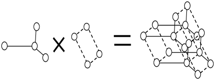
The Cartesian product $G_{1}\times\ldots\times G_{r}$ of elastic graphs $G_{1},\ldots G_{r}$ is an elastic graph with vertex set $V_{1}\times\ldots\times V_{r}$. Let $1\leq i\leq r$ and $v_{j}\in V_{j}$ ($j\neq i$). For this set of vertices, $\{v_{j}\}_{j\neq i}$, a copy of $G_{i}$ in $G_{1}\times\ldots\times G_{r}$ is defined with vertices $(v_{1},\ldots v_{i-1},v,v_{i+1},\ldots v_{r})$ ($v\in V_{i}$), edges ((v_1,…v_i-1, v, v_i+1, …v_r), (v_1,…v_i-1, v’, v_i+1, …v_r)),    (v,v’) ∈E_i   , and, similarly, $k$-stars of the form $(v_{1},\ldots v_{i-1},S_{k},v_{i+1},\ldots v_{r})$, where $S_{k}$ is a $k$-star in $G_{i}$. For any $G_{i}$ there are $\prod_{j,j\neq i}|V_{j}|$ copies of $G_{i}$ in $G$. Sets of edges and $k$-stars for Cartesian product are unions of that set through all copies of all factors. A map $\phi:V_{1}\times\ldots\times V_{r}\to R^{m}$ maps all the copies of factors into $R^{m}$ too. The energy of the elastic graph product is the energy sum of all factor copies. It is, of course, a quadratic functional of $\phi$.

The only difference between the construction of general elastic graphs and factorized graphs is in the application of the transformations. For factorized graphs, we apply them to factors. This approach significantly reduces the amount of trials in selection of the optimal application. The simple grammar with two rules, “add a node to a node, or bisect an edge,” is also powerful here, it produces products of primitive elastic trees. For such a product, the elastic structure is defined by the topology of the factors.

3 Principal Trees (Branching Principal Curves)

3.1 Simple Graph Grammar (“Add a Node”, “Bisect an Edge”)

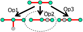
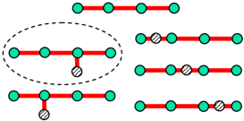
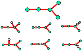
As a simple (but already rather powerful) example we use a system of two transformations: “add a node to a node” and “bisect an edge.” These transformations act on a class of primitive elastic graphs: all non-terminal nodes with $k$ edges are centers of elastic k-stars, which form all the $k$-stars of the graph. For a primitive elastic graph, the number of stars is equal to the number of non-terminal nodes – the graph topology prescribes the elastic structure.

a)                                             b)

c)

Figure 2: Illustration of the simple “add node to a node” or “bisect an edge” graph grammar application. a) We start with a simple 2-star from which one can generate three distinct graphs shown. The “Op1” operation is adding a node to a node, operations “Op1” and “Op2” are edge bisections (here they are topologically equivalent to adding a node to a terminal node of the initial 2-star). For illustration let us suppose that the “Op2” operation gives the biggest elastic energy decrement, thus it is the “optimal” operation. b) From the graph obtained one can generate 5 distinct graphs and choose the optimal one. c) The process is continued until a definite number of nodes is inserted

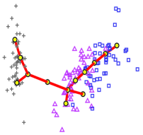
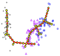
The transformation “add a node” can be applied to any vertex $y$ of $G$: add a new node $z$ and a new edge $(y,z)$. The transformation “bisect an edge” is applicable to any pair of graph vertices $y,y^{\prime}$ connected by an edge $(y,y^{\prime})$: Delete edge $(y,y^{\prime})$, add a vertex $z$ and two edges, $(y,z)$ and $(z,y^{\prime})$. The transformation of the elastic structure (change in the star list) is induced by the change of topology, because the elastic graph is primitive. This two–transformation grammar with energy minimization builds principal trees (and principal curves, as a particular case) for datasets. A couple of examples are presented on Fig. 3. For applications, it is useful to associate one-dimensional continua with these principal trees. Such a continuum consists of node images $\phi(y)$ and of pieces of straight lines that connect images of linked nodes.

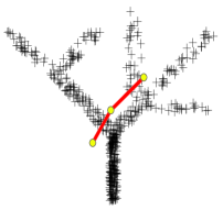
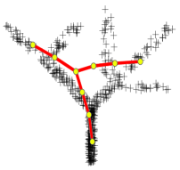
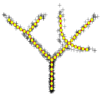
Iteration 1                     Iteration 5                     Iteration 50

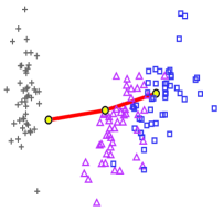
Iteration 1                     Iteration 10                     Iteration 50

Figure 3: Applying a simple “add a node to a node or bisect an edge” grammar to construct principal elastic trees (one node is added per iteration). Upper row: an example of two-dimensional branching distribution of points. Lower row: the classical benchmark, the “iris” four-dimensional dataset (point shapes distinguish three classes of points), the dataset and principal tree are presented in projection onto the plane of the first two principal components

3.2 Visualization of Data Using
“Metro Map” Two-Dimensional Tree Layout

A principal tree is embedded into a multidimensional data space. It approximates the data so that one can project points from the multidimensional space into the closest node of the tree (other projectors are also possible, for example, see the accompanying paper GorZin2007Springer ). The tree by its construction is a one-dimensional object, so this projection performs dimension reduction of the multidimensional data. The question is how to represent the result of this projection? For example, how to produce a tree layout on the two-dimensional surface of paper sheet? Of course, there are many ways to layout a tree on a plane. It is always possible to find a tree layout without edge intersection. But it would be very nice if both some tree properties and global distance relations would be represented using the layout. We can require that

1) In a two-dimensional layout, all k-stars should be represented equiangular, because the ideal configuration of a k-star with small energy is equiangular and with equal edge lengths.

2) The edge lengths should be proportional to their length in the multi-dimensional embedding; thus one can represent between-node distances.

Figure 4: Two-dimensional layout of the principal tree constructed for the iris dataset. In this layout all stars are equiangular and the edge lengths are proportional to the real edge lengths in the multidimensional space. The data points were projected into the closest tree nodes. The circle radii are proportional to the number of points projected into each node. Three different colors (or gray tints on the gray version of the image) denote three point classes. If points of different classes were projected into the same tree node then the number of points of every class is visualized by the pie diagram

This defines a tree layout up to global rotation and scaling and also up to changing the order of leaves in every $k$-star. We can change this order to eliminate edge intersections, but the result can not be guaranteed. In order to represent the global distance structure, we found that a good approximation for the order of $k$-star leaves can be taken from the projection of every $k$-star on the linear principal plane calculated for all data points, or on the local principal plane in the vicinity of the $k$-star, calculated only for the points close to this star.

In the current implementation of the method, after defining the initial approximation, a user manually modifies the layout switching the order of $k$-star leaves to get rid of edge intersections. The edge lengths are also modifiable. Usually it is possible to avoid edge intersections in the layout after a small number of initial layout modifications. This process could be also fully automated, by a greedy optimization algorithm, for example, but this possibility is not yet implemented.

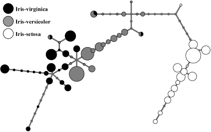
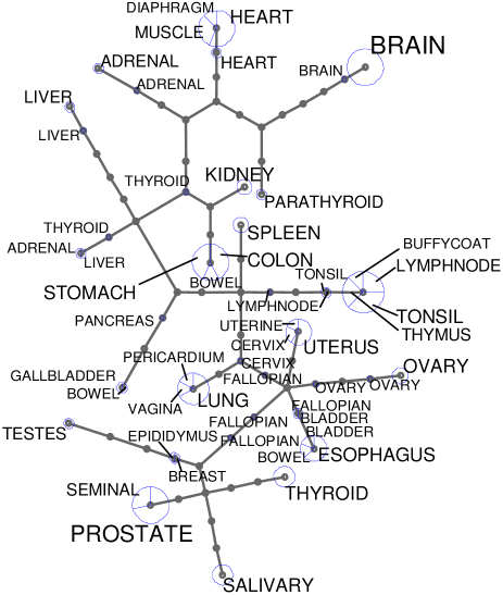
The point projections are then represented as pie diagrams, where the size of the diagram reflects the number of points projected into the corresponding tree node. The sectors of the diagram allow us to show proportions of points of different classes projected into the node (see an example on Fig. 4).

We call this type of visualization a “metro map” since it is a schematic and “idealized” representation of the tree and the data distribution with inevitable distortions made to produce a nice 2D layout, but using this map one can still estimate the distance from a point (tree node) to a point passing through other points. This map is inherently unrooted (as a real metro map). It is useful to compare this metaphor with trees produced by hierarchical clustering where the metaphor is closer to a “genealogy tree”.

3.3 Example of Principal Cubic Complex:
Product of Principal Trees

Principal trees are one-dimensional objects. To illustrate the idea of a $d$-dimensional principal cubic complex that is a cartesian product of graphs (see Fig. 1), we implemented an algorithm, constructing products of principal trees. The pseudocode for this algorithm is provided below:

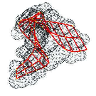
Thus, the structure of a principal cubic complex is defined by its dimension and the graph grammar applied for its construction. A simple example of 2-dimensional principal tree, i.e. cubic complex constructed with the simplest “add a node or bisect an edge” grammar (see Fig. 2) is given in Fig. 5. Here the cubic complex is constructed for a distribution of points on the molecular surface of a fragment of a DNA molecule (compare with the application of the method of elastic maps to the same dataset, given in the accompanying paper GorZin2007Springer ). The method of topological grammars 9Gorban07AML “discovers” the double-helical structure of the DNA molecule. Note that in this example the energy optimization gave no branching in both factors (trees) and as a result we obtained a product of two simple poly-lines. In other situations, the resulting cubic complex could be more complicated, with branching in one or both factors.

Figure 5: A cubic complex (2-dimensional, “add a node, bisect an edge” graph grammar) constructed for a distribution of points on the Van-der-Waals surface of a fragment of a DNA molecule (dots). The result is the product of two unbranched trees which “discovers” the double-helical DNA structure

4 Analysis of the Universal 7-Cluster Structure
of Bacterial Genomes

In this section we describe the application of the method of topological grammars to the analysis of the cluster structure of bacterial genomes. This structure appears as a result of projecting a genome sequence into a multidimensional space of short word frequencies 7cluPhA ; 7clulast . In particular, we show that a one-dimensional principal tree can reveal a signal invisible when three-dimensional PCA is applied.

4.1 Brief Introduction

One of the most exciting problems in modern science is to understand the organization of living matter by reading genomic sequences. The information that is needed for a living cell to function is encoded in a long molecule of DNA. It can be presented as a text that has only four letters A, C, G and T.

One distinctive message in a genomic sequence is a piece of text, called a gene. Genes can be oriented in the sequence in the forward and backward directions. In bacterial genomes genes are always continuous from their start to the stop signal.

It was one of many great discoveries of the twentieth century that biological information is encoded in genes by means of triplets of letters, called codons in the biological literature. In the famous paper by Crick et al. Crick61 , this fact was proven by genetic experiments carried out on bacteria mutants.

In nature, there is a special mechanism that is designed to read genes. It is evident that as the information is encoded by non-overlapping triplets, it is critical for this mechanism to start reading a gene without a shift, from the first letter of the first codon to the last one; otherwise, the information decoded will be completely corrupted.

A word is any continuous piece of text that contains several subsequent letters. As there are no spaces in the text, separation into words is not unique.

The method we use to “decipher” genomic sequences is the following. We clip the whole text into fragments of 300 letters in length and calculate the frequencies of short words (of length 1–4) inside every fragment. This gives a description of the text in the form of a numerical table (word frequency vs fragment number).

As there are only four letters, there are four possible words of length $1$ (singlets), $16=4^{2}$ possible words of length $2$ (duplets), $64=4^{3}$ possible words of length $3$ (triplets) and $256=4^{4}$ possible words of length $4$ (quadruplets). The first table contains four columns (frequency of every singlet) and the number of rows equals the number of fragments. The second table has 16 columns and the same number of rows, and so on.

These tables can be visualized by means of standard PCA. The result of such visualization is given on Fig. 6. As one can see from PCA plots, counting triplets gives an interesting flower-like pattern (described in details in 7cluPhA ; 7clulast ), which can be interpreted as the existence of non-overlapping triplet code.

The triplet picture evidently contains 7 clusters, and it is more structured in the space than 1,2- and 4-tuples. To understand the 7-cluster structure, let us make some explanations.

Let us blindly cut the text into fragments. Any fragment can contain: (a) piece of gene in the forward direction; (b) piece of gene in the backward direction; (c) no genes (non-coding part); (d) a mixture of coding and non-coding.

Consider case (a). The fragment can overlap with a gene in three possible ways, with three possible shifts. If we start to read the information one triplet after another starting from the first letter of the fragment then we can read the gene correctly only if the fragment overlaps it with a correct shift. In general, if the start of the fragment is chosen randomly then we can read the gene in three possible ways. Thus, case a) generates three possible frequency distributions, “shifted” one with respect to another.

Case (b) is quite analogous and also gives three possible triplet distributions. They are not quite independent from the ones obtained at the step (a) for the following reason. The frequency of triplets is in fact the same as in the case (a), the difference is the triplets are read “from the end to the beginning” which produces a kind of mirror reflection of the triplet distributions from the case (a).

Case (c) will produce only one distribution which will be symmetrical with respect to the “shifts” (or rotations) in the first two cases, and there is a hypothesis that this is a result of genomic sequence evolution. Let us explain it.

The vitality of a bacterium depends on the correct functioning of all biological mechanisms. All these mechanisms are encoded in genes, and if something wrong happens with gene sequences (for example there is an error when DNA is duplicated), then the organism risks becoming non-vital. Nothing is perfect in our world and errors happen all the time, and in the DNA duplication process as well. These errors are called mutations.

The most dangerous mutations are those which change the reading frame, i.e. letter deletions or insertions. If such a mutation happens in the middle of a gene sequence, the rest of the gene becomes corrupted: the reading mechanism (which reads the triplets one by one and does not know about the mutation) will read it with a shift. Because of this the organisms with such mutations often die without leaving their off-spring. Conversely, if such a mutation happens in the non-coding part, where there are no genes, this does not lead to problems, and the organism leaves off-spring. Thus such mutations are constantly accumulated in the non-coding part making all three phase-specific distributions identical. The (d) case also produces mix of triplet distributions.

As a result, we have three distributions for case (a), three for case (b) and one, symmetrical for the “non-coding” fragments (case (c)). Because of natural statistical deviations and other reasons we have 7 clusters of points in the multidimensional space of triplet frequencies.

a)	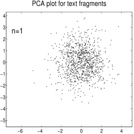b)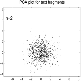
c)	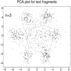d)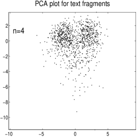

Figure 6: PCA plots of word frequencies of different length. In c) one can see the most structured distribution. The structure is interpreted as the existence of a non-overlapping triplet code

4.2 Visualization of the 7-Cluster Structure

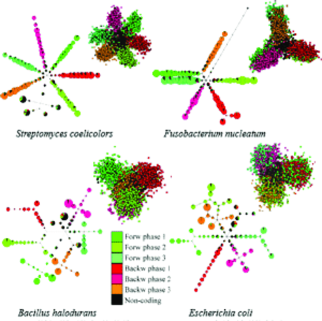
It happens that the flower-like pattern of the 7-cluster structure is only one of several possible 7cluPhA ; 7clulast when we observe many bacterial genomes. Four “typical” configurations of 7-clusters observed in bacterial genomes are shown on Fig. 7.

Among these four typical configurations, there is one called “degenerative” (Escherichia coli in Fig. 7). In this configuration three clusters corresponding to reading genes in the backward direction (reddish clusters) overlap with three clusters corresponding to reading genes in the forward direction (greenish clusters), when the distribution is projected in the three-dimensional space of the first principal components. It allows us to make a hypothesis that the usage of triplets is symmetrical with respect to the operation of “complementary reversal”.

However, for a real genome of Escherichia coli, we can observe, using the “metro map” representation, that the clusters are in fact rather well separated in space. This signal is completely hidden in the PCA plot. This is even more interesting since we are comparing data approximation and visualization by a one-dimensional object (principal tree) with one made by a three-dimensional linear manifold (PCA).

Figure 7: Seven cluster structures presented for 4 selected genomes. A genome is represented as a collection of points (text fragments represented by their triplet frequencies) in a multidimensional space. Color codes correspond to 6 possible frameshifts when a random fragment overlaps with a gene (3 in the forward and 3 in the backward direction of the gene), and the black color corresponds to non-coding regions. For every genome a principal tree (“metro map” layout) is shown together with 2D PCA projection of the data distribution. Note that the clusters that are mixed in the PCA plot for Escherichia coli (they remain mixed in 3D PCA as well, see web7clusters ) are well separated on the “metro map”

5 Visualization of Microarray Data

5.1 Dataset Used

DNA microarray data is a rich source of information for molecular biology (for a recent overview, read 9Leung2003 ). This technology found numerous applications in understanding various biological processes including cancer. It allows screening of the expression of all genes simultaneously in a cell exposed to some specific conditions (for example, stress, cancer, normal conditions). Obtaining a sufficient number of observations (chips), one can construct a table of ”samples vs genes”, containing logarithms of the expression levels of typically several thousands ($n$) of genes in typically several tens ($m$) of samples.

We use data published in 9Shyamsundar2005 containing gene expression values for 10401 genes in 103 samples of normal human tissues. The sample labels correspond to the tissue type from which the sample was taken. This dataset was proposed for analysis for the participants of the international workshop ”Principal manifolds-2006” which took place in Leicester, UK, in August of 2006. It can be downloaded from the workshop web-page 9PM2006Webpage .

5.2 Principal Tree of Human Tissues

On Fig. 8 a metro map representation of the principal tree calculated for the human tissue data is shown. To reduce the computation time we first calculated a new spatial basis by calculating 103 linear principal components and projected samples from the full-dimensional space into this basis. The missing values in the dataset were treated as described in the accompanying paper GorZin2007Springer (a data point with missing value(s) is represented as a line or a (hyper)plane parallel to the corresponding coordinate axes, for which we have missing information, and then projected into the closest point on the linear manifold). The principal tree was then constructed using the vdaoengine Java package available from the authors by request. We stopped construction of the optimal principal tree when 70 nodes were added to the tree.

One can see from the figure that most of the tissues are correctly clustered on the tree. Moreover, tissues of similar origin are grouped closely.

Figure 8: Principal tree of human tissues, constructed from the gene expression microarray data. The size of the circles corresponds to the number of points projected into this node. The sectors show the proportion of different tissue types projected into a node

6 Discussion

In the continuum representation, factors are one-dimensional continua, hence, a product of $r$ factors is represented as an $r$-dimensional cubic complex CubMatPol that is glued together from $r$-dimensional parallelepipeds (“cubes”). Thus, the factorized principal elastic graphs generate a new and, as we can estimate now, useful construction: a principal cubic complex. One of the obvious benefits from this construction is adaptive dimension: the grammar approach with energy optimization develops the necessary number of non-trivial factors, and not more. These complexes can approximate multidimensional datasets with complex, but still low-dimensional topology. The topology of the complex is not prescribed, but adaptive. In that sense, they are even more flexible than SOMs. The whole approach can be interpreted as an intermediate between absolutely flexible neural gas NeuralGaz and significantly more restrictive elastic map GorZinComp2005 . It includes as simple limit cases the $k$-means clustering algorithm (low elasticity moduli) and classical PCA (high $\mu$ for $S_{2}$ and $\mu\to\infty$ for $S_{k}$, $k>2$).

We demonstrated how application of the simplest “add a node, bisect an edge” grammar leads to the construction of a useful “principal tree” object (more precisely, branching principal curve) which can be advantageous over the application of customary linear PCA. Of course, more work is required to evaluate all advantages and disadvantages which this approach gives in comparison with existing and widely used techniques (for example, with hierarchical clustering). However, it is clear that the principal tree approach accompanied by the “metro map” representation of data, can provide additional insights into understanding the structure of complex data distributions and can be most suitable in some particular applications.

References

- (1) Bishop, C.M., Svensén, M., and Williams, C.K.I.: GTM: The generative topographic mapping. Neural Computation 10 (1), 215–234 (1998)
- (2) Crick, F.H.C., Barnett, L., Brenner, S., and Watts-Tobin, R.J.: General nature of the genetic code for proteins. Nature, 192, 1227–1232 (1961)
- (3) Dergachev, V.A., Gorban, A.N., Rossiev, A.A., Karimova, L.M., Kuandykov, E.B., Makarenko, N.G., and Steier, P.: The filling of gaps in geophysical time series by artificial neural networks Radiocarbon 43, 2A, 365–371 (2001)
- (4) Einbeck, J., Tutz, G., and Evers, L.: Local principal curves. Statistics and Computing, 15, 301–313 (2005)
- (5) Erwin, E., Obermayer, K., and Schulten, K.: Self-organizing maps: ordering, convergence properties and energy functions. Biological Cybernetics 67, 47–55 (1992)
- (6) Gorban, A.N., Popova, T.G., and Zinovyev, A.Yu.: Codon usage trajectories and 7-cluster structure of 143 complete bacterial genomic sequences. Physica A: Statistical and Theoretical Physics, 353, 365-387 (2005)
- (7) Gorban, A.N., Zinovyev, A.Yu., and Popova, T.G.: Four basic symmetry types in the universal 7-cluster structure of 143 complete bacterial genomic sequences. In Silico Biology 5 0025 (2005)
- (8) Gorban, A.N. and Rossiev, A.A.: Neural network iterative method of principal curves for data with gaps. Journal of Computer and System Sciences International 38 (5), 825–831 (1999)
- (9) Gorban, A.N, Sumner, N.R. and Zinovyev, A.Y.: Topological grammars for data approximation, Applied Mathematics Letters 20 (4), 382–386 (2005)
-
(10)
Gorban, A.N. and Zinovyev, A.Y.: Visualization of data by method
of elastic maps and its applications in genomics, economics and
sociology Preprint of Institut des Hautes Etudes Scientiques,
M/01/36 (2001)
http://www.ihes.fr/PREPRINTS/M01/Resu/resu-M01-36.html - (11) Gorban, A.N. and Zinovyev, A.Y.: Method of elastic maps and its applications in data visualization and data modeling. International Journal of Computing Anticipatory Systems, CHAOS, 12, 353–369 (2001)
- (12) Gorban, A.N., Zinovyev, A.Yu. and Wunsch, D.C.: Application of the method of elastic maps in analysis of genetic texts. In: Proceedings of International Joint Conference on Neural Networks (IJCNN). Portland, Oregon (2003).
- (13) Gorban, A.N., Zinovyev, A.Yu. and Pitenko, A.A.: Visualization of data using method of elastic maps (in Russian). Informatsionnie technologii 6, 26–35 (2000)
- (14) Gorban, A. and Zinovyev, A.: Elastic Principal Graphs and Manifolds and their Practical Applications. Computing 75, 359–379 (2005)
- (15) Gorban, A.N. and Zinovyev, A.Y.: Elastic maps and nets for approximating principal manifolds and their application to microarray data visualization. In this book.
- (16) Gusev, A.: Finite element mapping for spring network representations of the mechanics of solids. Phys. Rev. Lett. 93 (2), 034302 (2004)
- (17) Hastie, T. and Stuetzle, W.: Principal curves. Journal of the American Statistical Association 84 (406) (1989), 502–516 (1989)
- (18) Kégl, B. and Krzyzak, A.: Piecewise linear skeletonization using principal curves. IEEE Transactions on Pattern Analysis and Machine Intelligence 24 (1), 59–74 (2002)
- (19) Kohonen, T.: Self-organized formation of topologically correct feature maps. Biological Cybernetics 43, 59–69 (1982)
- (20) Leung, Y.F. and Cavalieri, D.: Fundamentals of cDNA microarray data analysis. Trends Genet. 19 (11), 649–659 (2003)
- (21) Löwe, M.: Algebraic approach to single–pushout graph transformation. Theor. Comp. Sci. 109, 181–224 (1993)
- (22) Martinetz, T.M., Berkovich, S.G., and Schulten K.J.: Neural-gas network for vector quantization and its application to time-series prediction. IEEE Transactions on Neural Networks, 4 4, 558–569 (1993)
- (23) Matveev, S. and Polyak, M.: Cubic complexes and finite type invariants. In: Geometry & Topology Monographs, Vol. 4: Invariants of knots and 3-manifolds. Kyoto, 215–233 (2001)
- (24) Mulier, F. and Cherkassky, V.: Self-organization as an iterative kernel smoothing process. Neural Computation 7, 1165–1177 (1995)
- (25) “Principal manifolds for data cartography and dimension reduction”, Leicester, UK, August 2006. A web-page with test microarrays datasets provided for participants of the workshop: http://www.ihes.fr/zinovyev/princmanif2006
- (26) Pearson, K.: On lines and planes of closest fit to systems of points in space. Philosophical Magazine, series 6 (2), 559–572 (1901)
- (27) Shyamsundar, R., Kim, Y.H., Higgins, J.P. et al.: A DNA microarray survey of gene expression in normal human tissues. Genome Biology, 6, R22 (2005)
- (28) Nagl, M.: Formal languages of labelled graphs: Computing, 16, 113–137 (1976)
- (29) Ritter, H., Martinetz, T. and Schulten, K.: Neural Computation and Self-Organizing Maps: An Introduction. Addison-Wesley Reading, Massachusetts (1992)
- (30) Zinovyev, A.: Visualization of Multidimensional Data. Krasnoyarsk State University Press Publ. (2000)
- (31) Zinovyev, A.Yu., Gorban, A.N. and Popova, T.G.: Self-organizing approach for automated gene identification. Open Systems and Information Dynamics 10 (4), 321–333 (2003)
- (32) Cluster structures in genomic word frequency distributions. Web-site with supplementary materials. http://www.ihes.fr/zinovyev/7clusters/index.htm