Elastic Maps and Nets
for Approximating Principal Manifolds
and Their Application
to Microarray Data Visualization

Abstract

Principal manifolds are defined as lines or surfaces passing through “the middle” of data distribution. Linear principal manifolds (Principal Components Analysis) are routinely used for dimension reduction, noise filtering and data visualization. Recently, methods for constructing non-linear principal manifolds were proposed, including our elastic maps approach which is based on a physical analogy with elastic membranes. We have developed a general geometric framework for constructing “principal objects” of various dimensions and topologies with the simplest quadratic form of the smoothness penalty which allows very effective parallel implementations. Our approach is implemented in three programming languages (C++, Java and Delphi) with two graphical user interfaces (VidaExpert and ViMiDa applications). In this paper we overview the method of elastic maps and present in detail one of its major applications: the visualization of microarray data in bioinformatics. We show that the method of elastic maps outperforms linear PCA in terms of data approximation, representation of between-point distance structure, preservation of local point neighborhood and representing point classes in low-dimensional spaces.

1 Introduction and Overview

1.1 Fréchet Mean and Principal Objects:
K-Means, PCA, what else?

A fruitful development of the statistical theory in the 20th century was an observation made by Fréchet in 1948 Frechet48 about the non-applicability of the mean value calculation in many important applications when the space of multi-dimensional measurements is not linear. The simple formula $M(x)=(1/N)\sum_{i=1}^{N}x_{i}$ where $x=\{x_{i}\}$ does not work if data points $x$ are defined on a Riemannian manifold (then $M(x)$ can simply not be located on it) or the distance metric defined in the data space is not quadratic.

This led to an important generalization of the mean value notion as a set which minimizes mean-square distance to the set of data samples:

$$M_{F}(x)=\arg\,\min_{y\in D}\sum_{i}(dist(y,x_{i}))^{2}\;,$$ (1)

where $D$ is the space of data samples and $dist(x,y)$ is a distance function between two points in $D$.

The existence and uniqueness of the Fréchet mean (1) is not generally guaranteed, but in many applications (one of the most important is statistical analysis in the shape space, see Kendall89 ) it proves to be constructive. In vector spaces $M_{F}=M$ only in the case of Euclidean (more generally, quadratic) metrics, whereas (1) allows to define a mean value with an alternative choice of metric.

Let us look at Fréchet definition from a different angle. We would like to utilize such spaces $D$ in (1) that does not necessarily coincide with the space of data samples. Let us consider a space of objects such that one can measure distance from an object $y$ to a sample $x_{i}$. Thus, using (1) one can find one (or a set of) “mean” or “principal” object in this space with respect to the dataset $X$.

Interestingly, simple examples of “principal objects” are equivalent to application of very well-known methods in statistical data analysis.

For example, let us consider $D$ as a space of $k$-tuples, i.e. $k$-element sets of vectors in $R^{m}$ (centroids), where $m$ is the dimension of the data space, and define distance between $y\in D$ and a point $x_{i}\in R^{m}$ as

$$dist(y,x_{i})=\min_{k=1..k}\|y_{k}-x_{i}\|\;,$$ (2)

where $y_{i}$ is the $i$th vector in the $k$-tuple $y$. Then the Fréchet mean corresponds to the optimal positions of centroids in the $K$-means clustering problem. Detailed discussion of the data approximation (“recovering”) approach with application to clustering is presented in 4Mi05 .

Another important example is the space $D$ of linear manifolds embedded in $R^{m}$. Let us consider a linear manifold $y$ defined in the parametric form $y(t)=a+bt$, where $t\in[-\infty;+\infty]$ is a parameter and $a,b\in R^{m}$. Let us define the function $dist(y,x)$ as the distance to the orthogonal projection of $x$ on $y$ (i.e., to the closest point on $y$):

$$dist(y,x_{i})=\min_{t\in[-\infty;+\infty]}\|y(t)-x_{i}\|\;.$$ (3)

Then, in the case of Euclidean metrics $\|y(t)-x\|^{2}=(y(t)-x)^{2}$ the “mean” manifold $y=M_{F}(x)$ corresponds exactly to the first principal component of $X$ (and this is exactly the first Pearson definition 4Pearson1901 ). Analogously, the $k$-dimensional “mean” linear manifold corresponds to the $k$-dimensional principal linear manifold.

The initial geometrical definition of the principal component as a line minimizing mean square distance from the data points has certain advantages in application. First, highly effective algorithms for its computation are proposed in the case of data spaces with very high dimension. Second, this definition is easily adapted to the case of incomplete data, as we show below.

In a certain sense, $K$-means clustering and linear principal manifolds are extreme cases of “principal objects”: the first one is maximally flexible with no particular structure, simply a $k$-tuple, while the second one presents a rigid linear manifold fitted to data. It is known that linear principal components (including the mean value itself, as a 0-dimensional principal object) are optimal data estimators only for gaussian data distributions. In practice we are often faced with non-gaussivities in the data and then linear PCA is optimal only in the class of linear estimators. It is possible to construct a “principal object” in-between these two extreme alternatives ($K$-Means vs PCA), such that it would be flexible enough to adapt to data non-gaussivity and still have some regular structure.

Elastic nets were developed in a series of papers Gorban01 ; GorbanRossiev99 ; GapsGRW ; GorbanVisPreprint01 ; GorbanCHAOS01 ; Gorban03 . By their construction, they are system of elastic springs embedded in the data space. This system forms a regular grid such that it can serve for approximation of some low-dimensional manifold. The elastic coefficients of this system allow the switch from completely unstructured $K$-means clustering (zero elasticity) to the estimators located closely to linear PCA manifolds (very rigid springs). With some intermediate values of the elasticity coefficients, this system effectively approximates non-linear principal manifolds which are briefly reviewed in the next section.

1.2 Principal Manifolds

Principal manifolds were introduced in PhD thesis of Hastie Hastie84 and then in the paper of Hastie and Stueltze HastieStuetzle89 as lines or surfaces passing through “the middle” of the data distribution. This intuitive definition was supported by a mathematical notion of self-consistency: every point of the principal manifold is a conditional mean of all points that are projected into this point. In the case of datasets only one or zero data points are projected in a typical point of the principal manifold, thus, one has to introduce smoothers that become an essential part of the principal manifold construction algorithms.

Since these pioneering works, many modifications and alternative definitions of principal manifolds have appeared in the literature. Theoretically, existence of self-consistent principal manifolds is not guaranteed for arbitrary probability distributions. Many alternative definitions were introduced (see, for example, KeglThesis99 ) in order to improve the situation and to allow the construction of principal curves (manifolds) for a distribution of points with several finite first moments. A computationally effective and robust algorithmic kernel for principal curve construction, called the Polygonal algorithm, was proposed by Kégl et al. Kegl99 . A variant of this strategy for constructing principal graphs was also formulated in the context of the skeletonization of hand-written digits Kegl02 . “Kernalised” version of PCA was developed in 4Scholkopf1998 . A general setting for constructing regularized principal manifolds was proposed in 4Smola1999 ; Smola2001 . In a practical example Smola2001 of oil flow data it was demonstrated that non-linear principal manifolds reveal point class structure better than the linear ones. Piece-wise construction of principal curves by fitting unconnected line segments was proposed in Verbeek00 .

Probably, most scientific and industrial applications of principal manifold methodology were implemented using the Kohonen Self-Organizing Maps (SOM) approach developed in the theory of neural networks Kohonen82 . These applications are too numerous to be mentioned here (see reviews in SOMbiblioPart1 ; SOMbiblioPart2 ; Yin2002 ; Yin2003 ): we only mention that SOMs and its numerous improvements, indeed, can provide principal manifold approximations (for example, see Mulier95 ; Ritter92 ) and are computationally effective. The disadvantage of this approach is that it is entirely based on heuristics; also it was shown that in the SOM strategy there does not exist any objective function that is minimized by the training process Erwin92 . These limitations were discussed in 4Bishop1998 , and the Generative Topographic Mapping (GTM) approach was proposed, in which a Gaussian mixture model defined on a regular grid and the explicit log likelihood cost function were utilized.

Since 1998 we have developed an approach for constructing principal manifolds based on a physical analogy with elastic membranes modeled by a system of springs. The idea of using the elastic energy functional for principal manifold construction in the context of neural network methodology was proposed in the mid 1990s (see Gorban98 ; GorbanRossiev99 and the bibliography there). Due to the simple quadratic form of the curvature penalty function, the algorithm proposed for minimization of elastic energy proved to be very computationally effective and allowed parallel implementations. Packages in three programming languages (C++, Java and Delphi) were developed Elmap ; VidaExpert ; VIMIDA together with graphical user interfaces (VidaExpert VidaExpert and ViMiDa VIMIDA ). The elastic map approach led to many practical applications, in particular in data visualization and missing data value recovery. It was applied for visualization of economic and sociological tables GorbanVisPreprint01 ; GorbanCHAOS01 ; GorbanInfo00 ; ZinovyevBook00 , to visualization of natural ZinovyevBook00 and genetic texts Gorban03 ; GorbanOpSys03 ; Zinovyev02 , recovering missing values in geophysical time series GapsDGRKM . Modifications of the algorithm and various adaptive optimization strategies were proposed for modeling molecular surfaces and contour extraction in images GorbanZinovyev05Computing . Recently the elastic maps approach was extended for construction of cubic complexes (objects more general than manifolds) in the framework of topological grammars Gorban07AML . The simplest type of grammar (“add a node”, “bisect an edge”) leads to construction of branching principal components (principal trees) that are described in the accompanying paper.

1.3 Elastic Functional and Elastic Nets

Let $G$ be a simple undirected graph with set of vertices $Y$ and set of edges $E$. For $k\geq 2$ a $k$-star in $G$ is a subgraph with $k+1$ vertices $y_{0,1,...,k}\in Y$ and $k$ edges $\{(y_{0},y_{i})|i=1,..,k\}\subset E$. Suppose that for each $k\geq 2$, a family $S_{k}$ of $k$-stars in $G$ has been selected. Then we define an elastic graph as a graph with selected families of $k$-starts $S_{k}$ and for which for all $E^{i}\in E$ and $S^{j}_{k}\in S_{k}$, the corresponding elasticity moduli $\lambda_{i}>0$ and $\mu_{kj}>0$ are defined.

Let $E^{(i)}(0)$, $E^{(i)}(1)$ denote two vertices of the graph edge $E^{(i)}$ and $S_{k}^{(j)}(0),...,S_{k}^{(j)}(k)$ denote vertices of a $k$-star $S_{k}^{(j)}$ (where $S_{k}^{(j)}(0)$ is the central vertex, to which all other vertices are connected). Let us consider a map $\phi:Y\rightarrow R^{m}$ which describes an embedding of the graph into a multidimensional space. The elastic energy of the graph embedding is defined as

$$U^{\phi}(G):=U^{\phi}_{E}(G)+U^{\phi}_{R}(G)\;,$$ (4)

$$U^{\phi}_{E}(G):=\sum_{E^{(}i)}\lambda_{i}\left\|\phi(E^{(i)}(0))-\phi(E^{(i)}(1))\right\|^{2}\;,$$ (5)

$$U^{\phi}_{R}(G):=\sum_{S^{(j)}_{k}}\mu_{kj}\left\|\sum_{i=1}^{k}\phi(S_{k}^{(j)}(i))-k\phi(S_{k}^{(j)}(0))\right\|^{2}\;.$$ (6)

This general definition of an elastic graph and its energy is used in Gorban07AML and in the accompanying paper to define elastic cubic complexes, a new interesting type of principal objects. In this paper we use elastic graphs to construct grid approximations to some regular manifolds. Because of this we limit ourselves to the case $k=2$ and consider graphs with nodes connected into some regular grids (see Fig. 1). In this case we will refer to $G$ as an elastic net.

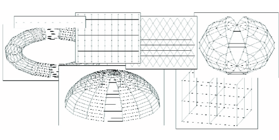
Figure 1: Elastic nets used in practice

The $2$-star is also called a rib (see Fig.2). The contribution $\mu_{j}\left\|\phi(S^{(j)}_{2}(1))+\phi(S^{(j)}_{2}(2))-2\phi(S^{(j)}_{2}(0))\right\|^{2}$ (in which one can recognize a discrete approximation of the second derivative squared) of the $j$th rib to the elastic energy equals zero only if the embedding of the central vertice is the average of its neighbours. Ribs introduce a simple quadratic penalty term on the non-linearity (in other words, complexity) of graph embedding.

Figure 2: A node, an edge and a rib (2-star)

How is the set ${S_{2}}$ chosen for an elastic net? In most of the cases this choice is natural and is dictated by the structure of the net. It is useful to consider another embedding of the graph $G$ in a low-dimensional space, where the graph has its “natural” form. For example, on Fig. 1 the regular rectangular grid is embedded into $R^{2}$ and $S_{2}$ is defined as all triples of adjacent collinear vertices.

We would like to find such a map $\phi$ that has low elastic energy and simultaneously approximates a set of data points $X$, where the approximation error is defined as the usual mean-square distance to the graph vertex positions in the data space. For a given map $\phi:Y\rightarrow R^{m}$ we divide the data set $X=\{x_{i}\}$ into subsets $\{K^{y_{j}}\}$, where $y_{j}\in Y$ is a vertex of the graph $G$. The set $K^{y_{j}}$ contains data points for which the node embedding $\phi(y_{j})$ is the closest one:

$$K^{y_{i}}=\{x_{i}|y_{j}=\arg\min_{y_{k}\in Y}\|y_{k}-x_{i}\|\}\;.$$ (7)

Then the approximation error (“approximation energy”) is defined as

$$U^{\phi}_{A}(G,X)=\frac{1}{\sum_{x\in X}w(x)}\sum_{y\in Y}\sum_{x\in K^{y}}w(x)\|x-\phi(y)\|^{2}\;,$$ (8)

where $w(x)\geq 0$ are the point weights. In the simplest case $w(x)=1$ but it might be useful to make some points ‘heavier’ or ‘lighter’ in the initial data.

The normalization factor ${1}/{\sum_{x\in X}w(x)}$ in (8) is needed for the law of large numbers: if $X$ is an i.i.d. sample for a distribution with probability density $\rho(x)$ and finite first two moments then there should exist a limit of $U^{\phi}_{A}(G,X)$ for $|X|\to\infty$. This can be easily proved for $w(x)\equiv 1$ or if $w(x)\geq 0$ is a bounded continuous function of point $x$. In the limit $|X|\to\infty$ the energy of approximation is

$$U^{\phi}_{A}(G,\rho)=\frac{1}{\mathbf{E}(w)}\int_{x\in V^{y}}w(x)\rho(x)\|x-\phi(y)\|^{2}\,\mathrm{d}^{m}x\;,$$ (9)

where $V^{y}=\{x\in R^{m}\,|y=\arg\min_{z\in Y}\|z-x\|\}$ is the Voronoi cell and $\mathbf{E}(m)=\int w(x)\rho(x)\,\mathrm{d}^{m}x$ is the expectation.

The optimal map $\phi_{opt}$ minimizes the total energy function (approximation+elastic energy):

$$U^{\phi}:=U^{\phi}_{A}(G,X)+U(G)^{\phi}\;.$$ (10)

To have a visual image of (10), one can imagine that every graph node $y_{j}$ is connected by elastic bonds to its closest data points in $K^{y_{j}}$ and simultaneously to the adjacent nodes (see Fig. 3).

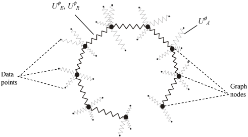
Figure 3: Energy of elastic net

The values $\lambda_{i}$ and $\mu_{j}$ are the coefficients of stretching elasticity of every edge $E^{{\rm(}i{\rm)}}$ and of bending elasticity of every rib $S^{j}_{2}$. In the simplest case we have

$$\lambda_{1}=\lambda_{2}=...=\lambda_{s}=\lambda(s),\quad\mu_{1}=\mu_{2}=...=\mu_{r}=\mu(r)\;,$$

where $s$ and $r$ are the numbers of edges and ribs correspondingly. To obtain $\lambda(s)$ and $\mu(r)$ dependencies we simplify the task and consider the case of a regular, evenly stretched and evenly bent grid. Let us consider a lattice of nodes of “internal” dimension $d$ ($d=1$ in the case of a polyline, $d=2$ in case of a rectangular grid, $d=3$ in the case of a cubical grid and so on). Let the “volume” of the lattice be equal to $V$. Then the edge length equals $(V/s)^{1/d}$. Having in mind that for typical regular grids $r\approx s$, we can calculate the smoothing parts of the functional: $U_{E}$$\sim$ $\lambda s^{{\frac{{d-2}}{{d}}}}$, $U_{R}$$\sim$ $\mu r^{{\frac{{d-2}}{{d}}}}$. Then in the case where we want $U_{R},U_{E}$ to be independent on the grid “resolution”,

$$\lambda=\lambda_{0}s^{{\frac{{2-d}}{{d}}}},\quad\mu=\mu_{0}r^{{\frac{{2-d}}{{d}}}}\;,$$ (11)

where $\lambda_{0}$, $\mu_{0}$ are elasticity parameters. This calculation is not applicable, of course, for the general case of any graph. The dimension in this case can not be easily defined and, in practical applications, the $\lambda_{i}$, $\mu_{i}$ are often made different in different parts of a graph according to some adaptation strategy (see below).

The elastic net approximates the cloud of data points and has regular properties. Minimization of the $U^{\phi}_{A}$ term provides approximation, the $U_{E}^{\phi}$ penalizes the total length (or, indirectly, “square”, “volume”, etc.) of the net and $U_{R}^{\phi}$ is a smoothing term, preventing the net from folding and twisting.

Other forms of $U_{R}^{\phi}$ are also used, in particular in the Polygonal algorithm Kegl99 . There exists a simple justification for the quadratic form of $U_{R}^{\phi}$ in (4): it is the simplest non-linearity penalty (which corresponds to a simple approximation of the second derivative). All other variants might be more effective in various specific applications but will be more and more close to our choice of $U_{R}^{\phi}$ with increasing grid resolution.

2 Optimization of Elastic Nets for Data Approximation

2.1 Basic Optimization Algorithm

Finding the globally optimal map $\phi$ is not an easy problem. In practice we can apply the splitting optimization strategy similar to $K$-means clustering. The optimization is done iteratively, with two steps at each iteration: 1) Determining $\{K^{y_{j}}\}$ for a given $\phi$ and 2) optimizing $\phi$ for a given $\{K^{y_{j}}\}$.

In order to perform the map optimization step 2 we derive the system of algebraic linear equations to be solved. Data points are separated in $K^{y_{j}},\;j=1\ldots p$.

Let us denote

$$\Delta(x,y)={\left\{{\begin{array}[]{l}{1,\;x=y}\\ {0,\;x\neq y\;,}\\ \end{array}}\right.}$$

$$\Delta E^{ij}\equiv\Delta(E^{(i)}(0),y^{(j)})-\Delta(E^{(i)}(1),y^{(j)})\;,$$

$$\Delta R^{ij}\equiv\Delta(S^{(i)}(2),y^{(j)})+\Delta(S^{(i)}(1),y^{(j)})-2\Delta(S^{(i)}(0),y^{(j)})\;.$$

That is, $\Delta E^{ij}=1$ if $y^{j}=E^{(i)}(0)$, $\Delta E^{ij}=-1$ if $y^{j}=E^{(i)}(0)$, and $\Delta E^{ij}=0$ for all other $y^{j}$; $\Delta R^{ij}=1$ if $y^{j}=R^{(i)}(1)$ or $y^{j}=R^{(i)}(2)$, $\Delta R^{ij}=-2$ if $y^{j}=R^{(i)}(0)$, and $\Delta R^{ij}=0$ for all other $y^{j}$. After a short calculation we obtain the system of $p$ linear equations to find new positions of nodes in multidimensional space {$\phi(y^{i}),i=$1…p}:

$${\sum\limits_{k=1}^{p}a_{jk}\phi(y^{(k)})={\frac{{1}}{\sum_{x\in D}w(x)}}}{\sum\limits_{x\in K^{y_{j}}}{w(x)x}}\;,$$

where

$$a_{jk}=\frac{{n_{j}\delta_{jk}}}{\sum_{x\in D}w(x)}+e_{jk}+r_{jk}\;,\quad j=1\ldots p\;,$$ (12)

$\delta_{jk}$ is Kronecker’s $\delta$, and $n_{j}=\sum_{x\in K^{y_{j}}}{w(x)}$, $e_{jk}={\sum\limits_{i=1}^{s}{\lambda_{i}\Delta E^{ij}\Delta E^{ik}}}$, $r_{jk}={\sum\limits_{i=1}^{r}{\mu_{i}\Delta R^{ij}\Delta R^{ik}}}$. The values of $e_{jk}$ and $r_{jk}$ depend only on the structure of the grid. If the structure does not change then they are constant. Thus only the diagonal elements of the matrix (12) depend on the data set. The $a$ matrix has sparse structure for a typical grid used in practice. In practice it is advantageous to calculate directly only non-zero elements of the matrix and this simple procedure was described in GorbanZinovyev05Computing .

The process of minimization is interrupted if the change in $U^{\phi}$ becomes less than a small value $\varepsilon$ or after a fixed number of iterations.

As usual, we can only guarantee that the algorithm leads to a local minimum of the functional. Obtaining a solution close to the global minimum can be a non-trivial task, especially in the case where the initial position of the grid is very different from the expected (or unknown) optimal solution. In many practical situations the “softening” strategy can be used to obtain solutions with low energy levels. This strategy starts with “rigid” grids (small length, small bending and large $\lambda$, $\mu$ coefficients) at the beginning of the learning process and finishes with soft grids (small $\lambda$, $\mu$ values), Fig. 4. Thus, the training goes in several epochs, each epoch with its own grid rigidness. The process of “softening” is one of numerous heuristics that pretend to find the global minimum of the energy $U$ or rather a close configuration.

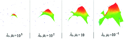
Figure 4: Training elastic net in several epochs (softening)

Nevertheless, for some artificial distributions (like the spiral point distribution, used as a test in many papers on principal curve construction) “softening” starting from any linear configuration of nodes does not lead to the expected solution. In this case, adaptive strategies, like “growing curve” (an analogue of what was used by Kégl in his polygonal algorithm Kegl99 or “growing surface” can be used to obtain suitable configuration of nodes.

We should mention the problem of good initial approximation for $\phi$, used to initialize the algorithm. For principal manifolds, one can start with the plane or the volume of several first principal components calculated for $X$ (as in 4Bishop1998 ; Gorban01 ), but other initializations could be also developed.

Another important remark is the choice of elastic coefficients $\mu$ and $\lambda$ such that they would give good approximation to a hypothetical “ideal” principal manifold. The standard strategies of using a training data subset or cross-validation could be used. For example, we can remove a certain percentage of points from the process of optimization and calculate approximation error on this test set for every “epoch” of manifold softening, thus stopping with the best parameter values. One should notice that despite the fact that we have two parameters, the “bending” elasticity parameter $\mu$ is more important for optimizing this “generalization” error, since it determines the curvature of $\phi$. The stretching elasticity parameter $\lambda$ is more important at the initial stage of net optimization since it (together with $\mu$) forces regularity of the node positions, making distances between neighboring nodes almost uniform along the net. For the final stage of the optimization process $\lambda$ can be even put to zero or some small value.

2.2 Missing Data Values

Our geometrical approach to the construction of principal manifolds allows us to deal very naturally with the missing values in the data. In bioinformatics this issue can be very important: in one of the examples below, there are missing values in almost any column and any row of the initial data table. When filling gaps with mean values is not a good solution to the problem, it is better to use principal objects for this purpose (the mean value itself is the 0-dimensional principal object).

The general idea is to be able to project a data point $x_{i}$ with missing values in some of its coordinates onto the principal object of the whole distribution $X$. In this case we can not represent $x_{i}$ as a simple vector anymore. If $x_{i}$ has $p$ missing values then it is natural to represent it as a linear manifold parallel to the $p$ coordinate axes for which the data values are missing: $x_{i}=[x_{i}^{0},...,t_{1},...,x_{i}^{k},...,t_{p},..,x_{i}^{m}],-\infty\leq t_{1},t_{2},...,t_{p}\geq\infty$. Then, for a principal manifold $y$, we can calculate the closest distance (or the intersection point) between two manifolds (the non-linear principal one and the linear one representing $x_{i}$) and use the coordinate values of the projected point. Theoretically, the reconstructed values are not unique, when $x_{i}$ and $y$ intersect in many points or even along lines, which gives several alternative solutions or even continuum for the reconstructed missing values. With increasing data dimension the probability of such intersections decreases.

2.3 Adaptive Strategies

The formulation of the method given above allows us to construct different adaptive strategies by playing with a) individual $\lambda_{i}$ and $\mu_{j}$ weights; b) the grid connection topology; c) the number of nodes.

This is a way of extending the approach significantly making it suitable for many practical applications.

First of all, let us define a basic operation on the grid, which allows inserting new nodes. Let us denote by N, S, R the sets of all nodes, edges and ribs respectively. Let us denote by C$(i)$ the set of all nodes which are connected to the $i$th node by an edge. If one has to insert a new node in the middle of an edge $I$, connecting two nodes $k$ and $l$, then the following operations have to be accomplished:

The grow-type strategy is applicable mainly to grids with planar topology (linear, rectangular, cubic grids). It consists of an iterative determination of those grid parts, which have the largest “load” and doubling the number of nodes in this part of the grid. The load can be defined in different ways. One natural way is to calculate the number of points that are projected onto the nodes. For linear grids the grow-type strategy consists of the following steps:

We should mention here also growing lump and growing flag strategies used in physical and chemical applications Grids ; CMIM . In the growing lump strategy we add new nodes uniformly at the boundary of the grid using a linear extrapolation of the grid embedding. Then the optimization step follows, and, after that, again the step of growing could be done.

For the principal flag one uses sufficiently regular grids, in which many points are situated on the coordinate lines, planes, etc. First, we build a one-dimensional grid (as a one-dimensional growing lump, for example). Then we add a new coordinate and start growing in new direction by adding lines. After that, we can add the third coordinate, and so on.

The break-type adaptive strategy changes individual rib weights in order to adapt the grid to those regions of data space where the “curvature” of data distribution has a break or is very different from the average value. It is particularly useful in applications of principal curves for contour extraction (see GorbanZinovyev05Computing ). For this purpose the following steps are performed:

To construct a “skeleton” for a two-dimensional point distribution, we apply a variant of local linear principal component analysis first, then connect local components into several connected parts and optimize the node positions afterwards. This procedure is robust and efficient in applications to clustering along curvilinear features and it was implemented as a part of the elmap package Elmap . The following steps are performed:

The adaptive strategies: “grow”, “break” and “principal” graphs can be combined and applied one after another. For example, the principal graph strategy can be followed by break-type weight adaptation or by grow-type grid adaptation.

3 Elastic Maps

3.1 Piecewise Linear Manifolds and Data Projectors

In the process of net optimization we use projection of data into the closest node. This allows us to improve the speed of the data projection step without loosing too much detail when the grid resolution is good enough. The effect of an estimation bias, connected with this type of projection, was observed in KeglThesis99 . In our approach the bias is indirectly reduced by utilizing the $U_{E}^{\phi}$ term that makes the grid almost isometric (having the same form, the grid will have lesser energy with equal edge lengths). For presentation of data points or for data compression, other projectors can be applied.

In applications we utilize a piece-wise linear projection onto the manifold. A natural way to do this is to introduce a set of simplexes on the grid (line segments for one-dimensional grids, triangles for two-dimensional grids, and tetrahedra for the 3D grids). Then one performs orthogonal projection onto this set. In order to avoid calculation of all distances to all simplexes, one can apply a simplified version of the projector: find the closest node of the grid and then consider only those simplexes that contain this node. This type of projection is used in the examples (Fig. 7-9).

Since the elastic net has a penalty on its length (and, for higher dimensions, indirectly, area, volume), the result of the optimization procedure is a bounded manifold, embedded in the cloud of data points. Because of this, if the penalty coefficient is big, many points can have projection on the boundary of the manifold. This can be undesirable, for example, in data visualization applications. To avoid this effect, a linear extrapolation of the bounded rectangular manifold (extending it by continuity in all directions) is used as a post-processing step.

Using piece-wise linear interpolation between nodes and linear extrapolation of the manifold is the simplest (hence computationally effective) possibility. It is equivalent to construction of piece-wise linear manifold. Other interpolation and extrapolation methods are also applicable, for example the use of Carleman’s formula Aizenberg93 ; Grids ; CMIM ; Gorban02 ; GapsGRW ; GapsDGRKM or using Lagrange polynomials Ritter93 , although they are more computationally expensive.

3.2 Iterative Data Approximation

An important limitation of many approaches that use grid approximations is that in practice it is feasible to construct only low-dimensional grids (no more than three-dimensional).

This limitation can be overcome in the additive iterative manner. After low-dimensional manifold $\phi$ is constructed, for every point $x$, its projection $P^{\phi}(x)$ onto the manifold is subtracted and new low-dimensional manifold is computed for the set of residues $\{x_{i}-P^{\phi}(x_{i})\}$. Thus a dataset can be approximated by a number of low-dimensional objects, each of them approximating the residues obtained from the approximation by the previous one. The norm of the residues at each iteration becomes smaller but is not guaranteed to become zero after a finite number of iterations, as in the case of linear manifolds.

4 Principal Manifold as Elastic Membrane

Let us discuss in more detail the central idea of our approach: using the metaphor of elastic membranes in the principal manifold construction algorithm. The system represented in Fig. 3 can be modeled as an elastic membrane with external forces applied to the nodes. In this section we consider the question of equivalence between our spring network system and realistic physical systems (evidently, we make comparison in 3D).

Spring meshes are widely used to create physical models of elastic media (for example, Born54 ). The advantages in comparison with the continuous approaches like the Finite Elements Method (FEM), are evident: computational speed, flexibility, the possibility to solve the inverse elasticity problem easily VanGelder97 .

Modeling elastic media by spring networks has a number of applications in computer graphics, where, for example, there is a need to create realistic models of soft tissues (human skin, as an example). In VanGelder97 it was shown that it is not generally possible to model elastic behavior of a membrane using spring meshes with simple scalar springs. In Xie02 the authors introduced complex system of penalizing terms to take into account angles between scalar springs as well as shear elasticity terms. This improved the results of modeling and has found applications in subdivision surface design.

In a recent paper Gusev04 a simple but important fact was noticed: every system of elastic finite elements could be represented by a system of springs, if we allow some springs to have negative elasticity coefficients. The energy of a $k$-star $S_{k}$ in $R^{m}$ with $y_{0}$ in the center and $k$ endpoints $y_{1,...,k}$ is $u_{S_{k}}=\mu_{S_{k}}(\sum_{i=1}^{k}y_{i}-ky_{0})^{2}$, or, in the spring representation, $u_{S_{k}}=k\mu_{S_{k}}\sum_{i=1}^{k}(y_{i}-y_{0})^{2}-\mu_{S_{k}}\sum_{i>j}(y_{i}-y_{j})^{2}$. Here we have $k$ positive springs with coefficients $k\mu_{S_{k}}$ and $k(k-1)/2$ negative springs with coefficients $-\mu_{S_{k}}$.

Let us slightly reformulate our problem to make it closer to the standard notations in the elasticity theory. We introduce the $m\times p$-dimensional vector of displacements, stacking all coordinates for every node:

$$u=\{u_{1}^{(1)};u_{2}^{(1)};..;u_{m}^{(1)};...;u_{1}^{(p)};u_{2}^{(p)};..;u_{m}^{(p)}\}^{T}\;,$$

where $m$ is dimension, $p$ is the number of nodes, $u_{i}^{(k)}$ is the $i$th component of the $k$th node displacement. The absolute positions of nodes are $y^{(k)}=\tilde{y}^{(k)}+u^{(k)}$, where $\tilde{y}^{(k)}$ are equilibrium (relaxed) positions. Then our minimization problem can be stated in the following generalized form:

$$\quad u^{T}Eu+D(u;x)\to\min\;,$$ (13)

where $E$ is a symmetric $(m\times p)\times(m\times p)$ element stiffness matrix. This matrix reflects the elastic properties of the spring network and has the following properties: 1) it is sparse; 2) it is invariant with respect to translations of the whole system (as a result, for any band of $m$ consecutive rows corresponding to a given node $k$, the sum of the m$m\times m$ off-diagonal blocks should always be equal to the corresponding diagonal block taken with the opposite sign). The $D(u;x)$ term describes how well the set of data $x$ is approximated by the spring network with the node displacement vector $u$. It can be interpreted as the energy of external forces applied to the nodes of the system. To minimize (13) we solve the problem of finding equilibrium between the elastic internal forces of the system (defined by $E$) and the external forces:

$$Eu=f,\;\;\;f=-{\frac{{1}}{{2}}}{\frac{{\partial}}{{\partial u}}}D(u;x)\;.$$ (14)

The matrix $E$ is assembled in a similar manner to that described in Subsec. 2.1. There is one important point: the springs have zero rest lengths, it means that equilibrium node positions are all in zero: $\tilde{y}^{(k)}=0,\;k=1..p$. The system behavior then can be described as “super-elastic”. From the point of view of data analysis it means that we do not impose any pre-defined shape on the data cloud structure.

For $D(u$;$x)$ we use the usual mean square distance measure, see (8): $D(u;x)=U^{\phi}_{A}$. The force applied to the $j$th node equals

$$f_{j}={\frac{{n^{(j)}}}{{N}}}\left({\tilde{x}^{(j)}-u^{(j)}}\right)\;,$$ (15)

where

$$\tilde{x}^{(j)}={\frac{{{\sum\limits_{x^{(i)}\in K^{y_{j}}}{w_{i}x^{(i)}}}}}{{n^{(j)}}}}\;,\;\;n^{(j)}={\sum\limits_{x^{(i)}\in K^{y_{j}}}{w_{i}}}\;,\;\;\;\;N={\sum\limits_{x^{(i)}}{w_{i}}}\;.$$

It is proportional to the vector connecting the $j$th node and the weighted average $\tilde{x}^{(j)}$ of the data points in $K^{{\rm(}j{\rm)}}$ (i.e., the average of the points that surround the $j$th node: see (7) for definition of $K^{y_{j}})$. The proportionality factor is simply the relative size of $K^{y_{j}}$. The linear structure of (15) allows us to move $u$ in the left part of the equation (15). Thus the problem is linear.

Now let us show how we can benefit from the definition (14) of the problem. First, we can introduce a pre-defined equilibrium shape of the manifold: this initial shape will be elastically deformed to fit the data. This approach corresponds to introducing a model into the data. Secondly, one can try to change the form (15) of the external forces applied to the system. In this way one can utilize other, more sophisticated approximation measures: for example, taking outliers into account.

Third, in three-dimensional applications one can benefit from existing solvers for finding equilibrium forms of elastic membranes. For multidimensional data point distributions one has to adapt them, but this adaptation is mostly formal.

Finally, there is a possibility of a hybrid approach: first, we utilize a “super-elastic” energy functional to find the initial approximation. Then we “fix” the result and define it as the equilibrium. Finally, we utilize a physical elastic functional to find elastic deformation of the equilibrium form to fit the data.

5 Method Implementation

For different applications we made several implementations of the elmap algorithm in the C++, Java and Delphi programming languages. All of them are available on-line Elmap ; VidaExpert ; VIMIDA or from the authors by request.

Two graphical user interfaces for constructing elastic maps have also been implemented. The first one is the VidaExpert stand-alone application VidaExpert which provides the possibility not only to construct elastic maps of various topologies but also to utilize linear and non-linear principal manifolds to visualize the results of other classical methods for data analysis (clustering, classification, etc.) VidaExpert has integrated 3D-viewer which allows data manipulations in interactive manner.

A Java implementation was also created VIMIDA , it was used to create a Java-applet ViMiDa (VIsualization of MIcroarray DAta). In the Bioinformatics Laboratory of Institut Curie (Paris) it is integrated with other high-throughput data analysis pipelines and serves as a data visualization user front-end (“one-click” solution). ViMiDa allows remote datasets to be downloaded and their visualization using linear or non-linear (elastic maps) principal manifolds.

6 Examples

6.1 Test Examples

In Fig. 5 we present two examples of 2D-datasets provided by Kégl.

The first dataset called spiral is one of the standard ways in the principal curve literature to show that one’s approach has better performance than the initial algorithm provided by Hastie and Stuetzle. As we have already mentioned, this is a bad case for optimization strategies, which start from a linear distribution of nodes and try to optimize all the nodes together in one loop. But the adaptive “growing curve” strategy, though being by order of magnitude slower than “softening”, finds the solution quite stably, with the exception of the region in the neighborhood of zero, where the spiral has very different (compared to the average) curvature.

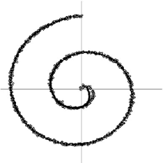
a) spiral b) large

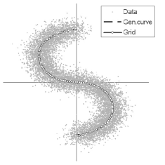
Figure 5: Two-dimensional examples of principal curves construction

The second dataset, called large presents a simple situation, despite the fact that it has comparatively large sample size (10000 points). The nature of this simplicity lies in the fact that the initial first principal component based approximation is already effective; the distribution is in fact quasilinear, since the principal curve can be unambiguously orthogonally projected onto a line. In Fig. 5b it is shown that the generating curve, which was used to produce this dataset, has been discovered almost perfectly and in a very short time.

Some other examples, in particular of application of the elastic graph       strategy are provided in GorbanZinovyev05Computing .

6.2 Modeling Molecular Surfaces

A molecular surface defines an effective region of space which is occupied by a molecule. For example, the Van-der-Waals molecular surface is formed by surrounding every atom in the molecule by a sphere of radius equal to the characteristic radius of the Van-der-Waals force. After all the interior points are eliminated, this forms a complicated non-smooth surface in 3D. In practice, this surface is sampled by a finite number of points.

Using principal manifolds methodology, we constructed a smooth approximation of such molecular surface for a small piece of a DNA molecule (several nucleotides long). For this we used slightly modified Rasmol source code Sayle92 (available from the authors by request).

First, we have made an approximation of this dataset by a 1D principal curve. Interestingly, this curve followed the backbone of the molecule, forming a spiral (see Fig. 6).

Second, we approximated the molecular surface by a 2D manifold. The topology of the surface is expected to be spherical, so we applied spherical topology of the elastic net for fitting. We should notice that since it is impossible to make the lengths of all edges equal for the sphere-like grid, corrections were performed for edge and rib weights during the grid initialization (shorter edges are given with larger weights proportionally and the same for the ribs).

As a result one gets a smooth principal manifold with spherical topology, approximating a rather complicated set of points. The result of applying principal manifold construction using the elmap Elmap package is shown in Fig. 6. The manifold allows us to introduce a global spherical coordinate system on the molecular surface. The advantage of this method is its ability to deal not only with star-like shapes as the spherical harmonic functions approach does (see, for example, Cai02 ) but also to model complex forms with cavities as well as non-spherical forms.

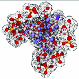
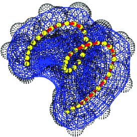
Figure 6: Approximating molecular surface of a simple fragment of DNA by 1D- and 2D- principal manifolds. On the left the molecule with molecular surface is shown, on the right the result of the approximation is shown. The small points are the points on the molecular surface, the big spiral is the 1D principal curve and the mesh is the 2D principal spherical manifold

6.3 Visualization of Microarray Data

DNA microarray data is a rich source of information for molecular biology (for a recent overview, see Leung2003 ). This technology found numerous applications in understanding various biological processes including cancer. It allows to screen simultaneously the expression of all genes in a cell exposed to some specific conditions (for example, stress, cancer, normal conditions). Obtaining a sufficient number of observations (chips), one can construct a table of “samples vs genes”, containing logarithms of the expression levels of, typically several thousands ($n$) of genes, in typically several tens ($m$) of samples.

The table can be represented as a set of points in two different spaces. Let us call them the “gene space” and the “sample space”. In the gene space every point (vector of dimension $m$) is a gene, characterized by its expression in $m$ samples. In the sample space every point is a sample (vector of dimension $n$), characterized by the expression profile of $n$ genes.

One of the basic features of microarray datasets is the fact that $n\gg~{}m$. This creates certain problems when one constructs a classifier in the “sample space”: for example, for standard Linear Discriminant Analysis, too many equivalent solutions for the problem are possible. Thus, some regularization of the classification problem is required (see, for example, Hastie05 ) and PCA-like techniques could be also used for such a purpose.

Here we provide results on the visualization of three microarray datasets in the “sample space” using elastic maps. We demonstrate that the two-dimensional principal manifolds outperform the corresponding two-dimensional principal planes, in terms of representation of big and small distances in the initial multidimensional space and visualizing class information.

Datasets used

For the participants of the international workshop “Principal manifolds-2006” which took place in Leicester, UK, in August of 2006, it was proposed to analyze three datasets containing published results of microarray technology application. These datasets can be downloaded from the workshop web-page PM2006Webpage .

Dataset I. Breast cancer microarrays. This dataset was published in Wang2005 and it contains 286 samples and expression values of 17816 genes. We processed the clinical information provided with this dataset and constructed three ab initio sample classifications:

GROUP: non-agressive (A) vs agressive (B) cancer;

ER: estrogen-receptor positive (ER+) vs estrogen-receptor negative (ER-) tumors;

TYPE: sub-typing of breast cancer (lumA, lumB, normal, errb2, basal and unclassified), based on the so-called Sorlie breast cancer molecular portraits (see Sorlie2000 ).

Dataset II. Bladder cancer microarrays. This dataset published in Dyrskjot03 contains 40 samples of bladder tumors. There are two ab initio sample classficitions:

TYPE: clinical classification of tumors (T1, T2+ anf Ta);

GRADE: tumor grade (2,3,4).

Dataset III. Collection of microarrays for normal human tissues. This dataset published in Shyamsundar2005 contains gene expression values in 103 samples of normal human tissues. The only ab initio sample classification corresponds to the tissue type from which the sample was taken.

Microarray datasets are inevitably incomplete: for example, there is a number of gaps (not reliably measured values) in Dataset III. Datasets I and II do not contain missing values (in Dataset I the missing values are recovered with use of some standard normalization method and in the Dataset II all gaps are filtered out). Dataset III is filtered in such a way that any row (gene) has at least 75% complete values of expression and every column has at least 80% of complete values. It is interesting to mention that missing values in Dataset III are distributed in such a way that almost every column and row contains a missing value. This means that missing value recovery is absolutely necessary for its analysis.

The original expression tables were processed to select 3000 genes with the most variable expression between samples. Thus the sample space has approximately equal dimensions (3000) for all three datasets. For every gene, the expression values were converted to $z$-values, i.e. every value was centered and divided by its standard deviation.

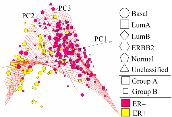
a)                                                     

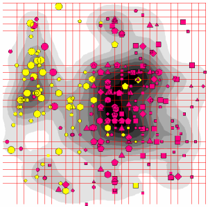
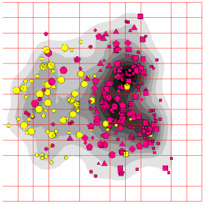
b) ELMap2D                                c) PCA2D

Figure 7: Visualization of Dataset I (breast cancer dataset) using elastic maps. Ab initio classifications are shown using points size (ER), shape (GROUP) and color (TYPE): a) configuration of nodes in the three-dimensional principal linear manifold. One clear feature is that the dataset is curved such that it can not be mapped adequately on a two-dimensional principal plane; b) the distribution of points in the internal non-linear manifold coordinates (ELMap2D) is shown together with an estimation of the two-dimensional density of points; c) the same as b), but for the linear two-dimensional manifold (PCA2D). One can notice that the “basal” breast cancer subtype is visualized more adequately with ELMap2D and some features of the distribution become better resolved in comparison to PCA2D

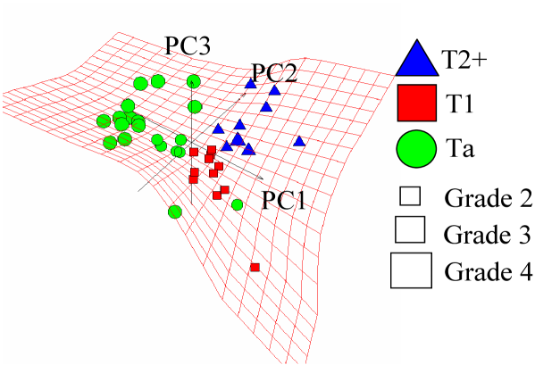
a)                                                     

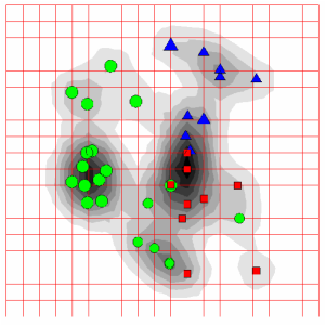
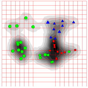
b) ELMap2D                                c) PCA2D

Figure 8: Visualization of Dataset II (bladder cancer dataset) using elastic maps. Ab initio classifications are shown using points size (GRADE) and color and shape (TYPE): a) configuration of nodes in the three-dimensional principal linear manifold; b) distribution of points in the internal manifold coordinates is shown together with an estimation of the two-dimensional density of points; c) the same as b), but for the linear manifold of the first two principal components (PCA2D). From all three datasets, Dataset II is “the least dimensional”, and the configurations of points are quite similar, although ELMap2D reveals some finer point grouping

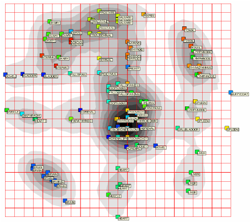
a) ELMap2D

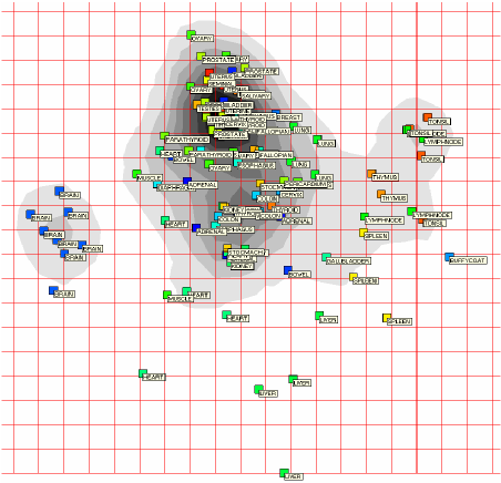
b) PCA2D

Figure 9: Visualization of Dataset III (normal tissue samples) using elastic maps (a) and two-dimensional PCA (b). Tissue names are shown using point labels. The ELMap2D image clearly gives a better “resolved” structure of classes, which is confirmed by quantitative measures of “class compactness” (see the text)

Principal manifolds for three datasets were approximated by the elastic map algorithm implemented in Java, the package VDAOEngine VIMIDA with a 2D rectangular node grid using the softening optimization strategy. The elastic nets were trained in two epochs: first one with $\lambda_{0}=0.1$ and $\mu_{0}=250$ and the second epoch with $\lambda_{0}=0.01$ and $\mu_{0}=30$. No optimization for the final value of $\mu_{0}$ was done. The resolution of grids was selected 15x15 for Dataset I and Dataset III and 10x10 for Dataset II. For post-processing we used linear extrapolation of the manifold, adding 5 node layers at each border of the manifold. An average time for elastic net computation using an ordinary PC was 1-5 minutes depending on the number of nodes in the net.

For data visualization and analysis we projected data points into their closest points on the manifold obtained by piece-wise linear interpolation between the nodes. The results are presented on Fig. 7-9. We show also the configuration of nodes projected into the three-dimensional principal linear manifold. This is done only for visualization of the fact that the elastic map is non-linear and usually better approximates the distribution of points in comparison with the linear principal plane. But one should not forget that the non-linear manifold is embedded in all dimensions of the high-dimensional space, not being limited to the space of the first principal components.

Mean-square distance error

By their construction, principal manifolds provide better approximation of data than the less flexible linear PCA. In the Table 1 we provide results of comparing the mean square distance error (MSE) of the datasets’ approximation by a two-dimensional non-linear elastic map and linear manifolds of various dimensions (1-5-dimensional and 10-dimensional) constructed with using standard PCA. In the case of elastic maps we calculate the distance of the projection to the closest point of the manifold as it is described in the section 3.1. The conclusion is that the two-dimensional principal manifolds outperform even four-dimensional linear PCA manifolds in their accuracy of data approximation.

Table 1: Mean square distance error (MSE) of data approximation by two-dimensional elastic maps (ELMap2D) and linear PCA manifolds of various dimensions (PC1-PC5,PC10). For linear principal components, the cumulative explained variation is also shown

Dataset	ELMap2D	PC1	PC2	PC3	PC4	PC5	PC10
Breast cancer MSE	48.1	52.6	50.7	49.3	48.4	47.6	45.3
Variation explained	-	7.9%	14.3%	19.0%	22.0%	24.6%	31.5%
Bladder cancer MSE	40.6	48.7	45.4	42.8	40.7	39.2	33.0
Variation explained	-	21.0%	31.4%	38.9%	44.8%	48.8%	63.8%
Normal tissues MSE	36.9	48.8	45.5	42.3	40.1	38.5	32.4
Variation explained	-	10.7%	19.1%	26.0%	30.3%	32.2%	40.7%

Natural PCA and distance mapping

Our second analysis answers the question of how successfully the structure of distances in the initial highly multidimensional space is reconstructed after projection into the low-dimensional space of the internal co-ordinates of the principal manifold. A possible indicator is the correlation coefficient between all pair-wise distances:

$$r=corr(d_{ij},\hat{d}_{ij})\;,$$ (16)

where $d_{ij}$ and $\hat{d}_{ij}$ are the pair-wise distances in the original high-dimensional space and the distances in the “reduced” space after projection onto a low-dimensional object (this object can be principal manifold, linear or non-linear). However, not all of the distances $d_{ij}$ are independent, which creates a certain bias in the estimation of the correlation. We propose a solution for reducing this bias by selecting a subset of “representative” independent distances between the points. This is done by a simple procedure which we call Natural PCA (NatPCA) that is described below. Let $M$ be a finite set of points and $S\in M$ be a subset. We define a distance from a point $i\in M$ to the set $S$ as

$$dist(i,S)=min\{d_{ij},j\in S\}\;.$$ (17)

Let us suppose that a point $i$ has the closest point $j$ in $S$. If there are several closest points, we choose one randomly. We will call natural principal components $m-1$ ($m$ is the number of points) pairs of points $\{i,j\}\in M\times M$ that are selected by the following algorithm:

As a result we have a set NatPCA of $m-1$ pairs of points with decreasing distances between them. These distances are independent from each other and represent all scales in the distribution of data (its diameter, “second” diameter and so on). In other words, the first “natural” component is defined by the most distant points, the second component includes the most distant point from the first pair, and so on. We call this set natural principal components because a) for big datasets in vector spaces the vectors defined by the first pairs are usually located close to principal components given that there are no outliers in the data; b) this analysis can be made in a finite metric space, using only a distance matrix as input. NatPCA forms a tree connecting points in the manner which is opposite to neighbour-joining hierarchical clustering.

Here we use NatPCA to define a subset $NatPCA\in\{d_{ij}\}$ of independent distances in the initial high-dimensional space, which is used to measure an adequacy of distance representations in the reduced space:

$$r=corr(d_{ij},\hat{d}_{ij}),\{i,j\}\in NatPCA\;.$$ (19)

In the Table 2 we compare the results of calculating $r$ using Pearson and Spearman rank correlation coefficients, $r$ calculated for the two-dimensional principal manifold and for linear manifolds of various dimensions constructed with the use of standard PCA. One clear conclusion is that the two-dimensional elastic maps almost always outperform the linear manifolds of the same dimension, being close in reproducing the distance structure to three-dimensional linear manifolds. This is rather interesting since the principal manifolds are not constructed to solve the problem of distance structure approximation explicitly (unlike Multidimensional Scaling). The results also hold in the case of using all pair-wise distances without the application of NatPCA (data not shown), although NatPCA selection gives less biased correlation values.

Table 2: Quality of reproducing distances after dimension reduction by two-dimensional elastic maps (ELMap2D) and linear PCA manifolds of various dimensions (PC1-PC5,PC10)

Dataset/method	ELMap2D	PC1	PC2	PC3	PC4	PC5	PC10
Breast cancer/Pearson	0.60	0.40	0.52	0.61	0.65	0.69	0.75
Breast cancer/Spearman	0.40	0.19	0.32	0.36	0.42	0.49	0.56
Bladder cancer/Pearson	0.87	0.82	0.84	0.88	0.89	0.91	0.96
Bladder cancer/Spearman	0.68	0.57	0.60	0.70	0.70	0.75	0.90
Normal tissues/Pearson	0.80	0.68	0.78	0.82	0.86	0.87	0.95
Normal tissues/Spearman	0.68	0.56	0.69	0.79	0.84	0.86	0.94

Local neighbourhood preservation

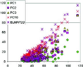
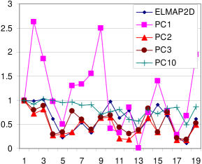
a)                                                 b)

Figure 10: a) Sheppard plot ($\hat{d}_{ij}$ vs $d_{ij}$) for a subset of pair-wise distances selected by NatPCA, calculated for the normal tissue dataset where $\hat{d}_{ij}$ are calculated for dimension reduction by elastic maps (ELMap2D), and linear principal components (PC1-PC5, PC10); distances $\hat{d}_{ij}$ calculated in the internal coordinates of the elastic map (ELMap2D) were scaled such that $\hat{d}_{ij}^{ELMap2D}/d_{ij}=1$ for the first (largest) distance; $\hat{d}_{ij}$ for linear manifolds were taken without re-scaling; b) $\hat{d}_{ij}/d_{ij}$ ratios for the first 20 $NatPCA$ components; the ratios are scaled such that $\hat{d}_{ij}/d_{ij}=1$ for the first (largest) distance

Dimension reduction using projections onto low-dimensional linear manifolds leads to distance contraction, i.e. all the pair-wise distances become smaller than they were in the initial multidimensional space. The structure of big distances is reproduced relatively well since linear principal components are aligned along the directions of the biggest variation. This is demonstrated on Fig. 10, where scatters of $\{d_{ij},\hat{d}_{ij}\}$ (so-called Sheppard plots) and scaled ratios $\hat{d}_{ij}/d_{ij}$ are shown for distances from NatPCA set. One can expect that $k$-dimensional PCA is able to reproduce correctly the first $k$ “natural” principal components, and more if the dimension of the data is less than $k$.

However, preservation of the local structure of small distances is generally not guaranteed, hence it is interesting to measure it. We used a simple test which consists of calculating a set of $k$ neighbors in the “reduced” space for every point, and counting how many of them are also point neighbors in the initial high-dimensional space. The measure of local distance structure preservation is the average ratio of the intersection size of these two sets ($k$ neighbors in the “reduced” and the initial space) over $k$. The unit value would correspond to perfect neighborhood preservation, while a value close to zero corresponds to strong distortions or a situation where distant regions of dataspace are projected in the same region of the low-dimensional manifold. The results are provided in Table 3. The elastic maps perform significantly better than the two-dimensional linear principal manifold in two cases and as well as two-dimensional PCA for Dataset II. To evaluate the significance of this improvement, we made a random test to calculate the local neighborhood preservation measure obtained by a pure random selection of points.

Table 3: Local neighbourhood preservation (defined as an average relative number of neighbours, “preserved” after dimension reduction) for two-dimensional (2D) elastic maps (ELMap) and linear PCA manifolds of dimensions 1-5 and 10 (PC1-PC5, PC10). The last column (RANDOM) corresponds to the value calculated for a random choice of neighbours (10000 permutations are made) which is shown together with its standard deviation

Dataset	ELMap	PC1	PC2	PC3	PC4	PC5	PC10	RANDOM
Breast cancer (k=10)	0.26	0.13	0.20	0.28	0.31	0.38	0.47	0.04 $\pm$ 0.06
Bladder cancer (k=5)	0.53	0.34	0.53	0.61	0.64	0.70	0.80	0.12 $\pm$ 0.14
Normal tissues (k=5)	0.49	0.23	0.33	0.43	0.50	0.54	0.69	0.05 $\pm$ 0.09

Class compactness

Now let us suppose that the points are marked by labels, thus defining classes of points. In the process of dimension reduction, various distortions of the data space are possible. Distant points can be closely projected, distorting the picture of inter and intra-class distances existing in the multidimensional space. In this section we analyze how principal manifolds preserve class distance relations in comparison with linear principal manifolds of various dimensions using a simple test for “class compactness”.

For a class $C$, let us define “class compactness” as an average of a proportion of the points of class $C$ among $k$ neighbors of the point. This average is calculated only over the points from the class $C$.

In Table 4, we provide values of “class compactness” for all datasets with different ab initio classes defined. One can see that there are many examples when two-dimensional principal manifolds perform as well as four- or five-dimensional linear manifolds in putting together the points from the same class. It works particularly well for the collection of normal tissues. There are cases when neither linear nor non-linear low-dimensional manifolds could put together points of the same class and there are a few examples when linear manifolds perform better. In the latter cases (Breast cancer’s A, B, lumA, lumB and “unclassified” classes, bladder cancer T1 class), almost all class compactness values are close to the estimated random values which means that these classes have big intra-class dispersions or are poorly separated from the others. In this case the value of class compactness becomes unstable (look, for example, at the classes A and B of the breast cancer dataset) and depends on random factors which can not be taken into account in this framework.

The closer class compactness is to unity, the easier one can construct a decision function separating this class from the others. However, in the high-dimensional space, due to many degrees of freedom, the “class compactness” might be compromised and become better after appropriate dimension reduction. In Table 4 one can find examples when dimension reduction gives better class compactness in comparison with that calculated in the initial space (breast cancer basal subtype, bladder cancer Grade 2 and T1, T2+ classes). It means that sample classifiers can be regularized by dimension reduction using PCA-like methods.

There are several particular cases (breast cancer basal subtype, bladder cancer T2+, Grade 2 subtypes) when non-linear manifolds give better class compactness than both the multidimensional space and linear principal manifolds of the same dimension. In these cases we can conclude that the dataset in the regions of these classes is naturally “curved” (look, for example, at Fig. 7) and the application of non-linear techniques for classification regularization is an appropriate solution.

We can conclude that non-linear principal manifolds provide systematically better or equal resolution of class separation in comparison with linear manifolds of the same dimension. They perform particularly well when there are many small and relatively compact heterogeneous classes (as in the case of normal tissue collection).

Table 4: “Class compactness” before (ND) and after dimension reduction with use of two-dimensional (2D) elastic maps (ElMap) and linear principal manifolds for 1-5 and 19 principal components (PC1-PC5,PC10). The column “Random” shows a random test when $k$ points are selected by chance (10000 permutations have been made). The number of samples in the class is shown in parentheses (only classes with $>$ 2 samples are shown); “unclas.” stands for unclassified samples

Class	ND	ElMap	PC1	PC2	PC3	PC4	PC5	PC10	Random
Breast cancer (GROUP), k=5
A (193 samples)	0.73	0.67	0.71	0.67	0.68	0.69	0.70	0.70	0.67$\pm$0.27
B (93 samples)	0.31	0.30	0.33	0.29	0.35	0.37	0.38	0.31	0.33$\pm$0.21
Breast cancer (TYPE), k=3
lumA (95)	0.61	0.60	0.64	0.65	0.67	0.72	0.71	0.74	0.33$\pm$0.27
basal (55)	0.88	0.93	0.83	0.86	0.88	0.90	0.88	0.89	0.19$\pm$0.17
unclas. (42)	0.28	0.20	0.27	0.25	0.27	0.27	0.30	0.29	0.15$\pm$0.16
normal (35)	0.68	0.28	0.14	0.19	0.31	0.41	0.41	0.55	0.12$\pm$0.19
errb2 (34)	0.62	0.36	0.24	0.34	0.32	0.32	0.43	0.59	0.12$\pm$0.19
lumB (25)	0.21	0.08	0.20	0.20	0.21	0.25	0.23	0.36	0.09$\pm$0.17
Bladder cancer (TYPE), k=3
Ta (20)	0.85	0.83	0.80	0.85	0.85	0.85	0.85	0.85	0.50$\pm$0.29
T1 (11)	0.58	0.67	0.45	0.69	0.67	0.70	0.67	0.63	0.27$\pm$0.26
T2+ (9)	0.85	0.89	0.11	0.85	0.81	0.89	0.78	0.81	0.22$\pm$0.24
Bladder cancer (GRADE), k=3
Grade 3 (32)	0.94	0.92	0.86	0.83	0.90	0.95	0.94	0.94	0.8$\pm$0.23
Grade 2 (6)	0.5	0.61	0.22	0.39	0.67	0.67	0.67	0.61	0.15$\pm$0.23
Normal tissues (TISSUE), k=2
BRAIN (8)	1.0	1.0	1.0	0.94	1.0	1.0	1.0	1.0	0.08$\pm$0.19
HEART (6)	0.92	0.50	0.17	0.25	0.25	0.25	0.33	0.58	0.06$\pm$0.16
THYROID (6)	0.92	0.67	0.17	0.17	0.25	0.17	0.67	0.75	0.06$\pm$0.17
PROSTATE (5)	1.0	0.8	0.0	0.0	0.1	0.4	0.5	1.0	0.05$\pm$0.16
OVARY (5)	0.7	0.6	0.2	0.1	0.3	0.4	0.5	0.7	0.05$\pm$0.15
LUNG (4)	0.88	0.40	0.5	0.63	0.75	0.63	0.63	0.75	0.04$\pm$0.13
ADRENAL (4)	0.625	0.0	0.0	0.0	0.0	0.25	0.5	0.625	0.04$\pm$0.14
LIVER (4)	0.88	0.88	0.13	0.75	0.75	0.88	0.88	0.88	0.04$\pm$0.14
SALIVARY (4)	1.0	1.0	0.25	0.25	0.50	0.88	1.0	1.0	0.04$\pm$0.14
TONSIL (4)	0.88	0.63	0.0	0.13	0.34	0.75	0.75	0.88	0.04$\pm$0.14
LYMPHNODE (4)	0.75	0.25	0.25	0.25	0.0	0.25	0.25	0.25	0.04$\pm$0.14
FALLOPIAN (4)	0.88	0.50	0.0	0.13	0.25	0.25	0.25	0.75	0.04$\pm$0.14
SPLEEN (3)	0.67	0.50	0.50	0.33	0.33	0.89	0.67	0.83	0.03$\pm$0.12
KIDNEY (3)	1.0	0.33	0.0	0.0	0.33	0.33	0.33	0.67	0.03$\pm$0.12
UTERUS (3)	0.83	0.33	0.0	0.33	0.33	0.33	0.33	0.83	0.03$\pm$0.12
BOWEL (3)	0.17	0.0	0.0	0.0	0.0	0.0	0.0	0.0	0.03$\pm$0.12
ESOPHAGUS (3)	0.67	0.0	0.0	0.0	0.0	0.0	0.0	0.67	0.03$\pm$0.12
COLON (3)	0.33	0.0	0.17	0.0	0.0	0.17	0.17	0.17	0.03$\pm$0.12
STOCMACH (3)	0.5	0.0	0.0	0.0	0.0	0.0	0.0	0.0	0.03$\pm$0.12

7 Discussion

Principal Components Analysis already celebrated its 100th anniversary 4Pearson1901 . Nowadays linear principal manifolds are widely used for dimension reduction, noise filtering and data visualization. Recently, methods for constructing non-linear principal manifolds were proposed, including our elastic maps approach which is based on a physical analogy with elastic membranes. We have developed a general geometric framework for constructing “principal objects” of various dimensions and topologies with the simplest quadratic form of the smoothness penalty, which allows very effective parallel implementations.

Following the metaphor of elasticity (Fig. 3), we introduced two smoothness penalty terms, which are quadratic at the node optimization step. As one can see from (4) they are similar to the sum of squared grid approximations of the first and second derivatives . The $U^{\phi}_{E}$ term penalizes the total length (or area, volume) of the principal manifold and, indirectly, makes the grid regular by penalizing non-equidistant distribution of nodes along the grid. The $U^{\phi}_{R}$ term is a smoothing factor, it penalizes the nonlinearity of the ribs after their embedding into the data space.

Such quadratic penalty allows using standard minimization of quadratic functionals (i.e., solving a system of linear algebraic equations with a sparse matrix), which is considerably more computationally effective than gradient optimization of more complicated cost functions, like the one introduced by Kégl. Moreover, the choice of (4) is the simplest smoothness penalty, which is universally applicable.

Minimization of a positive definite quadratic functional can be provided by the sequential one-dimensional minimization for every space coordinate (cyclic). If for a set of coordinates $\{x_{i}\}_{i\in J}$ terms $x_{i}x_{j}$ ($i,j\in J$, $i\neq j$) do not present in the functional, then for these coordinates the functional can be minimized independently. The quadratic functional we formulate has a sparse structure, it gives us the possibility to use parallel minimization that is expected to be particularly effective in the case of multidimensional data. The application of high-throughput techniques in molecular biology such as DNA microarrays provides such data in large quantities. In the case when $n\gg m$ (the space dimension is much bigger than the number of samples) many existing algorithms for computation of principal manifolds (as GTM 4Bishop1998 ) change their performance. In particular, computing the closest nodes with the formula (7) is no longer the limiting step with most computations being required for finding the new node positions at each iteration.

Our approach is characterized by a universal and flexible way to describe the connection of nodes in the grid. The same algorithm, given an initial definition of the grid, provides construction of principal manifolds with various dimensions and topologies. It is implemented together with many supporting algorithms (interpolation/extrapolation formulas, adaptation strategies, and so on) in several programming languages Elmap ; VidaExpert ; VIMIDA .

One important application of principal manifolds is dimension reduction and data visualization. In this field they compete with multidimensional scaling methods and recently introduced algorithms of dimension reduction, such as the locally linear embedding (LLE) Roweis00 and ISOMAP Tenenbaum00 algorithms. The difference between these two approaches is that the later ones seek new point coordinates directly and do not use any intermediate geometrical objects. This has several advantages, in particular that a) there is a unique solution for the problem (the methods are not iterative in their nature, there is no problem of grid initialization) and b) there is no problem of choosing a good way to project points onto a non-linear manifold. Another advantage is that the methods are not limited by several first dimensions in dimension reduction (it is difficult in practice to manipulate non-linear manifolds of dimension more than three). However, when needed we can overcome this limitation by using an iterative calculation of low-dimensional objects.

A principal manifold can serve as a non-linear low-dimensional screen to project data. The explicit introduction of such an object gives additional benefits to users. First, the manifold approximates the data and can be used itself, without applying projection, to visualize different functions defined in data space (for example, density estimation). Also the manifold as a mediator object, “fixing” the structure of a learning dataset, can be used in visualization of data points that were not used in the learning process, for example, for visualization of dataflow “on the fly”. Constructing manifolds does not use a point-to-point distance matrix, this is particularly useful for datasets with large $n$ when there are considerable memory requirements for storing all pair-wise distances. Also using principal manifolds is expected to be less susceptible to additive noise than the methods based on the local properties of point-to-point distances. To conclude this short comparison, LLE and ISOMAP methods are more suitable if the low-dimensional structure in multidimensional data space is complicated but is expected, and if the data points are situated rather tightly on it. Principal manifolds are more applicable for the visualization of real-life noisy observations, appearing in economics, biology, medicine and other sciences, and for constructing data screens showing not only the data but different related functions defined in data space.

In this paper we demonstrated advantages of using non-linear principal manifolds in visualization of DNA microarrays, data massively generated in biological laboratories. The non-linear approach, compared to linear PCA which is routinely used for analysis of this kind of data, gives better representation of distance structure and class information.

References

- (1) Aizenberg L.: Carleman’s Formulas in Complex Analysis: Theory and Applications. Mathematics and its Applications, 244. Kluwer (1993)
- (2) Banfield, J.D., Raftery, A.E.: Ice floe identification in satellite images using mathematical morphology and clustering about principal curves. Journal of the American Statistical Association 87 (417), 7–16 (1992)
- (3) Bishop, C.M., Svensén, M., and Williams, C.K.I.: GTM: The generative topographic mapping. Neural Computation 10 (1), 215–234 (1998)
- (4) Born, M. and Huang, K.: Dynamical theory of crystal lattices. Oxford University Press (1954)
- (5) Cai, W., Shao, X., and Maigret, B.: Protein-ligand recognition using spherical harmonic molecular surfaces: towards a fast and efficient filter for large virtual throughput screening. J. Mol. Graph. Model. 20 (4), 313–28 (2002)
- (6) Dergachev, V.A., Gorban, A.N., Rossiev, A.A., Karimova, L.M., Kuandykov, E.B., Makarenko, N.G., and Steier, P.: The filling of gaps in geophysical time series by artificial neural networks. Radiocarbon 43 2A, 365–371 (2001)
- (7) Dongarra, J., Lumsdaine, A., Pozo, R., and Remington, K.: A sparse matrix library in C++ for high performance architectures. In: Proceedings of the Second Object Oriented Numerics Conference, 214–218 (1994)
- (8) Dyrskjot, L., Thykjaer, T., Kruhoffer, M. et al.: Identifying distinct classes of bladder carcinoma using microarrays. Nat Genetics 33 (1), 90–96 (2003)
- (9) Durbin, R. and Willshaw, D.: An analogue approach to the traveling salesman problem using an elastic net method. Nature 326 (6114), 689–691 (1987)
-
(10)
Elmap: C++ package available online:
http://www.ihes.fr/zinovyev/vidaexpert/elmap - (11) Erwin, E., Obermayer, K., and Schulten, K.: Self-organizing maps: ordering, convergence properties and energy functions. Biological Cybernetics 67, 47–55 (1992)
- (12) Frećhet, M.: Les élements aléatoires de nature quelconque dans un espace distancié. Ann. Inst. H. Poincaré 10, 215–310 (1948)
- (13) Gorban A.N. (ed.): Methods of neuroinformatics (in Russian). Krasnoyarsk State University Press (1998)
- (14) Gorban, A.N., Karlin, I.V., and Zinovyev, A.Yu.: Invariant grids for reaction kinetics. Physica A 333, 106–154. (2004)
- (15) Gorban, A.N., Karlin, I.V., and Zinovyev, A.Yu.: Constructive methods of invariant manifolds for kinetic problems. Phys. Reports 396 (4-6), 197–403 (2004) Preprint online: http://arxiv.org/abs/cond-mat/0311017.
- (16) Gorban, A.N., Pitenko, A.A., Zinov’ev, A.Y., and Wunsch, D.C.: Vizualization of any data using elastic map method. Smart Engineering System Design 11, 363–368 (2001)
- (17) Gorban, A.N. and Rossiev, A.A.: Neural network iterative method of principal curves for data with gaps. Journal of Computer and System Sciences International 38 (5), 825–831 (1999)
- (18) Gorban, A., Rossiev, A., Makarenko, N., Kuandykov, Y., and Dergachev, V.: Recovering data gaps through neural network methods. International Journal of Geomagnetism and Aeronomy 3 (2), 191–197 (2002)
- (19) Gorban, A.N., Rossiev, A.A., and Wunsch D.C.: Neural network modeling of data with gaps: method of principal curves, Carleman’s formula, and other. The talk was given at the USA–NIS Neurocomputing opportunities workshop, Washington DC, July 1999 (Associated with IJCNN’99).
-
(20)
Gorban, A.N. and Zinovyev, A.Yu.: Visualization of data by method
of elastic maps and its applications in genomics, economics and
sociology. Preprint of Institut des Hautes Etudes Scientiques,
M/01/36, 2001.
http://www.ihes.fr/PREPRINTS/M01/Resu/resu-M01-36.html - (21) Gorban, A.N. and Zinovyev, A.Yu.: Method of elastic maps and its applications in data visualization and data modeling. International Journal of Computing Anticipatory Systems, CHAOS 12, 353–369 (2001)
- (22) Gorban, A.N., Zinovyev, A.Yu., and Pitenko, A.A.: Visualization of data using method of elastic maps (in Russian). Informatsionnie technologii 6, 26–35 (2000)
- (23) Gorban, A.N., Zinovyev, A.Yu., and Pitenko, A.A.: Visualization of data. Method of elastic maps (in Russian). Neurocomputers 4, 19–30 (2002)
- (24) Gorban, A.N., Zinovyev, A.Yu., and Wunsch, D.C.: Application of the method of elastic maps in analysis of genetic texts. In: Proceedings of International Joint Conference on Neural Networks (IJCNN Portland, Oregon, July 20-24) (2003)
- (25) Gorban, A. and Zinovyev, A.: Elastic Principal Graphs and Manifolds and their Practical Applications. Computing 75, 359 –379 (2005)
- (26) Gorban, A.N. Sumner, N.R., and Zinovyev A.Y.: Topological grammars for data approximation. Applied Mathematics Letters 20 (2007) 382- 386 (2006)
- (27) Gusev, A.: Finite element mapping for spring network representations of the mechanics of solids. Phys. Rev. Lett. 93(2), 034302 (2004)
- (28) Hastie, T.: Principal curves and surfaces. PhD Thesis, Stanford University (1984)
- (29) Hastie, T. and Stuetzle, W.: Principal curves. Journal of the American Statistical Association 84 (406), 502–516 (1989)
- (30) Zou, H. and Hastie, T.: Regularization and variable selection via the elastic net. J. R. Statist. Soc. B, 67, Part 2, 301- 320 (2005)
- (31) Kaski, S., Kangas, J., and Kohonen, T.: Bibliography of self-organizing map (SOM) papers: 1981-1997. Neural Computing Surveys, 1, 102–350 (1998)
- (32) Kendall, D.G.: A Survey of the Statistical Theory of Shape. Statistical Science, 4 (2), 87–99 (1989)
- (33) Kohonen, T.: Self-organized formation of topologically correct feature maps. Biological Cybernetics 43, 59–69 (1982)
- (34) Kégl: Principal curves: learning, design, and applications. Ph. D. Thesis, Concordia University, Canada (1999)
- (35) Kégl, B. and Krzyzak, A.: Piecewise linear skeletonization using principal curves. IEEE Transactions on Pattern Analysis and Machine Intelligence 24 (1), 59–74 (2002)
- (36) Kégl, B., Krzyzak, A., Linder, T., and Zeger, K.: A polygonal line algorithm for constructing principal curves. In: Neural Information Processing Systems 1998. MIT Press, 501–507 (1999)
- (37) Kégl, B., Krzyzak, A., Linder, T., and Zeger, K.: Learning and design of principal curves. IEEE Transactions on Pattern Analysis and Machine Intelligence 22(2), 281–297 (2000)
- (38) LeBlanc, M. and Tibshirani R.: Adaptive principal surfaces. Journal of the American Statistical Association 89, 53–64 (1994)
- (39) Leung, Y.F. and Cavalieri, D.: Fundamentals of cDNA microarray data analysis. Trends Genet. 19 (11), 649–659 (2003)
- (40) Mirkin, B.: Clustering for Data Mining: A Data Recovery Approach. Chapman and Hall, Boca Raton (2005)
- (41) Mulier, F. and Cherkassky, V.: Self-organization as an iterative kernel smoothing process. Neural Computation 7, 1165–1177 (1995)
- (42) Oja, M., Kaski, S., and Kohonen, T.: Bibliography of Self-Organizing Map (SOM) Papers: 1998-2001 Addendum. Neural Computing Surveys, 3, 1-156 (2003)
- (43) Pearson K.: On lines and planes of closest fit to systems of points in space. Philosophical Magazine, series 6 (2), 559–572 (1901)
- (44) Perou, C.M., Sorlie, T., Eisen, M.B. et al.: Molecular portraits of human breast tumours. Nature 406 (6797), 747–752 (2000)
- (45) “Principal manifolds for data cartography and dimension reduction”, Leicester, UK, August 2006. A web-page with test microarrays datasets provided for participants of the workshop: http://www.ihes.fr/ zinovyev/princmanif2006
- (46) Ritter, H., Martinetz, T., and Schulten, K.: Neural Computation and Self-Organizing Maps: An Introduction. Addison-Wesley Reading, Massachusetts, 1992.
- (47) H. Ritter. Parametrized self-organizing maps. In Proceedings ICANN’93 International Conference on Artificial Neural Networks Amsterdam, 568–575. Springer (1993)
- (48) Roweis, S. and Saul, L.K.: Nonlinear dimensionality reduction by locally linear embedding. Science 290 (2000), 2323–2326 (2000)
- (49) Sayle, R. and Bissell, A.: RasMol: A Program for fast realistic rendering of molecular structures with shadows. In: Proceedings of the 10th Eurographics UK’92 Conference, University of Edinburgh, Scotland (1992)
- (50) Schölkopf, B., Smola, A. and Müller, K.-R.: Nonlinear component analysis as a kernel eigenvalue problem. Neural Computation 10 (5), 1299–1319 (1998)
- (51) Shyamsundar, R., Kim, Y.H., Higgins, J.P. et al.: A DNA microarray survey of gene expression in normal human tissues. Genome Biology 6 R22 (2005)
- (52) Smola, A.J., Williamson, R.C., Mika, S., and Schölkopf B.: Regularized principal manifolds. EuroCOLT’99, Lecture Notes in Artificial Intelligence 1572, 214-229 (1999)
- (53) Smola, A.J., Mika, S., Schölkopf, B., and Williamson, R.C.: Regularized Principal Manifolds. Journal of Machine Learning Research 1, 179-209 (2001)
- (54) Stanford, D. and Raftery, A.E.: Principal curve clustering with noise. IEEE Transactions on Pattern Analysis and Machine Intelligence 22(6), 601–609 (2000)
- (55) Tenenbaum, J.B., Silva, V. De, and Langford J.C.: A global geometric framework for nonlinear dimensionality reduction. Science 290, 2319–2323 (2000)
- (56) Van Gelder, A. and Wilhelms, J.: Simulation of elastic membranes and soft tissue with triangulated spring meshes. Technical Report: UCSC-CRL-97-12 (1997)
- (57) Verbeek, J.J., Vlassis, N., and Krose, B.: A -segments algorithm for finding principal curves. Technical report (2000) (See also Pattern Recognition Letters, 23 (8), (2002) 1009-1017 (2002))
-
(58)
VidaExpert: Stand-alone application for multidimensional data
visualization, available online:
http://bioinfo.curie.fr/projects/vidaexpert -
(59)
VIMIDA: Java-applet for Visualisation of MultIdimensional DAta, available online:
http://bioinfo-out.curie.fr/projects/vimida - (60) Wang, Y., Klijn, J.G., Zhang, Y., Sieuwerts, A.M., Look, M.P., Yang, F., Talantov, D., Timmermans, M., Meijer-van Gelder, M.E., Yu, J. et al.: Gene-expression profiles to predict distant metastasis of lymph-node-negative primary breast cancer. Lancet 365, 671-679 (2005)
- (61) Xie, H. and Qin, H.: A Physics-based framework for subdivision surface design with automatic rules control. In: Proceedings of the Tenth Pacific Conference on Computer Graphics and Applications (Pacific Graphics 2002), IEEE Press, 304–315 (2002)
- (62) Yin, H.: Data visualisation and manifold mapping using ViSOM. Neural Networks, 15, 1005–1016 (2002)
- (63) Yin, H.: Nonlinear multidimensional data projection and visualisation. In: Lecture Notes in Computer Science, vol. 2690, 377–388 (2003)
- (64) Zinovyev A.: Visualization of Multidimensional Data. Krasnoyarsk State University Press Publ. (2000)
- (65) Zinovyev, A.Yu., Gorban, A.N., and Popova, T.G.: Self-organizing approach for automated gene identification. Open Systems and Information Dynamics 10(4), 321–333 (2003)
- (66) Zinovyev, A.Yu., Pitenko, A.A., and Popova, T.G.: Practical applications of the method of elastic maps (in Russian). Neurocomputers 4, 31–39 (2002)