Abstract

We consider a version of random motion of hard core particles on the semi-lattice $1,\ 2,\ 3,\ldots$, where in each time instant one of three possible events occurs, viz., (a) a randomly chosen particle hops to a free neighboring site, (b) a particle is created at the origin (namely, at site $1$) provided that site $1$ is free and (c) a particle is eliminated at the origin (provided that the site $1$ is occupied). Relations to the BKP equation are explained. Namely, the tau functions of two different BKP hierarchies provide generating functions respectively (I) for transition weights between different particle configurations and (II) for an important object: a normalization function which plays the role of the statistical sum for our non-equilibrium system. As an example we study a model where the hopping rate depends on two parameters ($r$ and $\beta$). For time ${\textsc{t}}\to\infty$ we obtain the asymptotic configuration of particles obtained from the initial empty state (the state without particles) and find an analog of the first order transition at $\beta=1$.

1 Introduction

In the famous paper [1] M.Fisher introduced models of one-dimensional random walk of hard core particles on the lattice. We shall consider a specific version of the models that Fisher called random turn walk models. They describe a motion of particles where at each tick of the clock a randomly chosen walker takes a random step. In both types of models each site may be occupied by only one walker at the same time.

In our case we consider a version of this model where particles move along a semi-line, and where also a particle may be created at the origin.

The model. Consider a set of nodes labelled by positive integers, where each nearest neighbors are linked by a pair of opposite arrows. Let us view the nodes $2,\ 3,\ 4,\dots$ as situated to the right of the origin, the node $1$. An arrow which starts at a node $i$ and ends at a node $j$ (where $j=i\pm 1$) is assigned a weight equal to $e^{-{U}_{j}+{U}_{i}}$. Here ${U}=({U}_{1},{U}_{2},\dots)$ is a set of real numbers.

As an initial state of our dynamical system related to a time ${\textsc{t}}=0$, we place a certain number of hard core particles at nodes (”hard-core” means that each node may be occupied by at most one particle), this initial configuration will be denoted by $\lambda^{(0)}$.

Consider a random motion of the hard-core particles where in each time instant one of three possible events occurs: (a) a randomly chosen particle hops along any of arrows attached to the corresponding node (i.e. either to the left or to the right) provided that target node is free of particles; (b) A particle is created at the origin (namely, at site $1$) provided this site is free; (c) a particle is eliminated at the origin (provided that site $1$ is occupied). We shall refer to configurations as neighboring ones if they differ by an elementary event from the list above.

For instance, the empty configuration is an neighboring one to the configuration shown on figure 1, because the last is obtained by the event (b) from the configuration without particles.

The probability of each elementary (i.e. which occurs in one time instant) event is proportional to a weight (or, a rate) of the event which we assign as follows:
(a) For the hop of a particle along an arrow $i\to j$ (where $j=i\pm 1$) the weight is given by $e^{-{U}_{j}+{U}_{i}}$. The weight $r(j):=e^{-{U}_{j}+{U}_{i}},\;j=2,3,\dots$ will be called (right) hopping rate;
(b) For the birth process the weight is $\frac{1}{\sqrt{2}}e^{-{U}_{1}}$ (this weight will be called birth rate $r(1))$;
(c) For the elimination process the weight is $\frac{1}{\sqrt{2}}e^{{U}_{1}}$.

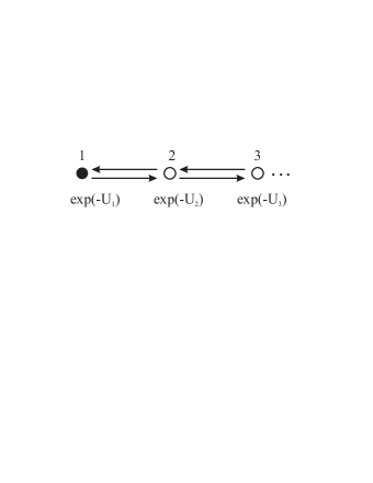
Figure 1: Configuration for ${\textsc{t}}=1$ in case $\lambda^{({\textsc{t}}=0)}$ is the empty configuration. Black ball serves for a particle, white balls for free sites

Along the random process in each each time step, say, ${\textsc{t}}\to{\textsc{t}}+1$ a configuration $\lambda^{({\textsc{t}})}$ goes to a neighboring configuration $\lambda^{({\textsc{t}}+1)}$ with the following probability:

$$p_{\lambda^{({\textsc{t}})}\to\lambda^{({\textsc{t}}+1)}}=\frac{W_{\lambda^{({\textsc{t}})}\to\lambda^{({\textsc{t}}+1)}}}{\sum_{\mu}W_{\lambda^{({\textsc{t}})}\to\mu}}\,,$$ (1)

where $W_{\lambda^{({\textsc{t}})}\to\mu}$ is the weight of the elementary event which creates (in one time step) a configuration $\mu$ from the configuration $\lambda^{({\textsc{t}})}$, the sum in the denominator ranges over all neighboring configurations. For instance, in case the initial configuration is the empty configuration, then by rules (a)-(c) with unit probability we obtain the configuration depicted in figure 1.

Each set of configurations $\lambda^{(0)},\lambda^{(1)},\dots,\lambda^{({\textsc{t}})}$ where each pair $\lambda^{(i)},\lambda^{(i+1)}$ is a pair of neighboring configurations will be referred to as a path of duration t which starts from the configuration $\lambda^{(0)}$ and ends at the configuration $\lambda^{({\textsc{t}})}$. The weight of the path is defined as the product of the weights of all elementary events along the path, $W_{\lambda^{(0)}\to\lambda^{(1)}}W_{\lambda^{(1)}\to\lambda^{(2)}}\cdots W_{\lambda^{({\textsc{t}}-1)}\to\lambda^{({\textsc{t}})}}$. The transition weight between configurations $\lambda^{(0)}$ and $\lambda^{({\textsc{t}})}$ is defined as the sum of weights of all paths of duration t starting from $\lambda^{(0)}$ ending at $\lambda^{({\textsc{t}})}$ and will be denoted by $W_{\lambda^{(0)}\to\lambda^{({\textsc{t}})}}({\textsc{t}})$.

Then, it is easy to see that the probability to come from a configuration $\lambda^{(0)}$ to a given configuration $\lambda^{({\textsc{t}})}$ in t steps is the ratio

$$p_{\lambda^{(0)}\to\lambda^{({\textsc{t}})}}=\frac{W_{\lambda^{(0)}\to\lambda^{({\textsc{t}})}}({\textsc{t}})}{Z_{\lambda^{(0)}}({\textsc{t}})}$$ (2)

where the denominator is a normalization function

$$Z_{\lambda^{(0)}}({\textsc{t}})=\sum_{\mu}W_{\lambda^{(0)}\to\mu}({\textsc{t}})$$ (3)

In what follows we shall omit superscripts for configurations. We shall not need intermediate configurations which were introduced for better explanation of our model.

Our letter is arranged as follows. In an introductory part to section 2 we introduce our tools: neutral fermions and the related Fock space, and quadratic operators (11)-(12) which depends on a given set $U=(U_{1},U_{2},\dots)$. In subsection 2.1 for arbitrary set $U$ we shall obtain an explicit expression for the probability to achieve a given configuration in t steps in case the initial configuration is the empty state (the state without particles), see formulae (27), (34) and (35). For an arbitrary chosen external potential $U$ it is impossible to obtain an asymptotic limit in formulae (34) and (35) in the large time limit. In subsection (2.2) we specify rate $r(n)\;n=1,2,\dots$ by formula (38), now the rate depends on two parameters: a constant denoted by $r$ and an exponent $\beta$. In this case we present the asymptotic formulae for the density of particles, $\sigma(n)$, see (42) and (44). We shall show that for a given and large enough t all characteristics of the asymptotic configuration of particles: its size, the number of involved particles, the center mass e t.c. undergo a jump at $\beta=1$ (when ${\textsc{t}}\to\infty$). We shall show that the normalization function $Z_{\lambda^{(0)}=0}({\textsc{t}})=Z(r,\beta,{\textsc{t}})$ also has a jump. In our problem this function plays a role quite similar to the role of the partition function in statistical physics; in this sense in our model we may treat this jump at $\beta=1$ as a first order phase transition. The expression for probability in different regions of the parameter $\beta$ is given by (55) and (56). Let us note that if we fix $\beta=1$, then, our model turns out to be a discrete time version of the model called asymmetric simple exclusion process (ASEP), now the constant $r$ plays a role of asymmetry parameter. In two parts of subsection 2.3 we shall link respectively transition weights (in item I) and the normalization function (see item II) with tau functions of two different BKP, in the item II the key role is the relation (64) which relates rates $r(n)$ to the BKP higher times.

Let us notice that a wide usage of the free fermion approach to random partitions and certain random processes was presented by Andrei Okounkov in a series of papers, in particular see [2]. Our approach is different and based on (14). It is also different from the approach invented by H.Spohn and K-H.Gwa in [3] for the study of (the continues time) ASEP where spin system was used for the coding of particle configurations. In this approach the state spin up codes the filled stated, spin down the empty state. Via Jordan-Wigner tranform this spin system may be related to fermionic one. However in that case a quadric fermionic Hamiltoinian is used to describe the stochastic dynamics of particles which was identified with Hamiltonian dynamics of quantum spin (or, of nonlinear fermionic) system where the (real) wave function yields the probability distribution for the stochastic process. Following [4] we use free fermions and the answer for the probability is given by the ratio of two factors (35) quite similar to what we have in thermodynamics where the probability of a state is the ratio of the weight of the state and a normalization function (the partition function).

The main part of this work was reported by one of the authors (J.W.L) on the workshop ”Random and integrable models in mathematics and physics” in Brussel, September 11-15, 2007.

2 Fock vectors and configurations of hard core particles

Neutral fermions. In what follows we shall need neutral fermions, $\{\phi_{n}\}_{n\in{\bf Z}}$, as introduced by E. Date, M. Jimbo, M. Kashiwara and T. Miwa in [5], defined by the following property:

$$[\phi_{n},\phi_{m}]_{+}=(-1)^{n}\delta_{n,-m},$$ (4)

where $[\ ,\ ]_{+}$ denotes the anticommutator. In particular, $\left(\phi_{0}\right)^{2}=\frac{1}{2}$. Next we define an action on vacuum states by

$$\phi_{n}|0\rangle=0,\qquad\langle 0|\phi_{-n}=0,\qquad n<0,\qquad\phi_{0}|0\rangle=\frac{1}{\sqrt{2}}|0\rangle,\qquad\langle 0|\phi_{0}=\frac{1}{\sqrt{2}}\langle 0|,$$ (5)

Note that the definition of these ”Fock spaces” is different from the usual one which was introduced in [5]. We follow [6], where the action of $\phi_{0}$ (which is not a number) is different. See Appendix for some more details.

The basis of the corresponding right and left Fock spaces are formed by vectors

$$|\lambda\rangle:=\phi_{\lambda_{1}}\cdots\phi_{\lambda_{N}}|0\rangle$$ (6)

and by

$$\langle\lambda|:=(-1)^{|\lambda|}\langle 0|\phi_{-\lambda_{N}}\cdots\phi_{-\lambda_{1}}\,,$$ (7)

where

$$\lambda_{1}>\cdots>\lambda_{N}>0$$ (8)

and $|\lambda|=\lambda_{1}+\cdots+\lambda_{N}$.

We have one to one correspondence between configurations of hard core particles on the lattice $1,\ 2,\ 3,\dots$ and the basis Fock vectors. These configurations are also called Maya diagrams. Namely, the Maya diagram of the vector $|\lambda\rangle$ is a set of vertices $1,\ 2,\ 3,\dots$, where each vertex numbered by $\lambda_{i}$ is drawn as the black ball (a hard core particle), all other vertices are white balls.

As we see, by (4)-(5) we have

$$\langle\lambda|\mu\rangle=\delta_{\lambda,\mu}$$ (9)

Consider the following operator

$$B=B_{1}(U)+B_{-1}(U)$$ (10)

where $U=(U_{1},U_{2},\dots)$, is a semi-infinite set of numbers (which may be also considered as variables), and where

$$B_{1}(U)=\sum_{i>0}^{\infty}(-1)^{i+1}\phi_{i}\phi_{1-i}e^{-U_{i}+U_{i-1}}=\phi_{1}\phi_{0}e^{-U_{1}}-\phi_{2}\phi_{-1}e^{-U_{2}+U_{1}}+\phi_{3}\phi_{-2}e^{-U_{3}+U_{2}}-\cdots$$ (11)

and

$$B_{-1}(U)=\sum_{i\geq 0}^{\infty}(-1)^{i+1}\phi_{i}\phi_{-1-i}e^{-U_{i}+U_{i+1}}=-\phi_{0}\phi_{-1}e^{U_{1}}+\phi_{1}\phi_{-2}e^{-U_{1}+U_{2}}-\phi_{2}\phi_{-3}e^{-U_{2}+U_{3}}-\cdots$$ (12)

It is straightforward to check the relations

$$B_{-1}B_{1}-B_{1}B_{-1}=\frac{1}{2}\ ,\qquad B_{-1}|0\rangle=0=\langle 0|B_{1}\,,$$ (13)

which we shall need soon for the calculation of (21). At last let us note that for different purpose the operators $B_{1}$ and $B_{-1}$ were used in [7] (namely, to construct examples of multivariable hypergeometric functions which are also multisoliton BKP tau functions [8]).

2.1 Stochastic system: description via fermions

The birth-death of particles at the origin and their diffusive motion may be described as follows.

A sequence of Fock vectors

$$|\lambda^{\prime}\rangle\rightarrow\left(B_{1}(U)+B_{-1}(U)\right)|\lambda^{\prime}\rangle\rightarrow\cdots\rightarrow\left(B_{1}(U)+B_{-1}(U)\right)^{{\textsc{t}}}|\lambda^{\prime}\rangle\rightarrow\cdots$$ (14)

describes an evolution of the initial (basis) Fock vector $|\lambda^{\prime}\rangle$ - where the variable ${\textsc{t}}=0,1,2,\dots$ plays a role of discrete time - to linear combinations of different basis Fock vectors. Due to the correspondence between basis Fock vectors and configurations of hard core particles, this evolution may be interpreted as the random process described in section 1, where each time step is numbered by t. The details will be presented below.

Let us notice that each basis Fock vector

$$|\lambda\rangle:=\phi_{\lambda_{1}}\cdots\phi_{\lambda_{N}}|0\rangle$$ (15)

where $\lambda$ is a strict partition which is $\lambda=(\lambda_{1},\lambda_{2},\dots,\lambda_{N})$, that is in one-to-one correspondence with a configuration of particles, located in the nodes with numbers $\lambda_{1}>\dots>\lambda_{N}>0$. This is the reason, why we have chosen (5) as definition of the Fock space and not the one of [5]. For the Fock space introduced in that article this is not the case.

We are interested in the discrete-time version of this random process which is given by (14), where each time step is numbered by t.

As we see via (4) and (5), the first term in the right hand side of (11) describes the creation of a hard-core particle located at the node number $1$ (the origin) (provided that this node is free). Since $\phi_{0}|0\rangle=\frac{1}{\sqrt{2}}|0\rangle$ we assign the weight $\frac{1}{\sqrt{2}}e^{-U_{1}}$ to this creation process. Each other term of $B_{1}$ describes a hop to the right. Similarly, the first term of $B_{-1}$ in the right hand side of (12) describes the elimination of a particle located at the node $1$ (provided that this node is occupied). Since again $\phi_{0}|0\rangle=\frac{1}{\sqrt{2}}|0\rangle$ we assign the weight $\frac{1}{\sqrt{2}}e^{U_{1}}$ to each elimination process. Other terms of $B_{-1}$ describes the hops to the left (backward motion in the direction of the origin).

It is not difficult to see that

$$W_{\lambda^{\prime}\to\lambda}(U;{\textsc{t}}):=\langle\lambda|\left(B_{1}(U)+B_{-1}(U)\right)^{{\textsc{t}}}|\lambda^{\prime}\rangle$$ (16)

is a sum of weights of paths over all paths of duration t starting at the configuration $\lambda^{\prime}$ and ending at the configuration $\lambda$, and, therefore, yields the transition weight of the t-step random process which describes a transition from an initial configuration of the hard-core particles described by coordinates $\lambda_{1}^{\prime},\dots,\lambda_{N^{\prime}}^{\prime}$ to a target configuration $\lambda_{1},\dots,\lambda_{N}$ defined in the Introduction. As the number of particles does not have to be conserved along the process, $N$ is not necessarily equal to $N^{\prime}$. Let us mark that for each path from a configuration $\lambda^{\prime}$ to a configuration $\lambda$ of a duration t we have

$$N-N^{\prime}=n_{+}-n_{-}$$ (17)

$${\textsc{t}}=j_{+}+j_{-}+n_{+}+n_{-}$$ (18)

$$|\lambda|-|\lambda^{\prime}|=j_{+}-j_{-}+n_{+}-n_{-}$$ (19)

where $j_{+}$ is the number of hops to the left during the time interval t, $j_{-}$ is the number of hops to the right, $n_{+}$ is the number of creations of a particle and $n_{-}$ is the number of eliminations of particles at the node $1$. Let us notice that from (18) and (19) it follows that t and $|\lambda|-|\lambda^{\prime}|$ have the same parity.

Consider the case $\lambda^{\prime}=0$ and look for the weight of the process which transports the initial empty state (there are no particles at all) to a given configuration $\lambda$ in t steps

$$W_{0\to\lambda}(U;{\textsc{t}}):=\langle\lambda|\left(B_{1}(U)+B_{-1}(U)\right)^{{\textsc{t}}}|0\rangle$$ (20)

In order to evaluate the right hand side we need the following formulae

$$e^{z(B_{-1}+B_{1})}=e^{\frac{z^{2}}{4}}e^{zB_{1}}e^{zB_{-1}},\quad e^{zB_{-1}}|0\rangle=|0\rangle\ ,$$ (21)

(the first equation follows from the Baker-Campbell-Hausdorff formula and from (13)), and also the formula

$$\langle\lambda|e^{zB_{1}(U)}|0\rangle=2^{-\frac{N}{2}}z^{|\lambda|}e^{-\sum_{i=1}^{N}U_{\lambda_{i}}}\prod_{i=1}^{N}\frac{1}{\lambda_{i}!}\prod^{N}_{i<j}\frac{\lambda_{i}-\lambda_{j}}{\lambda_{i}+\lambda_{j}}\ ,$$ (22)

see [7],[8]. Here $|\lambda|:=\lambda_{1}+\cdots+\lambda_{N}$ is the weight of $\lambda$. In our case $|\lambda|/N$ is interpreted as the location of the center of mass of the hard core particles.

Now using (21), we obtain

$$\langle\lambda|e^{zB_{1}(U)+zB_{-1}(U)}|0\rangle=e^{\frac{z^{2}}{4}}\langle\lambda|e^{zB_{1}(U)}e^{zB_{-1}(U)}|0\rangle=e^{\frac{z^{2}}{4}}\langle\lambda|e^{zB_{1}(U)}|0\rangle$$ (23)

If we develop the left-hand side and the right-hand side of (23) in powers of the variable $z$, we obtain the following formula for the transition weight from the vacuum state to a state $\lambda$ in a time duration t:

$$\langle\lambda|(B_{1}(U)+B_{-1}(U))^{\textsc{t}}|0\rangle=W_{0\to\lambda}({\textsc{t}})=\frac{{\textsc{t}}!}{m!}\left(\frac{1}{4}\right)^{m}2^{-\frac{N}{2}}e^{-\sum_{i=1}^{N}U_{\lambda_{i}}}\prod_{i=1}^{N}\frac{1}{\lambda_{i}!}\prod^{N}_{i<j}\frac{\lambda_{i}-\lambda_{j}}{\lambda_{i}+\lambda_{j}},$$ (24)

where the right hand side is non-vanishing only if the relation

$${\textsc{t}}=|\lambda|+2m,\quad m=0,1,2,...$$ (25)

is valid. By (18) and (19) we obtain the meaning of $m$, viz.:

$$m=j_{-}+n_{-}$$ (26)

Thus

$$W_{0\to\lambda}(U;{\textsc{t}})=\begin{cases}0&\mbox{ iff }\ {\textsc{t}}-|\lambda|\quad\mbox{odd,}\\ \frac{{\textsc{t}}!}{\left(\frac{{\textsc{t}}-|\lambda|}{2}\right)!}2^{|\lambda|-{\textsc{t}}-\frac{N}{2}}e^{-\sum_{i=1}^{N}U_{\lambda_{i}}}\prod_{i=1}^{N}\frac{1}{\lambda_{i}!}\prod^{N}_{i<j}\frac{\lambda_{i}-\lambda_{j}}{\lambda_{i}+\lambda_{j}}&\mbox{ iff }\ {\textsc{t}}-|\lambda|\quad\mbox{even}\end{cases}$$ (27)

The normalization function, counting weights for all possible target configurations, which may be achieved in the time duration t, is

$$Z(U;{\textsc{t}}):=\sum_{N=0}^{\infty}\sum_{\lambda_{1}>\cdots>\lambda_{N}>0}\langle\lambda|(B_{-1}+B_{1})^{{\textsc{t}}}|0\rangle$$ (28)

$$={\textsc{t}}!\sum_{N=0}^{\infty}2^{-\frac{N}{2}}\sum_{\lambda_{1}>\cdots>\lambda_{N}>0\atop{\textsc{t}}-|\lambda|\;even}\frac{2^{|\lambda|-{\textsc{t}}}}{\Gamma(\frac{{\textsc{t}}-|\lambda|}{2}+1)}\prod_{i=1}^{N}\frac{e^{-U_{\lambda_{i}}}}{\lambda_{i}!}\prod^{N}_{i<j}\frac{\lambda_{i}-\lambda_{j}}{\lambda_{i}+\lambda_{j}}$$ (29)

Note that due to the Gamma function this sum is finite.

The term corresponding to $N=0$ gives in the summation the term $\langle 0|(B_{-1}+B_{1})^{{\textsc{t}}}|0\rangle$.

Let us note that

(1) $|\lambda|=0$ corresponds to the returning to the initial position. This only occurs when the number of time instants is even, ${\textsc{t}}=2m$,

$$W_{0\to 0}({\textsc{t}})=\frac{{\textsc{t}}!}{\left(\frac{{\textsc{t}}}{2}\right)!}2^{-{\textsc{t}}}=2^{-{\frac{{\textsc{t}}}{2}}}({\textsc{t}}-1)!!$$ (30)

(2) Now consider the next case where the final configuration is the one-particle one. Now $\lambda$ is a number which denote the coordinate of this particle. For simplicity we consider $r(n)=r=const$. Then, given large enough t, by Stirling’s formula we can present the transition weight as follows

$$W_{0\to\lambda}=\frac{2^{\lambda-{\textsc{t}}-\frac{1}{2}}}{\lambda!}\frac{{\textsc{t}}!}{\left(\frac{{\textsc{t}}-\lambda}{2}\right)!}e^{-U_{\lambda}}=W_{0\to{\tilde{\lambda}}}\exp\left(-\frac{(\lambda-{\tilde{\lambda}})^{2}}{2\sqrt{{\textsc{t}}}}\right),$$

where

$$\quad W_{0\to{\tilde{\lambda}}}=\frac{{\textsc{t}}!2^{{\tilde{\lambda}}-{\textsc{t}}-\frac{1}{2}}}{\Gamma({\tilde{\lambda}}+1)\Gamma\left(\frac{{\textsc{t}}-{\tilde{\lambda}}}{2}+1\right)}r^{{\tilde{\lambda}}-1}e^{-U_{1}},\quad{\tilde{\lambda}}_{1}=r\sqrt{2{\textsc{t}}}-r^{2}-\frac{1}{2}+O({\textsc{t}}^{-\frac{1}{2}})$$

The formula resembles formula for the Brownian motion (here the variance is given by ${\textsc{t}}^{\frac{1}{4}}$). At last we note, that in case the rate $r$ depends on site, then, in a wide class of rates in large t limit ${\tilde{\lambda}}_{1}$ may be evaluated as the solution of ${\tilde{\lambda}}_{1}=r({\tilde{\lambda}}_{1})\sqrt{2{\textsc{t}}}$. For instance, for Gauss potential, $U_{n}=\frac{1}{2}n^{2}$, one obtains ${\tilde{\lambda}}_{1}\sim\log(2{\textsc{t}})$.

(3) For given $\lambda$ in large t limit (this means that ${\textsc{t}}\gg|\lambda|$) by the Stirling’s approximation we have

$$W_{0\to\lambda}({\textsc{t}})=W_{0\to 0}({\textsc{t}}){\textsc{t}}^{\frac{|\lambda|}{2}}2^{-\frac{N}{2}}e^{-\frac{|\lambda|}{2}}2^{|\lambda|}e^{o({\textsc{t}}^{0})}e^{-E_{\lambda}},$$ (31)

where

$$E_{\lambda}=-\log\;\prod_{i=1}^{N}\frac{e^{-U_{\lambda_{i}}}}{\lambda_{i}!}\prod^{N}_{i<j}\frac{\lambda_{i}-\lambda_{j}}{\lambda_{i}+\lambda_{j}}$$ (32)

means an electrostatic energy of Coulomb particles (placed in an external field) which are attracted by their image. We see that in the large time limit the weight of a configuration increases with $|\lambda|$, and for given t and $|\lambda|$ depends only on the $E_{\lambda}$.

(4) The case ${\textsc{t}}=|\lambda|=n_{+}+j_{+}$ corresponds to the non-stop creation + forward motion processes. Then

$$W_{0\to\lambda}({\textsc{t}})={{\textsc{t}}!}2^{-\frac{N}{2}}e^{-\sum_{i=1}^{N}U_{\lambda_{i}}}\prod_{i=1}^{N}\frac{1}{\lambda_{i}!}\prod^{N}_{i<j}\frac{\lambda_{i}-\lambda_{j}}{\lambda_{i}+\lambda_{j}}$$ (33)

In case the potential is a rapidly decreasing functions $U_{n-1}>>U_{n}$ (and, therefore, left hopping rates are much larger than right hopping rates), then the configurations where ${\textsc{t}}=|\lambda|$ are dominant in the sum for normalization function.

Let us note that up without the factor $2^{-\frac{N}{2}}e^{-\sum_{i=1}^{N}U_{\lambda_{i}}}$ the number $W_{0\to\lambda}({\textsc{t}})$ is equal to the number of shifted standard tableau of shape $\lambda$, see [16], that is the number of ways the Young diagram of the strict partition $\lambda$ may be created by adding box by box to the empty partition in a way that on each step we have the diagram of a strict partition.

Finally, one can get rid of the restriction $\lambda_{1}>\cdots>\lambda_{N}$ in the summation (29) rewriting it as a sum over all non-negative integers $\lambda_{1},\cdots,\lambda_{N}$:

$$Z(U;{\textsc{t}})={{\textsc{t}}}!\sum_{N=0}^{\infty}\frac{2^{-\frac{N}{2}}}{N!}\sum_{\lambda_{1},\cdots,\lambda_{N}>0\atop{\textsc{t}}-|\lambda|\;even}\frac{2^{|\lambda|-{\textsc{t}}}}{\Gamma(\frac{\textsc{t}-|\lambda|}{2}+1)}\prod_{i=1}^{N}\frac{e^{-U_{\lambda_{i}}}}{\lambda_{i}!}\prod^{N}_{i<j}\left|\frac{\lambda_{i}-\lambda_{j}}{\lambda_{i}+\lambda_{j}}\right|$$ (34)

The probability to come to a configuration $\lambda$ in t steps starting from the vacuum one is given by

$$p_{0\to\lambda}(U;{\textsc{t}})=\frac{W_{0\to\lambda}(U;{\textsc{t}})}{Z(U;{\textsc{t}})}$$ (35)

In the present paper we do not write down the expression for the probability $p_{\nu\to\lambda}(U;{\textsc{t}})$ because it is rather cumbersome and contains the so-called skew projective Schur functions.

2.2 Asymptotic configuration of the particles in ${\textsc{t}}\to\infty$ limit

One may ask what configuration is obtained from the empty configuration (vacuum) configuration due to the creation/annihlation processes at the edge of the lattice and to the hops of the particles in the large t limit. (Such configuration will be called asymptotic one and denote as $\lambda({\textsc{t}})$). To find it we should find the largest term in (34). Let us do it via saddle point method. First, in the large t limit it is reasonable to introduce the density of particles $\sigma(u)$, where $u=\frac{\lambda}{R}$ where $R$ is the size of configuration. The number of particles is

$$N=R\int_{0}^{1}\sigma(u)du$$ (36)

Let us note that the density interpolates between full package state ($\sigma(u)=1$), and empty state ($\sigma(u)=0$):

$$0\leq\sigma(u)\leq 1$$ (37)

Let us find the asymptotic configuration in the case when the creation rate is $r(1):=\frac{e^{-U_{1}}}{\sqrt{2}}=r$ and the external potential is

$$U_{n}=-n\log r+(\beta-1)\log n!\;,\quad n=2,3,\dots$$

which means that creation and (the right) hopping rates are as follows

$$r(n)=rn^{1-\beta}\;,\quad n=1,2,3,\dots$$ (38)

$\beta>1$ describes a locking potential while in $\beta<1$ case the potential try to drive particles to the right from the origin. The case $\beta=1$ may be considered as a discrete time version of the so-called asymmetric simple exclusion process (ASEP) on the half-line, now, the parameter $r$ being an asymmetry parameter.

Let notice that formally the point $n=n_{*}=r^{\frac{1}{1-\beta}}$ is a point of an extremum of the potential $U_{n}$ where the left and the right hopping rates are equal.

It means we want to find the configuration $\lambda=\lambda({\textsc{t}})$ where for given t the weight is as follows

$$W_{0\to\lambda}(r,\beta;{\textsc{t}})={\textsc{t}}!\frac{2^{|\lambda|-{\textsc{t}}}}{\left(\frac{{\textsc{t}}-|\lambda|}{2}\right)!}2^{-\frac{N}{2}}e^{-E_{\lambda}(r,\beta)}$$ (39)

here ${\textsc{t}}-|\lambda|$ is even, and the”electrostatic energy“ of the configuration is

$$E_{\lambda}(r,\beta)=\;-\;\log\;\left(r^{|\lambda|}\prod_{i=1}^{N}\frac{1}{(\lambda_{i}!)^{\beta}}\prod^{N}_{i<j}\frac{\lambda_{i}-\lambda_{j}}{\lambda_{i}+\lambda_{j}}\right)$$ (40)

In the continues limit in a standard way one can write the saddle point equation for sum $Z({\textsc{t}})$ which will define the density function $\sigma$ in the large time limit, ${\textsc{t}}\to\infty$. For $\lambda\in(0,R)$ we get

$$\log\frac{r}{\lambda^{\beta}}+P\int_{0}^{R}\frac{\sigma(xR^{-1})dx}{\lambda-x}-P\int_{0}^{R}\frac{\sigma(xR^{-1})dx}{\lambda+x}+\frac{1}{2}\log 2\left({\textsc{t}}-\int_{0}^{R}x\sigma(xR^{-1})dx\right)=0$$ (41)

where $P\int$ stands for the principal value. This equation is to be solved by a standard method [22], see Appendix. For $0<\beta<2$ we find

$$\sigma(\lambda R^{-1})=\frac{\beta}{\pi}\arccos\frac{\lambda}{R},\quad\lambda\in[0,R]$$ (42)

(The validity of (42) may be verified by substitution in (41)). The constraint (37) causes the restriction $0<\beta<2$ for our solution in formula (42).

The weight of such configuration is

$$|\lambda({\textsc{t}})|=R^{2}\int_{0}^{1}u\sigma(u)du=\frac{\beta R^{2}}{8}$$ (43)

and after substitution into the logarithmic term in (41) we obtain a relation of $R$ to t as follows

$${\textsc{t}}=\frac{\beta}{8}R^{2}+\frac{2^{2-2\beta}}{8r^{2}}R^{2\beta}$$ (44)

Let us make a remark. In the approximation we consider one can replace sums by integrals only up to terms of the order $O(R^{0})$. It results to a fact that $r$ in the relation (44) should be replaced by an effective (yet undefined) hopping rate $r_{\mbox{eff}}=r/r_{0}$, where $r_{0}$ is of order $e^{O(R^{0})}$. Below by $r$ we will imply this effective hopping rate. Arguments that $r_{\mbox{eff}}=r$ will be considered separately.

Equation (44) shows that in the large t limit the dependence of $R$ on t is different in regions $0<\beta<1$, $\beta=1$ and $1<\beta<2$. Let us introduce

$$R_{*}=2(\beta r^{2})^{\frac{1}{2(\beta-1)}},\qquad{\textsc{t}}_{*}=\beta(\beta r^{2})^{\frac{1}{\beta-1}}$$

As we see in the region when $R=R_{*}$ the terms in the r.h.s. of (44) are equal. Below we imply that ${\textsc{t}}>>{\textsc{t}}_{*}$. In the large t limit as we see from (44)

$$R=R(\beta,{\textsc{t}})=\begin{cases}\sqrt{\frac{8{\textsc{t}}}{\beta}}&\mbox{ if }\;0<\beta<1\\ \sqrt{\frac{8{\textsc{t}}}{1+r^{-2}}}&\mbox{ if }\;\beta=1\\ 2\left(2r^{2}{\textsc{t}}\right)^{\frac{1}{2\beta}}&\mbox{ if}\;1<\beta<2\end{cases}$$ (45)

Thus, when $0\leq\beta<1$ the size of the asymptotic configuration is proportional to $\sqrt{{\textsc{t}}}$, while in the vicinity of $\beta=2$ we have the forth root behavior. As we see the discontinuity appears at $\beta=1$ in the large t limit. The same behavior has the number of particles in the asymptotic configuration which is proportional to the size of the configuration:

$$N(r,\beta,{\textsc{t}})=R\int_{0}^{1}\left(\frac{\beta}{\pi}\arccos u\right)du=\frac{\beta R(\beta,{\textsc{t}})}{\pi}$$ (46)

The weight of the asymptotic configuration (43) for large enough t is

$$|\lambda({\textsc{t}})|=\frac{\beta R^{2}}{8}\approx\begin{cases}{\textsc{t}}+O\left({\textsc{t}}^{\beta}\right)&\mbox{ if }\ 0<\beta<1\\ \frac{{\textsc{t}}}{1+r^{-2}}&\mbox{ if }\ \beta=1\\ \frac{\beta}{2}\left(2r^{2}{\textsc{t}}\right)^{\frac{1}{\beta}}&\mbox{ if}\ 1<\beta<2\end{cases}$$ (47)

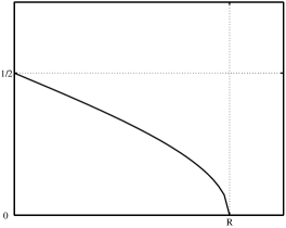
Figure 2: The evolution of the empty configuration in ${\textsc{t}}\to\infty$ limit for $\beta=1$. Asymptotic density of particles.

Notice that the center mass of the configuration also has a jump at $\beta=1$:

$$\frac{|\lambda({\textsc{t}})|}{N(r,\beta,{\textsc{t}})}\approx\begin{cases}\pi\sqrt{\frac{{\textsc{t}}}{8\beta}}&\mbox{ if }\ 0<\beta<1\\ \pi\sqrt{\frac{{\textsc{t}}}{8(1+r^{-2})}}&\mbox{ if }\ \beta=1\\ \frac{\pi}{4}\left(2r^{2}{\textsc{t}}\right)^{\frac{1}{2\beta}}&\mbox{ if}\ 1<\beta<2\end{cases}$$ (48)

For large enough t, the number $m({\textsc{t}})=j_{-}({\textsc{t}})+n_{-}({\textsc{t}})$ depends on region as follows

$$m({\textsc{t}})=\frac{1}{2}({\textsc{t}}-|\lambda|)=\frac{1}{2}{\textsc{t}}-\frac{\beta R^{2}}{16}=\begin{cases}O\left({\textsc{t}}^{\beta}\right)&\mbox{ if }\ 0<\beta<1\\ \frac{{\textsc{t}}}{2(1+r^{2})}&\mbox{ if }\ \beta=1\\ \frac{{\textsc{t}}}{2}-\frac{\beta}{4}\left(2r^{2}{\textsc{t}}\right)^{\frac{1}{\beta}}&\mbox{ if}\ 1<\beta<2\end{cases}$$ (49)

In (47) and (49) we keep terms which we shall use in evaluations below.

For large enough t, the electrostatic energy (40) of $\lambda({\textsc{t}})$ is

$$E_{\lambda({\textsc{t}})}(r,\beta)=-|\lambda({\textsc{t}})|\;\mathrm{ln}\;r\;+$$

$$\left(\beta R^{2}\int_{0}^{1}{\sigma}(u)\left(u\mathrm{ln}(uR)-u\right)du\right)-\frac{1}{2}R^{2}\int_{0}^{1}\int_{0}^{1}{\sigma}(u){\sigma}(u^{\prime})\mathrm{ln}\frac{u-u^{\prime}}{u+u^{\prime}}dudu^{\prime}$$ (50)

$$=|\lambda({\textsc{t}})|\left(\beta\;\mathrm{ln}\;R-\mathrm{ln}\;r\right)-R^{2}\beta^{2}A$$

where

$$\beta^{2}A=-\beta\int_{0}^{1}{\sigma}(u)\left(u\mathrm{ln}u-u\right)du+\int_{0}^{1}du^{\prime}\int_{0}^{u}{\sigma}(u){\sigma}(u^{\prime})\mathrm{ln}\frac{u-u^{\prime}}{u+u^{\prime}}du=\beta^{2}\left(\frac{1}{16}+\frac{\mathrm{ln}\;2}{8}\right)$$ (51)

see Appendix A.4 which yields $A=\frac{1}{16}+\frac{\mathrm{ln}\;2}{8}$.

By (45) and (47) we obtain

$$E_{\lambda({\textsc{t}})}(r,\beta)\approx\begin{cases}\frac{\beta}{2}{\textsc{t}}\mathrm{ln}{\textsc{t}}-{\textsc{t}}\left(\frac{\beta}{2}\mathrm{ln}\frac{\beta}{2}+\frac{\beta}{2}+\mathrm{ln}\;r\right)&\mbox{ if }\ 0<\beta<1\\ \frac{1}{2}\frac{{\textsc{t}}\mathrm{ln}{\textsc{t}}}{1+r^{-2}}+\frac{{\textsc{t}}}{1+r^{-2}}\left(\frac{1}{2}\mathrm{ln}\frac{8}{1+r^{-2}}-8A-\mathrm{ln}\;r\right)&\mbox{ if }\ \beta=1\\ \frac{\beta}{4}\left(2r^{2}{\textsc{t}}\right)^{\frac{1}{\beta}}\left(\mathrm{ln}{\textsc{t}}+(1+2\beta)\mathrm{ln}2-{16}\beta A\right)&\mbox{ if}\;1<\beta<2\end{cases}$$ (52)

Using Stirling’s approximation to evaluate $m({\textsc{t}})!$, for t large, we obtain the weight of the process as follows

$$W_{0\to\lambda({\textsc{t}})}(r,\beta;{\textsc{t}})={\textsc{t}}!\frac{2^{-2m({\textsc{t}})}}{m({\textsc{t}})!}2^{-\frac{N({\textsc{t}})}{2}}e^{-E_{\lambda({\textsc{t}})}(r,\beta)}$$ (53)

$$=\begin{cases}{\textsc{t}}!e^{-\frac{\beta}{2}{\textsc{t}}\mathrm{ln}{\textsc{t}}+{\textsc{t}}\left(\frac{\beta}{2}\mathrm{ln}\frac{\beta}{2}+\frac{\beta}{2}+\mathrm{ln}r\right)+O(\sqrt{{\textsc{t}}})}&\mbox{ if }\ 0<\beta<1\\ {\textsc{t}}!e^{-\frac{{\textsc{t}}}{2}\mathrm{ln}\;{{\textsc{t}}}+{\textsc{t}}\{\frac{\mathrm{ln}\;2(1+r^{2})}{2(1+r^{2})}+\frac{\mathrm{ln}\;2(1+r^{-2})}{2(1+r^{-2})}+\frac{2\mathrm{ln}\;2-1+\mathrm{ln}\;r^{2}}{2(1+r^{-2})}+\frac{1-\mathrm{ln}\;4}{2(1+r^{2})}\}+O(\sqrt{{\textsc{t}}})}&\mbox{ if }\ \beta=1\\ {W_{0\to 0}({\textsc{t}})}e^{-\frac{\beta}{4}\left(2r^{2}{\textsc{t}}\right)^{\frac{1}{\beta}}\left(1-\beta\right)+O\left({\textsc{t}}^{\frac{1}{2\beta}}\right)}&\mbox{if}\;1<\beta<2\end{cases}$$ (54)

Then, as we see the normalization function $Z({\textsc{t}})$ which according to the saddle point method has the same leading term in the large t limit as $W_{0\to\lambda({\textsc{t}})}(r,\beta;{\textsc{t}})$ has a discontuinity at $\beta=1$ which may be interpreted as a sort of the first kind phase transition in our non-equilibrium system.

Now we can evaluate the type of asymptotic of the probability to achieve a given configuration in ${\textsc{t}}\to\infty$ steps. We have $Z({\textsc{t}})=W_{0\to\lambda({\textsc{t}})}({\textsc{t}})e^{O(\mathrm{ln}R)}$, where the last factor originates from the Gaussian integral around the saddle point configuration $\lambda({\textsc{t}})$. Then for ${\textsc{t}}\gg|\lambda|$ we have

$$p_{0\to\lambda}(r,\beta,{\textsc{t}})\approx\frac{W_{0\to\lambda}(r,\beta,{\textsc{t}})}{W_{0\to\lambda({\textsc{t}})}(r,\beta,{\textsc{t}})}\approx{\textsc{t}}^{\frac{|\lambda|}{2}}e^{-\frac{|\lambda|}{2}}2^{|\lambda|}e^{-E_{\lambda}(r,\beta)}e^{\omega({\textsc{t}},r,\beta)}$$ (55)

where $\omega$ does not depend on $\lambda$. (For the enumerator of (55) we used (31) and Stirling’s approximation for (30).)

The answer depends on the region of $\beta$

$$e^{\omega({\textsc{t}},r,\beta)}=\begin{cases}e^{\frac{\beta-1}{2}{\textsc{t}}\mathrm{ln}{\textsc{t}}-{\textsc{t}}\left(\frac{\beta}{2}\mathrm{ln}\frac{\beta}{2}+\frac{\beta}{2}+\mathrm{ln}r)\right)+\frac{{\textsc{t}}}{2}\mathrm{ln}(2e)+O(\sqrt{{\textsc{t}}})}&\mbox{ if }\ 0<\beta<1\\ e^{-{\textsc{t}}\left\{\frac{\mathrm{ln}\;2(1+r^{2})}{2}+\frac{b}{2\left(1+r^{-2}\right)}\right\}+O(\sqrt{{\textsc{t}}})}&\mbox{ if }\ \beta=1\\ e^{\frac{\beta}{4}\left(2r^{2}{\textsc{t}}\right)^{\frac{1}{\beta}}\left(1-\beta\right)+O\left({\textsc{t}}^{\frac{1}{2\beta}}\right)}&\mbox{ if}\;1<\beta<2\end{cases}$$ (56)

where $b=2\mathrm{ln}\;2-1\approx 0.4$. As we see, in each case, in the large t limit $e^{\omega}$ is vanishing.

At last let us note the following. As we see in case of a decreasing potential (or, the same, a increasing rightward hopping rate), $0<\beta<1$, the weight of the asymptotic configuration is equal to t which means that the asymptotic configuration is created by only creating events at the origin and rightward hops, there were no elimination events and backward hops in the history of this configuration, $j_{-}=n_{-}=0$.

For $\beta<0$ solution does not exists. In $\beta\to+0$ limit the number of particles (46) vanishes, while $|\lambda({\textsc{t}})|$ is equal to t. Indeed, the external potential $U_{n}$ is decreasing so rapidly that the largest weight has the one particle configuration where the particle moves in the ballistic way: it is located at the distance t to the origin. When $\beta>2$ we have a locking potential which forces particles to form a sort of a condensate near the origin where all sites are occupied. The size of the condensed phase is defined by $\beta$. This problem is treated by a method similar to the suggested in [21]. Along this way we can show that the solution is given in terms of elliptic integrals of the first and third kind. The problem will be considered in detail in the next version of this paper, where we will show that the normalization function $Z({\textsc{t}})$ has singularity as function of the parameter $\beta$ at $\beta=2$.

2.3 Relation to the BKP tau function

The link of the described stochastic system to integrable equations is two-fold.

(I) A BKP tau function as generating function for transition weights $W_{\lambda^{\prime}\to\lambda}({\textsc{t}})$.

Let us consider the following vacuum expectation value

$$\tau(s,{\bar{s}};U,z):=\langle 0|e^{H(s)}e^{zB}e^{{\bar{H}}({\bar{s}})}|0\rangle$$ (57)

where $B$ is given by (10) and

$$H(s)=\frac{1}{2}\sum_{n=1,3,5,\dots}\sum_{m\in\mathbb{Z}}s_{n}(-1)^{m+1}\phi_{m}\phi_{-n-m},\quad{\bar{H}}({\bar{s}})=\frac{1}{2}\sum_{n=1,3,5,\dots}\sum_{m\in\mathbb{Z}}{\bar{s}}_{n}(-1)^{m+1}\phi_{m}\phi_{n-m}$$ (58)

with $z$, $U=(U_{1},U_{2},\dots)$ and sets $s=(s_{1},s_{3},s_{5}\dots)$ and ${\bar{s}}=({\bar{s}}_{1},{\bar{s}}_{3},{\bar{s}}_{5},\dots)$ parameters. Function $\tau(s,{\bar{s}};U,z)$ depends on $U=(U_{1},U_{2},\dots)$ as the operator $B$ depends on these parameters.

The hierarchy of of Kadomtsev-Petviashvili equations of type B (the BKP hierarchy) was introduced in [5]. As we have already mentioned we use its modification suggested in [6]. These is a semi-infinite set of compatible nonlinear differential equations which may be viewed as a set of commutative time flows. It is common to enumerate the BKP equations (flows) by odd numbers.

Expression (57) where $U$ may be chosen as an arbitrary set of numbers, provides an example of the BKP tau function constructed in [6], where $s=(s_{1},s_{3},s_{5}\dots)$ is the set of the so-called higher times (the times of commutative flows related to different equations of the BKP hierarchy). Actually the set ${\bar{s}}=({\bar{s}}_{1},{\bar{s}}_{3},{\bar{s}}_{5},\dots)$ is also related to a (second) BKP hierarchy of equations, which is compatible with the first one; thus, (57) is an example of the tau function of a coupled BKP hierarchy.

Using results of [9] and doing similar calculations in the framework of BKP hierarchy constructed in [6] (see Appendix) one can show that the operator $e^{H(s)}$ applied to the left vacuum generates all basis left Fock vectors, quite similar $e^{{\bar{H}}({\bar{s}})}$ applied to the right vacuum vector generates all basis right Fock vectors. Namely, we have the following left and right coherent states (see also (6) and (7))

$$\langle 0|e^{H(s)}=\sum_{N=0}^{\infty}2^{-\frac{N}{2}}\sum_{\lambda_{1}>\dots>\lambda_{N}>0}Q_{\lambda}\left(\frac{s}{2}\right)\langle\lambda|\,,$$ (59)

$$e^{{\bar{H}}({s})}|0\rangle=\sum_{N=0}^{\infty}2^{-\frac{N}{2}}\sum_{\lambda_{1}>\dots>\lambda_{N}>0}Q_{\lambda}\left(\frac{s}{2}\right)|\lambda\rangle$$ (60)

where $Q_{\lambda}\left(\frac{s}{2}\right),\;\lambda=(\lambda_{1},\lambda_{2},\dots)$, are known as projective Schur functions, see [16] , which, in an appropriate space, form a complete set of weighted polynomials in the variables $s_{1},s_{3},\dots$. Using these formulae we obtain that the BKP tau function (57) is the generating function for (16), namely

$$\tau(s,{\bar{s}};U,z)=\sum_{{\textsc{t}}=0}^{\infty}\sum_{N,N^{\prime}=0}^{\infty}2^{-\frac{N}{2}-\frac{N^{\prime}}{2}}\sum_{{\lambda_{1}>\dots>\lambda_{N}>0}\atop{\lambda_{1}^{\prime}>\dots>\lambda_{N^{\prime}}^{\prime}>0}}\frac{z^{\textsc{t}}}{{\textsc{t}}!}Q_{\lambda}\left(\frac{s}{2}\right)Q_{\lambda^{\prime}}\left(\frac{\bar{s}}{2}\right)W_{\lambda^{\prime}\to\lambda}(U;{\textsc{t}})$$ (61)

What one obtains in case of a general BKP tau function will be explained in a more detailed forthcoming paper.

(II) A tau function of dual BKP as the generating function for the normalization function $Z({\textsc{t}})$

Let us introduce the generating function for the normalization function (28) as follows

$$Z(U;z):=\sum_{N=0}^{\infty}\sum_{\lambda_{1}>\cdots>\lambda_{N}>0}\langle\lambda|e^{zB}|0\rangle=\sum_{{\textsc{t}}=0}^{\infty}\frac{z^{\textsc{t}}}{{\textsc{t}}!}Z(U;{\textsc{t}})$$ (62)

By (21) and (22) we have

$$Z(U;z)=e^{\frac{z^{2}}{4}}\sum_{N=0}^{\infty}2^{-\frac{N}{2}}\sum_{\lambda_{1}>\cdots>\lambda_{N}>0}z^{|\lambda|}e^{-\sum_{i=1}^{N}U_{\lambda_{i}}}\prod_{i=1}^{N}\frac{1}{\lambda_{i}!}\prod^{N}_{i<j}\frac{\lambda_{i}-\lambda_{j}}{\lambda_{i}+\lambda_{j}}$$

$$=e^{\frac{z^{2}}{4}}\sum_{N=0}^{\infty}\frac{2^{-\frac{N}{2}}}{N!}\sum_{\lambda_{1},\cdots,\lambda_{N}>0}\prod_{i=1}^{N}\frac{e^{\lambda_{i}\mathrm{ln}z-U_{\lambda_{i}}}}{\lambda_{i}!}\prod^{N}_{i<j}\left|\frac{\lambda_{i}-\lambda_{j}}{\lambda_{i}+\lambda_{j}}\right|$$ (63)

Let us mark that the last sum may be compared with the grand partition function of the log Coulomb gas, compare with [18], [19].

Now, we want to present parameters $U=(U_{1},U_{2},\dots)$ as follows

$$U_{n}=-\sum_{m=1,3,5,\dots}^{\infty}n^{m}t_{m}$$ (64)

where $t=(t_{1},t_{3},t_{5},\dots)$ is a new set of parameters (the same parametrization was used in [8]).

Remark 2.1.

Let us notice that our main example (38) is not well fitted into such parametrization. It seems that one needs to introduce an additional flow parameter

$$U_{n}=-\sum_{m=1,3,5,\dots}^{\infty}n^{m}t_{m}+\beta\mathrm{ln}\;n!=-\sum_{m=1,3,5,\dots}^{\infty}n^{m}t_{m}+\beta(n\;\mathrm{ln}\;n-n)$$

and consider the discrete dynamics with respect to $\beta$. In the large t limit we may replace $\mathrm{ln}\;n!$ by $n\;\mathrm{ln}\;n-n$, then it may be related to the flow introduced in in [14].

Then, the right hand side of (63) may be written as the following vacuum expectation value (compare with [11])

$$Z(U;z)=e^{\frac{z^{2}}{4}}\langle 0|e^{H(t)}e^{C(z)}\left(1+\sqrt{2}\sum_{n\geq 0}\frac{z^{n}}{n!}\phi(n)\phi_{0}\right)|0\rangle$$ (65)

$$C(z)=\frac{1}{2}\sum_{n,m\geq 0}\frac{z^{n+m}}{n!m!}\phi(n)\phi(m)sign(m-n),\quad\phi(x):=\sum_{k=-\infty}^{+\infty}x^{k}\phi_{k}$$ (66)

The proof is similar to the proof in [11] its sketch may be found in the Appendix A.5.

Now we notice that (65) is another example of the BKP tau function [6] which may be related to the so-called resonant multi-soliton solution where the number of solitons is infinite and momentum of solitons are nonnegative numbers (compare with [19]). Thus, the tau function of this (dual) BKP hierarchy is a generating function for normalization functions. Via (64), the higher times $t=(t_{1},t_{3},t_{5},\dots)$ of this dual BKP hierarchy parametrize hopping rates of the particles of our stochastic model.

Let us we note that time variables $t=(t_{1},t_{3},t_{5},\dots)$ are integrals of motion for the BKP hierarchy mentioned in (I), in this sense the BKP (II) may be referred as a dual to the BKP (I).

At last let us note that the example (38) where we put $r=e^{t_{1}}$ is related to

$$Z(U;z)=Z(t_{1},\beta;z)=e^{\frac{z^{2}}{4}}\langle 0|e^{H_{1}t_{1}}e^{C(z)}\left(1+\sqrt{2}\sum_{n\geq 0}\frac{z^{n}}{(n!)^{\beta}}\phi(n)\phi_{0}\right)|0\rangle$$

$$C(z)=\frac{1}{2}\sum_{n,m\geq 0}\frac{z^{n+m}}{(n!m!)^{\beta}}\phi(n)\phi(m)sign(m-n),\quad\phi(x):=\sum_{k=-\infty}^{+\infty}x^{k}\phi_{k}$$

One may conjecture that $Z(t_{1},\beta;z)$ is a solution to a difference (with the respect to $\beta$) -differential (with respect to $t_{1}$) Hirota equation.

Discussion

In the continuation of this paper we shall consider our model where the parameter $\beta>2$ describes a model where a condensate of particles (the region of full package) fills a region near the origin. We shall explain the appearance of a phase transition at $\beta=2$ which is rather similar to the transition studied in [21]. The other model where the injection rate is a free parameter will be considered where an analog of the phase transition will be presented, then it may be interesting to discuss links with [15]. It is interesting to understand links with results of [20] and with the approach of [18]. It may be also interesting to link our results with the results of a recent paper [24] where in the context of the quasiclassical limit of Toda lattice hierarchy of integrable equations the Vershik-Kerov limit shape for random partitions was reproduced.

Appendix A Appendices

A.1 A remarks on BKP hierarchies [6] and [5] and related vacuum expectation values

Let us note that different vacuum states were used in the constructions of BKP hierarchy in versions [6] and [5]. If we denote the left and right vacuum states used in [5] respectively by ${}^{\prime}\langle 0|$ and $|0\rangle^{\prime}$ then

$$\langle 0|=\frac{1}{\sqrt{2}}\;{{}^{\prime}\langle 0|}+{{}^{\prime}\langle 0|}\phi_{0},\qquad|0\rangle=\frac{1}{\sqrt{2}}|0\rangle^{\prime}+\phi_{0}|0\rangle^{\prime}$$ (67)

Introduce also

$${}^{\prime}\langle 1|=\sqrt{2}\;^{\prime}\langle 0|\phi_{0},\qquad|1\rangle^{\prime}=\sqrt{2}\phi_{0}|0\rangle^{\prime},$$ (68)

then ${}^{\prime}\langle 0||0\rangle^{\prime}=\,^{\prime}\langle 1||1\rangle^{\prime}=1$ and instead of (5) we have

$$\phi_{n}|0\rangle^{\prime}=\phi_{n}|1\rangle^{\prime}=0,\qquad^{\prime}\langle 0|\phi_{-n}=\,^{\prime}\langle 1|\phi_{-n}=0,\qquad n<0$$ (69)

see [5] for details.

Correspondingly Fock spaces used [6] and [5] are different. From the representational point of view this definition is somewhat more convenient, since each Fock module remains irreducible for the algebra $B_{\infty}$ which is the underlying algebra for KP equations of type B (BKP), see [6].

The vacuum states ${}^{\prime}\langle 0|$ and $|0\rangle^{\prime}$ are more familiar objects in physics. In particular any vacuum expectation value of an odd number of fermions vanishes, while, for instance, $\langle 0|\phi_{0}|0\rangle=\frac{1}{\sqrt{2}}$.

Let $F$ be a product of even number of fermions. Then it is easy to see that

$$\langle 0|F|0\rangle={{}^{\prime}\langle 0|}F{|0\rangle^{\prime}}$$ (70)

Let us note that all vacuum expectation values (v.e.v.) used in the present paper (say, tau functions (57) and (65)) are sums of v.e.v. of monomials containing even number of fermions.

In the context of applications to random process we can construct a model of random motion on the semi-infinite lattice based on the Fock space used in [5], however we find that the Fock space used in [6] is much more natural to our point of view.

A.2 A remark on formulae containing $Q_{\lambda}$ functions

Here we shall show that formulae found in [9] are of use in our case (see also [8]).

From [9] it is known that

$$\begin{split}{{}^{\prime}\langle 0|}e^{H(s)}\phi_{\lambda_{1}}\phi_{\lambda_{2}}\cdots\phi_{\lambda_{N}}|0\rangle^{\prime}=&\begin{cases}2^{-\frac{N}{2}}Q_{(\lambda_{1},{\lambda_{2}},\ldots,{\lambda_{N}})}(\frac{s}{2})\quad&\mbox{for }N\quad\mbox{even},\\ 0&\mbox{for }N\quad\mbox{odd},\end{cases}\\ \sqrt{2}\,{{}^{\prime}\langle 0|}\phi_{0}e^{H(s)}\phi_{\lambda_{1}}\phi_{\lambda_{2}}\cdots\phi_{\lambda_{N}}|0\rangle^{\prime}=&\begin{cases}2^{-\frac{N}{2}}Q_{(\lambda_{1},{\lambda_{2}},\ldots,{\lambda_{N}})}(\frac{s}{2})\quad&\mbox{for }N\quad\mbox{odd},\\ 0&\mbox{for }N\quad\mbox{even},\end{cases}\\ \end{split}$$ (71)

where $Q_{\lambda}\left(\frac{s}{2}\right),\;\lambda=(\lambda_{1},\lambda_{2},\dots)$ are the projective Schur functions, see [16]. Thus

$$\begin{split}&\langle 0|e^{H(s)}\phi_{\lambda_{1}}\phi_{\lambda_{2}}\cdots\phi_{\lambda_{N}}|0\rangle=\\[8.53581pt] &\left(\frac{1}{\sqrt{2}}{{}^{\prime}\langle 0|}+{{}^{\prime}\langle 0|}\phi_{0}\right)e^{H(s)}\phi_{\lambda_{1}}\phi_{\lambda_{2}}\cdots\phi_{\lambda_{N}}\left(\frac{1}{\sqrt{2}}|0\rangle^{\prime}+\phi_{0}|0\rangle^{\prime}\right)=\\[8.53581pt] &\frac{1}{2}\,{{}^{\prime}\langle 0|}e^{H(s)}\phi_{\lambda_{1}}\phi_{\lambda_{2}}\cdots\phi_{\lambda_{N}}|0\rangle^{\prime}+{{}^{\prime}\langle 0|}\phi_{0}e^{H(s)}\phi_{\lambda_{1}}\phi_{\lambda_{2}}\cdots\phi_{\lambda_{N}}\phi_{0}|0\rangle^{\prime}+\\ &+\frac{1}{\sqrt{2}}\,{{}^{\prime}\langle 0|}\phi_{0}e^{H(s)}\phi_{\lambda_{1}}\phi_{\lambda_{2}}\cdots\phi_{\lambda_{N}}|0\rangle^{\prime}+\frac{1}{\sqrt{2}}\,{{}^{\prime}\langle 0|}e^{H(s)}\phi_{\lambda_{1}}\phi_{\lambda_{2}}\cdots\phi_{\lambda_{N}}\phi_{0}|0\rangle^{\prime}\,=\\[8.53581pt] &\frac{1}{2}\,{{}^{\prime}\langle 0|}e^{H(s)}\phi_{\lambda_{1}}\phi_{\lambda_{2}}\cdots\phi_{\lambda_{N}}|0\rangle^{\prime}+\frac{1}{2}\,{{}^{\prime}\langle 1|}e^{H(s)}\phi_{\lambda_{1}}\phi_{\lambda_{2}}\cdots\phi_{\lambda_{N}}|1\rangle^{\prime}+\\ &+\frac{1}{\sqrt{2}}\,{{}^{\prime}\langle 0|}\phi_{0}e^{H(s)}\phi_{\lambda_{1}}\phi_{\lambda_{2}}\cdots\phi_{\lambda_{N}}|0\rangle^{\prime}+\frac{1}{\sqrt{2}}\,{{}^{\prime}\langle 1|}\phi_{0}e^{H(s)}\phi_{\lambda_{1}}\phi_{\lambda_{2}}\cdots\phi_{\lambda_{N}}|1\rangle^{\prime}\,=\\[8.53581pt] &2^{-\frac{N}{2}}Q_{(\lambda_{1},{\lambda_{2}},\ldots,{\lambda_{N}})}\left(\frac{s}{2}\right)\,,\end{split}$$ (72)

since the role of ${{}^{\prime}\langle 0|}$ and ${{}^{\prime}\langle 1|}$ (resp. $|0\rangle^{\prime}$ and $|1\rangle^{\prime}$) is interchangeable.

A.3 Case $0<\beta<2$: Vershik-Kerov type asymptotic

We want to solve the following singular integral equation where $r$ is a given constant:

$$\mathrm{ln}\frac{r}{\lambda^{\beta}}+P\int_{0}^{R}\frac{\sigma(xR^{-1})dx}{\lambda-x}-P\int_{0}^{R}\frac{\sigma(xR^{-1})dx}{\lambda+x}+\frac{1}{2}\mathrm{ln}2\left({\textsc{t}}-\int_{0}^{R}x\sigma(xR^{-1})dx\right)=0$$ (73)

where $\lambda\in[0,R]$ and where $\sigma$ is defined on the interval $x\in[0,R]$. Here and below $P$ serves to denote the principal value of integrals.

Remark A.1.

Let us notice that the second term in (73) describes the repulsion of charges distributed with density $\sigma$ along $(0,R)$, while the third term may be interpreted as the attraction of these charges to their image in the mirror. Then, it is natural to continues $\sigma$ to the interval $(-R,0)$ such that $\sigma(-x):=-\sigma(x)$ (this describes the replacing of particles (with coordinate, say, $x$) by holes (situated in $-x$).

$$P\int_{0}^{R}\frac{\sigma(xR^{-1})dx}{\lambda-x}-P\int_{0}^{R}\frac{\sigma(xR^{-1})dx}{\lambda+x}=P\int_{-R}^{R}\frac{\sigma(xR^{-1})dx}{\lambda-x}$$

Notice that in this case in general we get a jump of $\sigma$ in $x=0$. For our future purpose (of inverting Hilbert type transforms) we prefer to deal with continues functions. For this purpose we shall modify $\sigma$ in the region $(-R,0)$ by adding a constant equal to this jump, $\Delta$, getting continues modified $\sigma$ (compensating this change of $\sigma$ by adding logarithmic term to the right hand side), see below

Now, $\sigma(x)$ is a function defined on the whole interval $[-R,R]$ via relation

$$\sigma(-x)=\Delta-\sigma(x),\quad x\in[-R,R]$$ (74)

(As we shall see later $\Delta=\beta$ if $0<\beta<2$, and $\Delta=2$ if $\beta>2$). Then , we re-write (73) in a more convenient form as

$$P\int_{-R}^{R}\frac{\sigma(xR^{-1})dx}{\lambda-x}=\mathrm{ln}(R+\lambda)^{\Delta}+\mathrm{ln}\lambda^{\beta-\Delta}-\mathrm{ln}(Cr),\quad\lambda\in[-R,R]$$ (75)

where we denoted

$$C^{2}:=2\left({\textsc{t}}-\int_{0}^{R}x\sigma(xR^{-1})dx\right)$$ (76)

$C$ is an independent of $\lambda$ constant to be defined later.

Singular integral equation (75) may be solved by standard method, see [22]. In case $\sigma(xR^{-1})$ is continues and bounded on $[-R,R]$ the solution is given by formulae

$$\sigma(xR^{-1})=-\pi^{-2}P\int_{-R}^{R}\frac{\sqrt{x^{2}-R^{2}}}{\sqrt{\lambda^{2}-R^{2}}}\mathrm{ln}\frac{(\lambda+R)^{\Delta}\lambda^{\delta}}{Cr}\frac{d\lambda}{x-\lambda},\quad x\in[-R,R],$$ (77)

($\delta:=\beta-\Delta$) see formula (42.26) in [22]. Let us evaluate the integral in an explicit way. We consider $\sqrt{\lambda^{2}-R^{2}}$ in the integrand of (77) as single-valued function with the cut $[-R,R]$ whose upper limit on $[-R,R]$ is positive and lower limit on $[-R,R]$ is negative. Also we shall consider $\mathrm{ln}(\lambda+R)^{\Delta}$ in the integrand as the single valued function defined on the whole complex plane with the cut $[-\infty,-R]$. The cut of $\mathrm{ln}\lambda^{\delta}$ will be viewed on the ray $(-\infty,0)$, a little bit above the real axe. Then we have

$$P\int_{-R}^{R}\frac{\sqrt{x^{2}-R^{2}}}{\sqrt{\lambda^{2}-R^{2}}}\mathrm{ln}\frac{(\lambda+R)^{\Delta}\lambda^{\delta}}{Cr}\frac{d\lambda}{x-\lambda}=-\frac{1}{2}\oint_{C}\frac{\sqrt{x^{2}-R^{2}}}{\sqrt{\lambda^{2}-R^{2}}}\mathrm{ln}\frac{(\lambda+R)^{\Delta}\lambda^{\delta}}{Cr}\frac{d\lambda}{x-\lambda}$$ (78)

where the contour $C$ is going crossing the points $0$ and $2R$: $C=-C_{+}+C_{-}$. One can inflate the contour through the point $2R$ as there are no ’bad’ singularities there. We have a cut $(-\infty,0)$ caused by the logarithm. Inflating the contour to the infinity we see that the only contribution will be caused by the cut of the logarithm (we come to the contour which starts on minus infinity going a little bit upper the real line, than turning at the origin and going back to minus infinity a little bit under the real line. (The contribution of the circle embracing infinity vanishes as the integrand’s asymptotic is ${d\lambda\over\lambda^{2}}$.) This yields the integral along the cut

$$P\int_{-R}^{R}\frac{\sqrt{x^{2}-R^{2}}}{\sqrt{\lambda^{2}-R^{2}}}\mathrm{ln}\frac{(\lambda+R)^{\Delta}\lambda^{\delta}}{Cr}\frac{d\lambda}{x-\lambda}=$$ (79)

$$-\frac{1}{2}\int_{-R}^{0}\frac{\sqrt{x^{2}-R^{2}}}{\sqrt{\lambda^{2}-R^{2}}}(2\pi\delta\sqrt{-1})\frac{d\lambda}{x-\lambda}-\frac{1}{2}\int_{-\infty}^{0}\frac{\sqrt{y^{2}-2Ry}}{\sqrt{h^{2}-2Rh}}(2\pi\Delta\sqrt{-1})\frac{dh}{y-h}$$ (80)

where $h=\lambda+R$, $y=x+R$ and $2\pi\Delta\sqrt{-1}$ and $2\pi\Delta\sqrt{-1}$ are the jumps of the logarithm.

The first integral is [23]

$$\int_{-R}^{0}\frac{\sqrt{x^{2}-R^{2}}}{\sqrt{\lambda^{2}-R^{2}}}(2\pi\delta\sqrt{-1})\frac{d\lambda}{x-\lambda}=\arcsin\frac{-R}{2x}$$

As we see taking small $x$ this integral is not a real number; this results in the condition $\delta=0$, or, the same

$$\Delta=\beta$$

For the second integral of (80) we have (see [23]):

$$\int_{0}^{+\infty}\frac{1}{\sqrt{h^{2}+2Rh}}\frac{dh}{y+h}=\frac{1}{\sqrt{-y^{2}+2Ry}}\arccos\left(\frac{y}{R}-1\right)$$ (81)

Inserting the last formula into (80) and then into (77) we finally obtain

$$\sigma(xR^{-1})=\frac{\beta}{\pi}\arccos\frac{x}{R},\quad x\in[0,R],\quad 0\leq\beta\leq 2$$ (82)

We add the last un-equality to provide (37), $0\leq\sigma\leq 1$.

At last let us mark that one may show that if we relate the asymptotic configuration (82) to a strict partition, then, the shape of the Young diagram of the double of this partition will coincide with the so-called Vershik-Kerov asymptotic shape [12],[13].

A.4 Two useful integrals

One can show that

$$\frac{1}{\pi}\int_{0}^{1}\arccos u\;\left(u\mathrm{ln}u-u\right)du=-\frac{1}{8}-\frac{\mathrm{ln}\;2}{8}$$ (83)

$$\frac{1}{\pi^{2}}\int_{0}^{1}du\int_{0}^{u}\arccos u\;\arccos u^{\prime}\;\mathrm{ln}\;\frac{u-u^{\prime}}{u+u^{\prime}}\;du^{\prime}=-\frac{1}{16}$$ (84)

which yields $A=\frac{1}{16}+\frac{\mathrm{ln}\;2}{8}$.

A.5 The relation between formula (65) and (63)

Recal from (66) that $\phi(z)=\sum_{i\in\mathbb{Z}}z^{i}\phi_{i}$. Using (4) and (5), we can also calculate the vacuum expectation value for two of these fields:

$$\begin{split}\langle 0|\phi(z_{1})\phi(z_{2})|0\rangle=&\sum_{m>0}(-z_{2}/z_{1})^{m}+\tfrac{1}{2}\\[8.53581pt] =&\frac{1}{2}\frac{z_{1}-z_{2}}{z_{1}+z_{2}}\,,\end{split}$$ (85)

(where we assume that $|z_{1}|>|z_{2}|$). Using Wick’s Theorem we obtain that

$$\begin{split}\langle 0|\phi(z_{1})\phi(z_{2})\cdots\phi(z_{2m})|0\rangle=&\left(\frac{1}{2}\right)^{m}\prod_{1\leq i<j\leq 2m}\frac{z_{i}-z_{j}}{z_{i}+z_{j}}\,,\\[8.53581pt] \langle 0|\phi(z_{1})\phi(z_{2})\cdots\phi(z_{2m+1})\phi_{0}|0\rangle=&\left(\frac{1}{2}\right)^{m+1}\prod_{1\leq i<j\leq 2m+1}\frac{z_{i}-z_{j}}{z_{i}+z_{j}}\,.\end{split}$$ (86)

For the exponentials of the Hamiltonians $H(t)$ and $\bar{H}(t)$ introduced in (58) one has

$$e^{H(t)}|0\rangle=|0\rangle\qquad\langle 0|e^{\bar{H}(t)}=\langle 0|$$ (87)

and

$$e^{H(t)}\phi(z)e^{-H(t)}=b(t,z)\phi(z),\qquad e^{\bar{H}(t)}\phi(z)e^{-\bar{H}(t)}=b(t,z^{-1})\phi(z),$$ (88)

where

$$b(t,z)=\exp\left(\sum_{n\geq 1,\;\text{odd}}t_{n}z^{n}\right)$$ (89)

Using (86), (87) and (88) we calculate

$$\begin{split}&2^{m}\sum_{{\rm all}\ x_{i}>0}\langle 0|e^{H(t)}\phi(x_{1})\phi(x_{2})\cdots\phi(x_{2m})|0\rangle\prod_{i=1}^{m}sign(x_{2i-1}-x_{2i})\\ =&\sum_{{\rm all}\ x_{i}>0}\prod_{k=1}^{2m}b(t,x_{k})\prod_{1\leq i<j\leq 2m}\frac{x_{i}-x_{j}}{x_{i}+x_{j}}\prod_{i=1}^{m}sign(x_{2i-1}-x_{2i})\\ =&\sum_{\pi\in S_{2m}}\sum_{x_{\pi(2m)}<x_{\pi(2m-1)}<\cdots<x_{\pi(1)}}\prod_{k=1}^{2m}b(t,x_{k})\prod_{1\leq i<j\leq 2m}\frac{x_{i}-x_{j}}{x_{i}+x_{j}}\prod_{i=1}^{m}sign(x_{2i-1}-x_{2i})\\ =&\sum_{\pi\in S_{2m}}\sum_{x_{2m}<x_{2m-1}<\cdots<x_{1}}sign(\pi^{-1})\prod_{k=1}^{2m}b(t,x_{k})\prod_{1\leq i<j\leq 2m}\frac{x_{i}-x_{j}}{x_{i}+x_{j}}\prod_{i=1}^{m}sign(\pi^{-1}(2i)-\pi^{-1}(2i-1))\\ =&2^{m}m!\sum_{x_{2m}<x_{2m-1}<\cdots<x_{1}}\prod_{k=1}^{2m}b(t,x_{k})\prod_{1\leq i<j\leq 2m}\frac{x_{i}-x_{j}}{x_{i}+x_{j}}\\ =&\frac{2^{m}m!}{(2m)!}\sum_{{\rm all}\ x_{i}>0}\prod_{k=1}^{2m}b(t,x_{k})\prod_{1\leq i<j\leq 2m}\left|\frac{x_{i}-x_{j}}{x_{i}+x_{j}}\right|\end{split}$$ (90)

We have used that

$$\sum_{\pi\in S_{2m}}sign(\pi^{-1})\prod_{i=1}^{m}sign(\pi^{-1}(2i)-\pi^{-1}(2i-1))=2^{m}m!$$ (91)

which is obvious if one realizes that the right-hand side of (91) is equal to $2^{m}m!$ times the Pfaffian of the $2m\times 2m$ matrix $A=\left(A_{ij}\right)_{1\leq i,j\leq 2m}$ where $A_{ij}=sign(j-i)$.

Next, we calculate

$$\begin{split}&2^{m+1}\sum_{{\rm all}\ x_{i}>0}\langle 0|e^{H(t)}\phi(x_{1})\phi(x_{2})\cdots\phi(x_{2m})\phi(x_{2m+1})\phi_{0}|0\rangle\prod_{i=1}^{m}sign(x_{2i-1}-x_{2i})\\ =&\sum_{{\rm all}\ x_{i}>0}\prod_{k=1}^{2m+1}b(t,x_{k})\prod_{1\leq i<j\leq 2m+1}\frac{x_{i}-x_{j}}{x_{i}+x_{j}}\prod_{i=1}^{m}sign(x_{2i-1}-x_{2i})\\ =&\sum_{\pi\in S_{2m+1}}\sum_{x_{\pi(2m+1)}<x_{\pi(2m)}<\cdots<x_{\pi(1)}}\prod_{k=1}^{2m+1}b(t,x_{k})\prod_{1\leq i<j\leq 2m+1}\frac{x_{i}-x_{j}}{x_{i}+x_{j}}\prod_{i=1}^{m}sign(x_{2i-1}-x_{2i})\\ =&\sum_{\pi\in S_{2m+1}}\sum_{x_{2m+1}<x_{2m}<\cdots<x_{1}}sign(\pi^{-1})\prod_{k=1}^{2m+1}b(t,x_{k})\prod_{1\leq i<j\leq 2m+1}\frac{x_{i}-x_{j}}{x_{i}+x_{j}}\prod_{i=1}^{m}sign(\pi^{-1}(2i)-\pi^{-1}(2i-1))\\ =&\sum_{\ell=1}^{2m+1}\sum_{\pi\in S_{2m+1},\atop\pi(\ell)=2m+1}\sum_{x_{2m+1}<x_{2m}<\cdots<x_{1}}sign(\pi^{-1})\prod_{k=1}^{2m+1}b(t,x_{k})\prod_{1\leq i<j\leq 2m+1}\frac{x_{i}-x_{j}}{x_{i}+x_{j}}\prod_{i=1}^{m}sign(\pi^{-1}(2i)-\pi^{-1}(2i-1))\\ =&\sum_{\rho\in S_{2m}}\sum_{x_{2m+1}<x_{2m}<\cdots<x_{1}}sign(\rho)\prod_{k=1}^{2m+1}b(t,x_{k})\prod_{1\leq i<j\leq 2m}\frac{x_{i}-x_{j}}{x_{i}+x_{j}}\prod_{i=1}^{m}sign(\rho(2i)-\rho(2i-1))\\ =&2^{m}m!\sum_{x_{2m+1}<x_{2m}<\cdots<x_{1}}\prod_{k=1}^{2m+1}b(t,x_{k})\prod_{1\leq i<j\leq 2m+1}\frac{x_{i}-x_{j}}{x_{i}+x_{j}}\\ =&\frac{2^{m}m!}{(2m+1)!}\sum_{{\rm all}\ x_{i}>0}\prod_{k=1}^{2m+1}b(t,x_{k})\prod_{1\leq i<j\leq 2m+1}\left|\frac{x_{i}-x_{j}}{x_{i}+x_{j}}\right|\end{split}$$ (92)

Here we have used that

$$\begin{split}\sum_{\pi\in S_{2m+1},\atop\pi(\ell)=2m+1}sign(\pi^{-1})\prod_{i=1}^{m}sign(\pi^{-1}(2i)-\pi^{-1}(2i-1))&=\\ -(-)^{\ell}\sum_{\nu\in S_{2m+1},\atop\nu(\ell)=\ell}sign(\nu)\prod_{i=1}^{m}sign(\nu(\epsilon_{\ell}(2i))-\nu(\epsilon_{\ell}(2i-1)))&=\\ -(-)^{\ell}\sum_{\rho\in S_{2m}}sign(\rho)\prod_{i=1}^{m}sign(\rho(2i)-\rho(2i-1))\,,\end{split}$$

where $\epsilon_{\ell}(i)=i$ if $i<\ell$ and $\epsilon_{\ell}(i)=i+1$ if $i>\ell$. So if

$$\pi^{-1}=\begin{pmatrix}1&2&\cdots&\ell-1&\ell&\ell+1&\cdots&2m&2m+1\\ j_{1}&j_{2}&\cdots&j_{\ell-1}&j_{\ell}&j_{\ell+1}&\cdots&j_{2m}&\ell\end{pmatrix}\,,$$

then

$$\nu=\begin{pmatrix}1&2&\cdots&\ell-1&\ell&\ell+1&\ell+2&\cdots&2m&2m+1\\ j_{1}&j_{2}&\cdots&j_{\ell-1}&\ell&j_{\ell}&j_{\ell+1}&\cdots&j_{2m-1}&j_{2m}\end{pmatrix}$$

and

$$\rho=\begin{pmatrix}1&2&\cdots&\ell-1&\ell&\ell+1&\cdots&2m-1&2m\\ i_{1}&i_{2}&\cdots&i_{\ell-1}&i_{\ell}&i_{\ell+1}&\cdots&i_{2m-1}&i_{2m}\end{pmatrix}\,,\quad i_{k}=\begin{cases}j_{k}&{\rm if}\ j_{k}<\ell,\\ j_{k}-1&{\rm if}\ j_{k}>\ell,\end{cases}$$

For instance for $\ell=3$ and $m=2$ one has

$$\pi^{-1}=\begin{pmatrix}1&2&3&4&5\\ 5&1&4&2&3\end{pmatrix}\to\nu=\begin{pmatrix}1&2&3&4&5\\ 5&1&3&4&2\end{pmatrix}\to\rho=\begin{pmatrix}1&2&3&4\\ 4&1&3&2\end{pmatrix}$$

Hence, if we develop (65) as a power series in $z$ and keep the term $e^{\frac{z^{2}}{4}}$. Then substitute (90) and (92) and use (64), we obtain (63).

References

• [1] M. Fisher, “Walks, walls, wetting and melting”, J. Stat. Phys. 34 (1984) 667-729
• [2] A. Okounkov, “Random Matrices and Random Permutations”, arXiv:math-9903176; A. Okounkov, “Infinite wedge and random partitions” arXiv:math-9907127; A. Okounkov, N. Reshetikhin, “Correlation function of Schur process with application to local geometry of a random 3-dimensional Young diagram”, arXiv:math/0107056; A. Okounkov, N. Reshetikhin, “Random skew plane partitions and the Pearcey process”, arXiv:math/0503508
• [3] K-H. Gwa and H. Spohn, “Bethe solution for the dynamical-scaling exponent of the noisy Burgers equation”, Phys. Rev. A 46, 844-854 (1992)
• [4] J. Harnad and A.Yu. Orlov, “Fermionic construction of tau functions and random processes”, Physica D 235 (2007) pp. 168-206
• [5] E. Date, M. Jimbo, M. Kashiwara and T. Miwa, “Transformation groups for soliton equations, IV A new hierarchy of soliton equations of KP-type”, Physica 4D (1982) 343-365
• [6] V. Kac and J. van de Leur, “The Geometry of Spinors and the Multicomponent BKP and DKP Hierarchies”, CRM Proceedings and Lecture Notes 14 (1998) 159-202
• [7] A.Yu. Orlov, “Hypergeometric functions related to Schur Q-polynomials and BKP equation”, Theoretical and Mathematical Physics, 137 (2): 1573-1588 (2003); arXiv:math-ph/0302011
• [8] J.J.C. Nimmo and A.Yu. Orlov, “A relationship between rational and multi-soliton solutions of the BKP hierarchy”, Glasgow Mathematical Journal, 47 A (2005) 149-168; arXiv:nlin/0405009
• [9] Y. You, “Polynomial solutions of the BKP hierarchy and projective representations of symmetric groups”, in Infinite-dimensional Lie algebras and groups, pp. 449-464, Adv. Ser. Math. Phys., 7. World Science Publishing, Teaneck, New Jersey
• [10] J.J.C. Nimmo, “Hall-Littlewood symmetric functions and the BKP equation”. J. Physics A, 23, 751-760 (1990)
• [11] H.Braden, J. Harnad, J.W. van de Leur and A.Yu. Orlov, “Fermionic construction of grand partition function for supersymmetric matrix models and BKP hierarchies”
• [12] A.M.Vershik and S.V.Kerov, “Asymptotics of the Plancherel measure of the symmetric group and the limiting form of Young tableaux”, Soviet Mathematics Doklady 18 (1977) 527-531
• [13] A.M. Vershik and S.V. Kerov, “Asymptotics of the largest and the typical dimensions of the irreducible representations of a symmetric group”, Funktsional’nyi Analiz i Ego Prilozheniya, Vol. 19, No. 1, (1985) pp. 25-36
• [14] T. Eguchi, K. Hori, S.-K. Yang, “Topological $\sigma$-Models and Large-$N$ Matrix Integral”, arXiv:hep-th/9503017
• [15] G.M. Schütz, “Critical phenomena and universal dynamics in one-dimensional driven diffusive systems with two species of particles”, cond-mat/0308450
• [16] I.G. Macdonald, Symmetric Functions and Hall Polynomials, Clarendon Press, Oxford, 1995
• [17] M.L. Mehta, Random Matrices, 2nd edition (Academic, San Diego, 1991).
• [18] P.J. Forrester, “Log Gases and Random Matrices”, book in preparation
http://www.ms.unimelb.edu.au/~​matpjf.matpjf.html
• [19] I.M. Loutsenko and V. Spiridonov, “Soliton Solutions of Integrable Hierarchies and Coulomb Plasmas”, J. Stat. Phys, 99, 751, (2000)
• [20] C. Tracy and H. Widom, “A Limit Theorem for Shifted Schur Measure” math.PR/0210255.
• [21] M.Douglas and V.Kazakov, “Large $N$ phase transitions in continuum $QCD_{2}$ ”, arXiv: hep-th/9305047
• [22] F.D.Gakhov, “Boundary Problems”, ed. 2, Moscow, Nauka 1977
• [23] A.P.Prudnikov, Yu.A.Bychkov and O.I.Marichev “Integrals and Series”, vol I, Moscow, Nauka 1981
• [24] A.Marshakov, “Seiberg-Witten Theory and Extended Toda Hierarchy”, arXiv:hep-th/0712.2802