On the Kinetic Equation and Electrical Resistivity in Systems with Strong Spin- Hole Interaction

Abstract

The problem of constructing the kinetic equation with the description of motion of a hole in systems with strong spin- hole interaction (such as high- temperature superconductors) in terms of the spin polaron has been considered in the framework of the regular antiferromagnetic $s-d$ model. It has been shown by the example of the electrical resistivity that kinetics is determined by the properties of the bands of the spin polaron (rather than ”bar hole”) and their quasiparticle residues $Z_{k}$. The cases of low and optimal doping of the $CuO_{2}$ plane have been considered. It has been shown that the rearrangement of the spectrum of the lower polaron band, as well as the strong doping dependence of the quasiparticle residues $Z_{k}$ is decisive in the unified consideration of these cases.

It is known that the normal state of high- temperature superconductors is characterized by a complex behavior of the spectral and transport properties due to the strong interaction of the carriers with the spin subsystem LeeRMP06 ; DamascelliRMP03 ; Sachdev04+ . This refers to the nontrivial evolution of the hole and spin subsystems with increasing doping, when the system passes from the Mott dielectric to the metallic state Ando04 .

The overwhelming majority of the studies Stojkovic97 on the microscopic description of the kinetics in high- temperature superconductors was devoted to the case of the optimal doping and was based on the concept of the almost antiferromagnetic Fermi liquid described by the spin- fermion Hamiltonian $\hat{H}$ on the square lattice

$$\hat{H}_{t}=\hat{H}+\hat{H}_{f},\quad\hat{H}_{f}=-\widehat{d}^{x}E^{x},$$

$$\hat{H}=\hat{H}_{00}+\widehat{J},\quad\hat{H}_{00}=\hat{H}_{0h}+\hat{I},$$ (1)

$$\hat{H}_{0h}=\sum_{\mathbf{k},\sigma}\varepsilon_{\mathbf{k}}a_{\mathbf{k}\sigma}^{\dagger}a_{\mathbf{k}\sigma},$$

$$\hat{I}=\frac{1}{2}I(1-p)\sum\limits_{\mathbf{R},\mathbf{g}}S_{\mathbf{R+g}}^{\alpha}S_{\mathbf{R}}^{\alpha}+\frac{1}{2}Ip\sum\limits_{\mathbf{R},\mathbf{d}}S_{\mathbf{R+d}}^{\alpha}S_{\mathbf{R}}^{\alpha},$$ (2)

$$\widehat{J}=\frac{J}{\sqrt{N}}\sum\limits_{\mathbf{k},\mathbf{q},\gamma_{1},\gamma_{2}}a_{\mathbf{k}+\mathbf{q},\gamma_{1}}^{\dagger}S_{\mathbf{q}}^{\alpha}\hat{\sigma}_{\gamma_{1}\gamma_{2}}^{\alpha}a_{\mathbf{k}\gamma_{2}}=\sum\limits_{\mathbf{q}}\Lambda_{\mathbf{q}}^{\alpha}S_{\mathbf{q}}^{\alpha},$$

$$\Lambda_{\mathbf{q}}^{\alpha}=\frac{J}{\sqrt{N}}\sum\limits_{\mathbf{k},\gamma_{1},\gamma_{2}}a_{\mathbf{k}+\mathbf{q},\gamma_{1}}^{\dagger}\hat{\sigma}_{\gamma_{1}\gamma_{2}}^{\alpha}a_{\mathbf{k}\gamma_{2}}$$ (3)

The term $\hat{H}_{0h}$ in the Hamiltonian $\hat{H}_{00}$ describes the bar Fermi carriers and contains the spectrum $\varepsilon_{\mathbf{k}}$ of bar holes; $\hat{I}$ corresponds to the frustrated antiferromagnetic interaction between $S=1/2$ spins, $\mathbf{g}$ and $\mathbf{d}$ are the vectors of the first and second neighbors, respectively; and $I_{1}=(1-p)$ and $I_{2}=pI$, where $p$ ($0\leq p\leq 1$) is the frustration parameter, are the respective antiferromagnetic exchange constants. The term $\widehat{J}$ describes the of the the carriers with the subsystem of localized spins $\mathbf{S}_{\mathbf{R}}$ ($\widehat{\sigma}^{\alpha}$ are the Pauli matrices and the summation over repeated Cartesian superscripts $\alpha$ and spin subscripts $\gamma_{1}$ and $\gamma_{2}$ is implied). The total Hamiltonian $\hat{H}_{t}$ includes the interaction $\hat{H}_{f}$ with the electric field $E$, and $\widehat{d}^{x}$ is the dipole momentum operator.

In order to adequately describe the temperature dependence of the electrical resistivity $\rho(T)$ as well as the Hall coefficient $R_{H}(T)$) by solving the kinetic equation in the almost antiferromagnetic liquid model, the spectrum $\varepsilon_{\mathbf{k}}$ in Hamiltonian $\hat{H}_{0h}$ is always changed to the spectrum $E_{\mathbf{k}}^{(1)}$ of the lowest quasiparticle band of the spin polaron, and the operators $a_{\mathbf{k}\sigma}$ in $\hat{H}_{0h}$ are remained fermion operators. The spectrum $E_{\mathbf{k}}^{(1)}$ corresponds to a large Fermi surface and is well measured in experiments on angle resolved photoemission spectroscopy (ARPES). Such a change is not obvious and inevitably leads to the incorrect number of holes $\widetilde{n}_{h}\approx 1.2$ instead of the real relation $n_{h}\lesssim 0.2$. However, for the physical quantities appearing in the kinetic equation and in the expression for the average current, this change seems reasonable, because the kinetic must be determined by the velocities of quasiparticles, $\mathbf{V}_{\mathbf{k}}^{(1)}=\partial E_{\mathbf{k}}^{(1)}/\partial\mathbf{k}$, of the lower polaron band rather than by the velocities of bar holes, $\mathbf{v_{k}}=\partial\varepsilon_{\mathbf{k}}/\partial\mathbf{k}$.

In this study, we present the derivation of the kinetic equation that is based on the Hamiltonian (1) and spin- polaron concept and leads to the observed $\rho(T)$ dependence for the large Fermi surface and $n_{h}\lesssim 0.2$ (due to the small quasiparticle residues $Z_{\mathbf{k}}^{(1)}\lesssim 0.2$ of the lower polaron band in the Green’s function of the bar hole), as well as to the natural appearance of the quasiparticle velocities $\mathbf{V}_{\mathbf{k}}^{(1)}=\partial E_{\mathbf{k}}^{(1)}/\partial\mathbf{k}$.

The carriers are described in the multipole approximation, i.e., in the sufficiently complete basis of the spin polaron. Under the assumption that doping stimulates the frustration of the spin subsystem, the cases of small and optimal doping of the $CuO_{2}$ plane are discussed. The simultaneous consideration of these cases is possible only with allowance for the strong rearrangement of the residue function $Z_{\mathbf{k}}^{(1)}$ with doping.

Let us first consider the equilibrium Green’s functions for bar holes and introduce spin polaron states by an example of the simplest approximation.

At characteristic values $J\simeq 0.1$ eV, the Hamiltonian $\hat{J}$ corresponds to the strong interaction of bar hole with the spin subsystem. As a result, elementary charge excitations must be described by the spin polaron, which is represented as a superposition of the bar- hole operator $a_{\mathbf{k}\sigma}$ and the spin polaron operators describing ”dressing” of the $a_{\mathbf{k}\sigma}$ to the operators of the spin subsystem. The problem is solved with the use of the Mori- Zwanzig projection method for Green’s functions. The method implies the choice of a finite set of the basis operators, which must include the pairing of the bar hole with localized spins from the very beginning.

It is known Bar2001 that the minimum ”good” site set is the following set of the basis operators:

$$\varphi_{\mathbf{r}\sigma}^{(1)}=a_{\mathbf{r}\sigma},\quad\varphi_{\mathbf{r}\sigma}^{(2)}=S^{\alpha}_{\mathbf{r}}\hat{\sigma}^{\alpha}_{\sigma\sigma_{1}}{\,}a_{\mathbf{r}\sigma_{1}},$$ (4)

$$\varphi_{\mathbf{r}\sigma}^{(3)}=\frac{1}{N}\sum\limits_{\mathbf{\rho,q\in\Omega}}{\,}e^{i\mathbf{q\rho}}{\,}S_{\mathbf{r+\rho}}^{\alpha}\hat{\sigma}_{\sigma\sigma_{1}}^{\alpha}{\,}a_{\mathbf{r}\sigma_{1}},$$

$$\varphi_{\mathbf{r}\sigma}^{(4)}=\frac{1}{N}\sum\limits_{\mathbf{\rho,q\in\Omega}}{\,}e^{i\mathbf{q\rho}}{\,}S_{\mathbf{r+\rho}}^{\alpha}\hat{\sigma}_{\sigma\sigma_{1}}^{\alpha}{\,}S_{\mathbf{r}}^{\beta}\hat{\sigma}_{\sigma_{1}\sigma_{2}}^{\beta}{\,}a_{\mathbf{r}\sigma_{2}},$$ (5)

$$\Omega=\{\mathbf{q}:\quad|\pm(\pi/g)-q_{x,y}|<L\}.$$

The first two operators $\varphi_{\mathbf{r}\sigma}^{(1)}$ and $\varphi_{\mathbf{r}\sigma}^{(2)}$ can be treated as local spin- polaron operators, the following two operators $\varphi_{\mathbf{r}\sigma}^{(3)}$ and $\varphi_{\mathbf{r}\sigma}^{(4)}$ correspond to the spin polaron of the intermediate radius and describe the pairing of local polaron operators $\varphi_{\mathbf{r}\sigma}^{(1)}$ and $\varphi_{\mathbf{r}\sigma}^{(2)}$ with the spin wave operators

$$S_{\mathbf{q}}^{\alpha}=\frac{1}{\sqrt{N}}\sum\limits_{\mathbf{\rho}}e^{i\mathbf{q(r+\rho)}}S_{\mathbf{r+\rho}}^{\alpha}.$$

A feature of operators (5) is that they reflect the pairing of spin waves $S_{\mathbf{q}}^{\alpha}$ with momenta $\mathbf{q}$ close to the antiferromagnetic vector $\mathbf{Q}=(\pi,\pi)$, i.e., $\mathbf{q}$ values fill region $\mathbf{\Omega}$ consisting of four $L\times L$ squares in the corners of the first Brillouin zone (in what follow, we set $\Omega=L\times L=0.25(\pi/g)^{2}$). Pairing with such spin waves $S_{\mathbf{q}}^{\alpha}$ takes into account the sharp peak of the spin- spin structure factor in the region close to the antiferromagnetic vector $\mathbf{Q}$ and is responsible for the splitting of the lower quasiparticle band appearing in the local polaron approximation Bar2001 . Moreover, the inclusion of the finite region $\mathbf{\Omega}$ is necessary for describing the correct passage to the limit $T\rightarrow 0$.

The standard projection procedure for solving the equations for Green’s functions in the momentum representation for operators (4) and (5) provides four bands of the spin polaron $E_{\mathbf{k}}^{(s)}$ ($s$ is the band number), an explicit expression for the Green’s function of bar hole, $G_{h}(\mathbf{k},\omega)=\ll a_{\mathbf{k}\sigma}|a_{\mathbf{k}\sigma}^{\dagger}\gg_{\omega}$, the expression for the number of bar holes, $n_{\mathbf{k}\sigma}$ in terms of quasiparticle residues $Z_{\mathbf{k}}^{(l)}$, and makes it possible to represent Hamiltonian $\hat{H}$ given by Eq.(1) in the polaron basis as $\hat{H}_{p}$:

$$G_{h}(\mathbf{k},\omega)={\,}\sum_{s=1}^{4}\frac{Z_{\mathbf{k}}^{(s)}}{\omega-E_{\mathbf{k}}^{(s)}},$$

$$n_{\mathbf{k}\sigma}=\langle a_{\mathbf{k}\sigma}^{\dagger}a_{\mathbf{k}\sigma}\rangle=\sum_{s=1}^{4}Z_{\mathbf{k}}^{(s)}n_{F}(E_{\mathbf{k}}^{(s)});$$ (6)

$$n_{h}=\sum_{\mathbf{k,}\sigma,s}Z_{\mathbf{k}}^{(s)}n_{F}(E_{\mathbf{k}}^{(s)}).$$

Here $n_{F}(E_{\mathbf{k}})=(e^{(E_{\mathbf{k}}-\mu)/T}+1)^{-1}$, where $\mu$ is the chemical potential,

$$\varphi_{\mathbf{k},\sigma}^{(i)}=U_{ij}^{-1}(\mathbf{k})\alpha_{\mathbf{k}\sigma}^{(j)},\quad\langle\langle\alpha_{\mathbf{k}\sigma}^{(s)}|\alpha_{\mathbf{k}\sigma}^{(s^{\prime})\dagger}\rangle\rangle_{\omega}=\frac{1}{\omega-E_{\mathbf{k}}^{(s)}}\delta_{ss^{\prime}},$$

$$Z_{\mathbf{k}}^{(s)}=\overline{U_{s1}^{-1}(\mathbf{k})}U_{s1}^{-1}(\mathbf{k}),\quad u_{\mathbf{k}s}=U_{s1}^{-1}(\mathbf{k}),\quad Z_{\mathbf{k}}^{(s)}=u_{\mathbf{k}s}^{2},$$ (7)

$$\sum\limits_{s}Z_{\mathbf{k}}^{(s)}=1,\quad a_{\mathbf{k},\sigma}=\sum_{s=1}^{4}u_{\mathbf{k}s}\alpha_{\mathbf{k}\sigma}^{(s)},$$

$$\hat{H}_{p}=\sum_{\mathbf{k},\sigma,s}E_{\mathbf{k}}^{(s)}\alpha_{\mathbf{k}\sigma}^{(s)\dagger}\alpha_{\mathbf{k}\sigma}^{(s)}=\hat{H}_{00}+\widehat{J}_{p},$$

$$\widehat{J}_{p}=\widehat{P}\widehat{J}\widehat{P},\quad\widehat{P}=\sum_{\mathbf{k,}s,\gamma}|\alpha_{\mathbf{k,}\gamma}^{(s)}\rangle\langle\alpha_{\mathbf{k,}\gamma}^{\dagger(s)}|$$ (8)

Here, $\widehat{P}$ is the projection operator on the polaron space. The matrix $U_{ij}^{-1}(\mathbf{k})$ is expressed in the explicit form in terms of the spin correlation functions, which are in turn determined in terms of the susceptibility $\chi(\mathbf{q},\omega)$ of the frustrated antiferromagnetic spin subsystem.

The Hamiltonian $\hat{H}_{p}$ contains the operator $\widehat{J}_{p}$, which is a component of $\widehat{J}$ that is responsible for the formation of polaron from a bar hole. Operator $\widehat{J}_{p}$ includes only those matrix elements of $\widehat{J}$ which describe the polaron scattering processes without change in the quasimomentum, i.e., $\widehat{J}_{p}\alpha_{\mathbf{k}\sigma}^{(s1)}\ =>$ $\alpha_{\mathbf{k}\sigma}^{(s2)}$ processes. This scattering processes are taken into account in the projection- approach description of the formation of polarons.

Comparison of the projection- method results for the a complex spin polaron Bar2001 with the self- consistent Born approximation (SCBA) calculations (at $T=0$) Kuzan certainly indicates that the lower band $E_{\mathbf{k}}^{(1)}$ and residues $Z_{\mathbf{k}}^{(1)}$ well reproduce the SCBA peak and its intensity. The upper three bands $E_{\mathbf{k}}^{(2)}$, $E_{\mathbf{k}}^{(3)}$, and $E_{\mathbf{k}}^{(4)}$ effectively describe the incoherent part of $A_{incoh}(\mathbf{k},\omega)$ of the total hole SCBA spectral function

$$A_{SCBA}(\mathbf{k},\omega)=Z_{\mathbf{k}}^{(1)}{\,}\delta(\omega-E_{\mathbf{k}}^{(1)})+A_{incoh}(\mathbf{k},\omega)$$

The motion of the bar hole under the action of, e.g., the external electric field in terms of polaron operators is the motion of spin polaron $\alpha_{\mathbf{k}\sigma}^{(s)}$ simultaneously in four bands with the velocity $\mathbf{V}_{\mathbf{k}}^{(s)}=\partial E_{\mathbf{k}}^{(s)}/\partial\mathbf{k}$.

The operator $\widehat{\widetilde{J}}$ such that $\hat{H}=\hat{H}_{p}+\widehat{\widetilde{J}}$ should be introduced in the kinetic equation. Here, $\widehat{\widetilde{J}}$ should be treated as an operator including the matrix elements of $\widehat{J}$, which lead to polaron- polaron scattering $\widehat{\widetilde{J}}\alpha_{\mathbf{k}\sigma}^{(s1)}$ $=>$ $\alpha_{\mathbf{k+q},\sigma}^{(s2)}S_{\mathbf{-q}}^{\alpha}$ with change in the quasimomentum $\mathbf{q\neq 0}$ and with the simultaneous excitation of the spin subsystem. This vertex obviously must describe the collision term in the kinetic equation for polarons in the second order in $J$.

The Hamiltonian in the polaron representation takes the form (from now on, we take term $\hat{I}$ out of the polaron Hamiltonian $H_{p}$ in explicit way)

$$\hat{H}=\hat{H}_{0}+\widehat{\widetilde{J}},\quad\hat{H}_{0}=\hat{H}_{00}+\widehat{J}_{p}=\hat{H}_{p}+\hat{I}$$ (9)

Here,

$$\hat{H}_{p}=\sum_{\mathbf{k},\sigma,s}E_{\mathbf{k}}^{(s)}\alpha_{\mathbf{k}\sigma}^{(s)\dagger}\alpha_{\mathbf{k}\sigma}^{(s)},$$

where

$$\widehat{\widetilde{J}}=\sum\limits_{\mathbf{q\neq 0,}\alpha}\Lambda_{\mathbf{q}}^{\alpha}S_{\mathbf{q}}^{\alpha},$$

$$\Lambda_{\mathbf{q}}^{\alpha}=\frac{J}{\sqrt{N}}\sum\limits_{\mathbf{k},\gamma_{1},\gamma_{2}}(\sum_{s1=1}^{4}u_{\mathbf{k+q}s1}\alpha_{\mathbf{k+q,}\gamma_{1}}^{\dagger(s1)})\hat{\sigma}_{\gamma_{1}\gamma_{2}}^{\alpha}(\sum_{s2=1}^{4}u_{\mathbf{k}s2}\alpha_{\mathbf{k}\gamma_{2}}^{(s2)}),$$ (10)

$$\hat{H}_{t}=\hat{H}+\hat{H}_{f},\quad\hat{H}_{f}=-\widehat{d}^{x}E,$$

$$\widehat{d}^{x}=e\sum\limits_{\mathbf{k,k^{\prime}},\sigma}x_{\mathbf{kk^{\prime}}}a_{\mathbf{k}\sigma}^{\dagger}a_{\mathbf{k^{\prime}}\sigma},$$ (11)

where

$$x_{\mathbf{kk^{\prime}}}=\langle\mathbf{k}|\hat{x}|\mathbf{k^{\prime}}\rangle=(\Delta_{\mathbf{k}^{{}^{\prime}}\mathbf{,k+q}}+\Delta_{\mathbf{k}^{{}^{\prime}}\mathbf{,k-q}})/2q|_{\lim(q=>0)},$$

$$\mathbf{q}=(q,0);\quad x_{\mathbf{k,k}^{{}^{\prime}}}=x_{\mathbf{k}^{{}^{\prime},}\mathbf{k}}.$$ (12)

The transition to operators $\alpha_{\mathbf{k}\sigma}^{(s)}$ is implied in the operator $\widehat{d}^{x}$ and the quasi- inhomogeneous field $E$ directed along the $X$ axis is introduced according to the Eq. (11).

In order to obtain an expression for the electrical resistivity, we use a variant of the linear- response theory in which the field $E$ that ensures a fixed electrical current $j$ (rather than the current at a fixed field) is sought. Deviation from equilibrium ($\kappa$ is the system deviation parameter specifying $j$) at the initial time $t=0$ is characterized by a finite set of operators $\hat{F}_{l}^{s}$ and the density matrix $\widehat{\widetilde{\rho}}$ is specified in the form

$$\widehat{\widetilde{\rho}}=\hat{\rho}^{0}+\widehat{\phi}^{0},\quad\hat{\rho}^{0}=Z_{0}^{-1}\exp(-\hat{H}_{0}/T),$$

$$\langle\widehat{A}\rangle=Sp\{\hat{\rho}^{0}\widehat{A}\},$$ (13)

$$\widehat{\phi}^{0}=\hat{\rho}^{0}\hat{F},\quad\hat{F}=\sum_{l,s}\eta_{l}^{s}\hat{F}_{l}^{s},$$

$$\langle\hat{F}_{l}^{s}\rangle_{0}=0,\quad\overline{\hat{F}_{l}^{s}}|_{t=0}=\sum_{l_{1},s_{1}}\eta_{l_{1}}^{s_{1}}\langle\hat{F}_{l}^{s}\hat{F}_{l_{1}}^{s_{1}}\rangle,$$ (14)

$$\hat{F}_{l}^{s}=\sum_{\mathbf{k},\sigma}F_{l}^{s}(\mathbf{k)}\alpha_{\mathbf{k}\sigma}^{(s)\dagger}\alpha_{\mathbf{k}\sigma}^{(s)},$$

$$[\hat{F}_{l}^{s},H_{0}]=0,\quad[\hat{F}_{l}^{s},\hat{\rho}^{0}]=0.$$ (15)

Note that the moments $F_{l}^{s}(\mathbf{k)}$ in the current state are odd in $\mathbf{k}$ and the moment $\hat{F}_{1}^{1}=\sum_{\mathbf{k},\sigma}\mathbf{V}_{\mathbf{k}}^{1}\alpha_{\mathbf{k}\sigma}^{(1)\dagger}\alpha_{\mathbf{k}\sigma}^{(1)}$ corresponds to the simplest one- moment approximation associated with the lower polaron band.

The evolution equation for the density matrix $\hat{\rho}_{t}=\widehat{\widetilde{\rho}}+\hat{\rho}_{t}^{\prime}$ has the form $i\frac{\partial\hat{\rho}_{t}^{\prime}}{\partial t}=[(\hat{H}_{0}+\widehat{\widetilde{J}}+\hat{H}_{f}),(\widehat{\widetilde{\rho}}+\hat{\rho}_{t}^{\prime})]$ and its solution for $\hat{\rho}_{t}$ is sought with an accuracy of the first order in $\hat{H}_{f}\sim E\sim\kappa\lambda^{2}$, assuming that $\widehat{\phi}^{0}\sim\kappa$ and $\widehat{\widetilde{J}}\sim\lambda$, where $\lambda$ is the scattering parameter. In this approximation, the transition to the interaction representation [$\widehat{A}(t)=e^{i\hat{H}_{0}t}\widehat{A}e^{-i\hat{H}_{0}t}$] provides

$$\rho_{t}^{\prime}=(-i)\left\{\int_{0}^{t}[H_{f}(\tau-t),\hat{\rho}^{0}]d\tau+\int_{0}^{t}[\widehat{\widetilde{J}}(\tau-t),\widehat{\widetilde{\rho}}]d\tau\right\}$$

$$+(-i)^{2}\int_{0}^{t}d\tau\int_{0}^{\tau}d\tau^{\prime}[\widehat{\widetilde{J}}(\tau-t),[\widehat{\widetilde{J}}(\tau^{\prime}-t),\widehat{\widetilde{\rho}}]].$$ (16)

The conditions of the quasistationarity of the current density matric $\widehat{\widetilde{\rho}}$ in the limit of infinite time reduce to $\overline{\hat{F}_{l}^{s}}|_{t\rightarrow\infty}=\overline{\hat{F}_{l}^{s}}|_{t=0}$, i.e., to the system of equations

$$Sp\{\rho_{t}^{\prime}\hat{F}_{l}^{s}\}|_{t\rightarrow\infty}=0.$$ (17)

In the limit of the infinite number of moments, system (17) is equivalent to the exact kinetic equation for the nonequilibrium one- particle density matrix. The equations of system (17) have the usual kinetic form

$$\left\{i\int_{0}^{t}d\tau Sp\{\hat{F}_{l}^{s}[H_{f}(\tau-t),\hat{\rho}^{0}]\right.$$

$$\left.+\int_{0}^{t}d\tau\int_{0}^{\tau}d\tau^{\prime}Sp\{\hat{F}_{l}^{s}[\widehat{\widetilde{J}}(\tau-t),[\widehat{\widetilde{J}}(\tau^{\prime}-t),\widehat{\phi}^{0}]]\right\}_{t\rightarrow\infty}=0,$$ (18)

where the first and second terms correspond to the field and collision terms, respectively. We denote these terms as $tX_{l}^{s}$ and $tP_{l}^{s}$, respectively. Equations (17) determine coefficients $\eta_{l}^{s}$ in $\widehat{\phi}^{0}$.

The detailed form of the collision term in Eq.(18) includes expression of the form $Sp\{\hat{F}_{l}^{s}\Lambda_{\mathbf{q}_{1}}^{\alpha}(\widetilde{\tau})S_{\mathbf{q}_{1}}^{\alpha}(\widetilde{\tau})\Lambda_{\mathbf{q}_{2}}^{\beta}(\widetilde{\tau}^{\prime})S_{\mathbf{q}_{2}}^{\beta}(\widetilde{\tau}^{\prime})\hat{\rho}^{0}\hat{F}_{l_{1}}^{s_{1}}\}$, where $\widetilde{\tau}=\tau-t$ and $\widetilde{\tau}^{\prime}=\tau-t$, which are calculated with the use of the mode- coupling approximation Plakida97 . In this approximation, ”outer” $S_{\mathbf{q}}^{\alpha}$ operators [i.e., $S_{\mathbf{q}}^{\alpha}$ operators entering into $\widehat{\widetilde{J}}$ in Eqs. (10)] are separately averaged at the first stage and the initial averaging is performed for them. The unaveraged averages of the remaining operators that appear after the above procedure are calculated at the next stage: $Sp{\,}\{\hat{F}_{l}^{s}\Lambda_{\mathbf{q}_{1}}^{\alpha}(\widetilde{\tau})S_{\mathbf{q}_{1}}^{\alpha}(\widetilde{\tau})\Lambda_{\mathbf{q}_{2}}^{\beta}(\widetilde{\tau}^{\prime})S_{\mathbf{q}_{2}}^{\beta}(\widetilde{\tau}^{\prime})\hat{\rho}^{0}\hat{F}_{l_{1}}^{s_{1}}\}$ $=>$ $\left(Sp{\,}\hat{F}_{l}^{s}\Lambda_{\mathbf{q}_{1}}^{\alpha}(\widetilde{\tau})\Lambda_{\mathbf{q}_{2}}^{\beta}(\widetilde{\tau}^{\prime})\hat{\rho}^{0}\hat{F}_{l_{1}}^{s_{1}}\right)\left(Sp{\,}\hat{\rho}^{0}S_{\mathbf{q}_{1}}^{\alpha}(\widetilde{\tau})S_{\mathbf{q}_{2}}^{\beta}(\widetilde{\tau}^{\prime})\right)$

As a result, for the collision term, we obtain

$$P_{l}^{s}=2N{\,}\sum\limits_{l_{1}}\eta_{l_{1}}^{s_{1}}P_{ll_{1}}^{s,s_{1}},$$ (19)

$$P_{ll_{1}}^{s,s_{1}}=J^{2}\frac{1}{N^{2}}{\,}\sum\limits_{\atop{\mathbf{k},\mathbf{q}}{s,s^{\prime}}}\left(F_{l}^{s}(\mathbf{k})-F_{l}^{s}(\mathbf{k+q})\right)$$

$$\times\left(F_{l_{1}}^{s_{1}}(\mathbf{k})-F_{l_{1}}^{s_{1}}(\mathbf{k+q})\right)Z_{\mathbf{k}}^{(s)}Z_{\mathbf{k+q}}^{(s_{1})}$$

$$\times n_{F}(E_{\mathbf{k}}^{(s)})[1-n_{F}(E_{\mathbf{k+q}}^{(s_{1})})]$$

$$\times n_{B}(E_{\mathbf{k+q}}^{(s)}-E_{\mathbf{k}}^{(s_{1})})\chi^{\prime\prime}(\mathbf{q},(E_{\mathbf{k+q}}^{(s_{1})}-E_{\mathbf{k}}^{(s)}))$$ (20)

where $\chi^{\prime\prime}(\mathbf{q},\omega)$ is the imaginary part of spin susceptibility and $n_{B}(\omega)$ is the Bose function.

Under the assumption that $\hat{F}_{l}^{s}$ in the expression for $\widehat{\phi}^{0}$ in Eq. (13) is quasidiagonal, because $H_{f}$ in Eqs. (11) is quasidiagonal, the field term $X_{l}^{s}$ in Eq. (18) is modified to the form

$$X_{l}^{s}=E\sum_{\mathbf{k}}V_{\mathbf{k}}^{x(s)}\left(\frac{-\partial n_{F}(E_{\mathbf{k}}^{(s)})}{\partial E_{\mathbf{k}}^{(1)}}\right)Z_{\mathbf{k}}^{(s)}F_{l}^{s}(\mathbf{k)}.$$ (21)

Finally, the average current is obtained in the form

$$j^{x}=\sum_{l,s}{\,}\eta_{l}^{s}Sp{\,}\{\hat{\rho}\hat{F}_{l}^{s}[\hat{H}_{0},\hat{x}]\}=\frac{2}{g^{2}a_{z}N}$$

$$\times\sum_{l,s,\mathbf{k}}\eta_{l}^{s}F_{l}^{s}(\mathbf{k)}V_{\mathbf{k}}^{x(s)}Z_{\mathbf{k}}^{s}n_{F}(E_{\mathbf{k}}^{(s)})[1-n_{F}(E_{\mathbf{k}}^{(s)})],$$ (22)

where $a_{z}$ is the distance between $CuO_{2}$ planes (we take $a_{z}=6.6$ A and the corresponding volume of the unit cell is $g^{2}a_{z}=93$ A³).

With the use of the coefficients $\eta_{l}^{s}$ obtained from equation $X_{l}^{s}+P_{l}^{s}=0$ (18), the current density and diagonal component of the resistivity tensor $\rho$ can be determined.

For the doping case of interest, $n_{h}\lesssim 0.2$ the chemical potential $\mu$ lies sufficiently deep in the lower polaron band. For this reason, only the lower band $s=1$ can be retained in the expressions for the current and field and collision term; thus, the summation over $s$ is removed in Eqs. (20 and (22. Thus, the problem reduces to a usual one- band case, where the spectrum of the lower polaron band provides the characteristics of the carrier spectrum. The significant difference from traditional expressions is that the residue function $Z_{\mathbf{k}}^{(1)}$ explicitly enters into kinetic equations (20) – (22) and into Eq. (6) for $n_{h}$. Only the lower polaron band will be taken into account and its index 1 will be omitted in the notation of energy, residues, velocities, and coefficients $\eta$ and moments $F_{l}(\mathbf{k)}$ in Eqs. (13).

It is known that the dynamics of charge carriers in $CuO_{2}$ planes is well described by the three- band Emery model Emery87_88 ; Zhang88 . The calculation of the spin polaron spectrum with the use of the Emery model Bar2001 provides the spectrum observed in the ARPES experiments in a wide doping range. The assumption of the correspondence between doping in models with free carriers and frustration $p$ in the pure spin model Inui88 is a key assumption for the description of the properties of the lower polaron band. This assumption is physically natural: a moving hole destroys the magnetic order and the same effect occurs with increasing $p$ in the pure spin model. Moreover, it is based on the similar character of changes in spin correlation functions as functions of $x$ and $p$. However, strict statements on the $x\leftrightarrow p$ correspondence are absent, but frustrations is always present in the spin subsystem at the doped $CuO_{2}$ plane. Even in the dielectric limit, the ratio of exchange on the second neighbors to exchange on on the first neighbors is estimated as $I_{2}/I_{1}\approx 0.1$ Annet89 . The role of frustration as a driving force of the formation of various spin- liquid states is widely discussed. It is expected that a quantum phase transition can occur near $I_{2}/I_{1}\approx 0.5$ (which corresponds to $p\approx 0.3$) LeeRMP06 . Close frustration parameter values are accepted when discussing the stripe scenario of the appearance of incommensurate peaks Sachdev04+ .

A decrease in the spin correlation length $\zeta$ with increasing $p$ corresponds to change in the spin correlation functions, which explicitly appear in the equations for the Green’s functions of the spin polaron and significantly affect the spectrum $E_{\mathbf{k}}$ and residue function $Z_{\mathbf{k}}$. Below, we will discuss the problem of the electrical resistivity for the cases $A$ and $B$ of a small spin correlation length on the order of several lattice constants $\zeta\simeq g$ ($p\simeq 0.3$) and a large spin correlation length $\zeta\gtrsim 10g$ ($p\simeq 0.1$), respectively. Cases $A$ and $B$ refer to cuprates close to optimal doping and to strongly undoped cuprates.

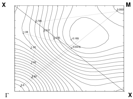
Figure 1: Fig. 1. Hole spectrum $E_{\mathbf{k}}^{A}$ (23) presented by contours $E_{\mathbf{k}}^{A}=const$ in units $\tau=0.2$ $eV$ in the first quarter of the Brillouin zone.

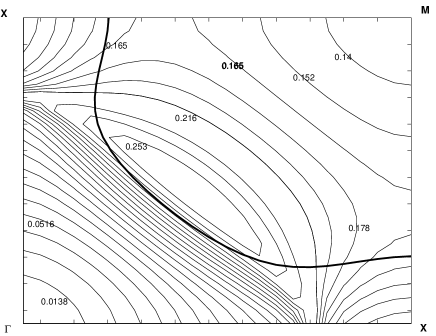
Figure 2: Fig. 2. Residue function $Z_{\mathbf{k}}^{A}$ (doping is close to optimal) presented by contour curves in the first quarter of the Brillouin zone. The thick line is the Fermi surface in case A.

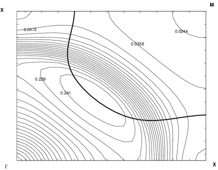
Figure 3: Fig. 3. Residue function $Z_{\mathbf{k}}^{B}$ (low doping) presented by contour curves in the first quarter of the Brillouin zone. The thick line is the Fermi surface in case B.

Spin fermion Hamiltonian (1) applied to the Emery model for case $A$ provides the spectrum $E_{\mathbf{k}}^{A}$ and residue function $Z_{\mathbf{k}}^{A}$ Bar2001 , whose characteristic form is shown in Figs. 1 and 2, respectively. The analytical form of $E_{\mathbf{k}}^{A}$ is approximated with the use of the square- symmetry harmonics

$$E_{\mathbf{k}}^{A}=\tau(a_{1}\gamma_{g}(\mathbf{k})+a_{2}\gamma_{g}^{2}(\mathbf{k})$$

$$+a_{3}\gamma_{d}(\mathbf{k})+a_{4}\gamma_{d}^{2}(\mathbf{k})+a_{5}\gamma_{g}(\mathbf{k})\gamma_{d}(\mathbf{k}));$$ (23)

where

$$\gamma_{g}(\mathbf{k})=(\cos gk_{x}+\cos gk_{y})/2,$$ (24)

$$\gamma_{d}(\mathbf{k})=\cos gk_{x}\cos gk_{y},$$ (25)

and $a_{1}=1.5$, $a_{2}=3.0$, $a_{3}=-1.25$, $a_{4}=0.0$, and $a_{5}=0.1$. The following energy- parameter values characteristic of the Emery model are assumed below: $\tau=0.2$ $eV$, $J=\tau$, $I=0.5\tau$, and temperature $T=0.1I\approx 120$ $K$.

The form of $Z_{\mathbf{k}}^{B}$ is shown in Fig. 3. The form of the spectrum $E_{\mathbf{k}}^{B}$ qualitatively corresponds to the following scenario of the evolution of $E_{\mathbf{k}}$ with increasing $\zeta$: the bottom of the spectrum $E_{\mathbf{k}}^{A}$ (see Fig. 1) is shifted along the $\mathbf{\Gamma}\leftrightarrow\mathbf{M}$ diagonal toward the point $\mathbf{\Gamma}(0,0)$. This shift at low doping ensures a ”large” Fermi surface located near the magnetic Brillouin zone $\mathbf{X}\leftrightarrow\mathbf{X}$. This scenario is confirmed both by ARPES experiments and by calculations of the spin polaron spectrum. In this case, the spectrum $E_{\mathbf{k}}^{B}$ near the Fermi surface and magnetic Brillouin zone is inevitably more flat than the spectrum $E_{\mathbf{k}}^{A}$. This flattering can be treated as the narrowing of the band with increasing the polaron effect (decreasing frustration). In order to taken into account this narrowing, we set $E_{\mathbf{k}}^{B}=0.75{\,}E_{\mathbf{k}}^{A}$. The electrical resistivity is calculated for the Fermi surfaces shown by thick lines in Figs. 2 and 3 for case $A$ ($\mu^{A}=0.82\tau$) and $B$ ($\mu^{B}=0.375\tau$), respectively.

In order to explicitly clarify the role of the flattering of $E_{\mathbf{k}}$ and the $\mathbf{k}$ dependence of $Z_{\mathbf{k}}$, we use the following spin susceptibility for both cases

$$\chi(\mathbf{q},\omega)=\frac{-A_{\mathbf{q}}}{\omega^{2}-\omega_{\mathbf{q}}^{2}+i\omega\gamma}.$$ (26)

This form of the spin susceptibility appears in the framework of the spherically symmetric self- consistent approach Shimahara91 ; BarBerez94-both in the method of irreducible two- time retarded Green’s functions $\langle\langle S_{\mathbf{q}}^{\alpha}|S_{\mathbf{-q}}^{\alpha}\rangle\rangle_{\omega+i\epsilon}$ Tserkovnikov71 ; Plakida73 , BarBerez94-both or in the memory function method Prelovsek04 . The spin susceptibility is taken in the same form as in the case of the calculation of the electrical resistivity at $T=0.1I$ in Bar2007 , where the method of self- consistent calculation of $\chi(\mathbf{q},\omega)$ and choice of damping $\gamma=0.45I$ were discussed in detail.

To take into account strong scattering anisotropy due to the strong scattering of carriers from the spin mode with the antiferromagnetic vector $\mathbf{Q}$, it is inevitably necessary to go beyond the framework of the traditional one moment approximation when solving the kinetic equation. The large number of moments is also necessary for demonstration of the convergence of the method.

Polynomials of the velocity components $V\mathbf{{}_{k}^{\alpha}}$ and their derivatives will be used below as the moments $F_{l}(\mathbf{k})$ of the distribution function:

$$F_{l}^{E}(\mathbf{k})=\{V_{\mathbf{k}}^{x},{\,}(V_{\mathbf{k}}^{y})^{2}V_{\mathbf{k}}^{x},{\,}\frac{\partial V_{\mathbf{k}}^{x}}{\partial k^{y}}V_{\mathbf{k}}^{y},{\,}$$

$$\frac{\partial V_{\mathbf{k}}^{y}}{\partial k^{y}}V_{\mathbf{k}}^{x},{\,}\frac{\partial V_{\mathbf{k}}^{x}}{\partial k^{x}}\frac{\partial V_{\mathbf{k}}^{y}}{\partial k^{y}}V_{\mathbf{k}}^{x},{\,}(V_{\mathbf{k}}^{x})^{3}{\,}\frac{\partial V_{\mathbf{k}}^{x}}{\partial k^{x}}V_{\mathbf{k}}^{x}\}.$$ (27)

For good convergence, it is sufficient to take into account first three or four moments.

Calculations for case $A$ give the electrical resistivity $\rho_{A}=$ $85.2$ $\mu\Omega cm$ and the number of holes $n_{h}=0.21$. This value is comparable with $\rho(T=120K)\approx$ $100$ $\mu\Omega cm$ for $La_{2-x}Sr_{x}CuO_{4}$ with $0.16<x<0.22$ Ando04 . The electrical resistivity $\rho_{A}$ calculated under the assumption $Z_{\mathbf{k}}^{A}=1$ is denoted as $\widetilde{\rho}_{A}$ (below, all the quantities calculated under the assumption $Z_{\mathbf{k}}^{A}=1$ are marked by tilde) and is $\widetilde{\rho}_{A}=84.2\mu\Omega cm\approx\rho_{A}$ and $\widetilde{n}_{h}\approx 1.13$. The values $\widetilde{\rho}_{A}$ and $\rho_{A}$ are approximately equal to each other, because $Z_{\mathbf{k}}^{A}$ depends only slightly on $\mathbf{k}$ in the $\mathbf{k}$- space Brillouin- zone region that it is near the Fermi surface and contributes to kinetics. In this region, $Z_{\mathbf{k}}\approx$ $const=Z$. In this case, $\eta_{l}\sim Z^{-1}$ according Eqs. (19)- (21) and the resistivity $\rho$ determined by the current (22) is independent of $Z$. In this case, the results obtained in the spin- fermion models, where the residue function is disregarded, are valid. However, the smallness of $Z_{\mathbf{k}}^{A}$ ($Z_{\mathbf{k}}^{A}$ $\lesssim 0.2$), as well as the $\mathbf{k}$ dependence of $Z_{\mathbf{k}}$ in the entire $\mathbf{k}$- space Brillouin zone, see Fig. 2, obviously leads to the relation $n_{h}\lesssim 0.2$ at a large Fermi surface and affects the position of the Fermi surface with respect to the magnetic Brillouin zone. The last effect significantly determines the collision integral for strong scattering by the antiferromagnetic vector $\mathbf{Q}$.

In case $B$, $Z_{\mathbf{k}}^{B}$ and the Fermi surface shown in Fig. 3 correctly represent the properties of the spectrum of underdoped cuprates: the hole residues $Z_{\mathbf{k}}^{B}$ decreases from 0.24 to 0.04 when moving along the Fermi surface from the point of intersection with the $\mathbf{-M}$ to thre point of intersection of the Fermi surface with the boundary $\mathbf{X-M}$ of the Brillouin. This decrease qualitatively reflects the known opening of the pseudogap on the Fermi surface. Calculations for the case $B$ lead to $\rho_{B}=$ $231.1$ $\mu\Omega cm$ and the number of holes $n_{h}=0.08$, which is close to $\rho(T=120K)\approx$ $220$ $\mu\Omega cm$ for $La_{2-x}Sr_{x}CuO_{4}$ with $x\approx 0.1$ Ando04 . With $Z_{\mathbf{k}}=1$, we obtain $\widetilde{\rho}_{B}=162.1\mu\Omega cm\approx\rho_{A}$ and $\widetilde{n}_{h}\approx 0.92$. Thus, the inclusion of the $\mathbf{k}$ dependence of $Z_{\mathbf{k}}$ becomes important in the case of low doping. Moreover, the empirical approximation $n_{h}\approx 1-\widetilde{n}_{h}$ is completely violated.

Our calculations also demonstrate the strong dependence of $\rho$ on the band narrowing, which is described by the Drude formula $\rho=m^{*}/ne^{2}\tau$ for simple metals. Indeed, the electrical resistivity calculated with the unflattened spectrum $E_{\mathbf{k}}^{A}$ (the rigid band, but with residues $Z_{\mathbf{k}}^{B}$, see Fig. 3) for the Fermi surface position in the Brillouin zone shown in Fig. 3 is equal to $\rho_{B}^{\prime}=$ $124.9$ $\mu\Omega cm$ ($\ll 231.1$ $\mu\Omega cm$); in this case, $n_{h}$ remains unchanged: $n_{h}=0.08$. The calculation for the case $B$ (we recall that the Fermi surface in case $B$ is always located as in Fig. 3) and the rigid band $E_{\mathbf{k}}=E_{\mathbf{k}}^{A}$ in the ”rigid” residue approximation $Z_{\mathbf{k}}=$ $Z_{\mathbf{k}}^{A}$ gives lower electrical resistivity $\rho_{B}^{\prime\prime}=$ $89.5$ $\mu\Omega cm$. The calculation for the rigid band and $Z_{\mathbf{k}}=1$ provides $\widetilde{\rho}_{B}^{\prime}=$ 82.2.5 $\mu\Omega cm$ and $\widetilde{n}_{h}\approx 0.92$.

Thus, we not only have derived the kinetic equation for the spin- polaron carriers, but also have shown that both change in the residue function $Z_{\mathbf{k}}$ and band narrowing must be included in the description of kinetics on the basis of the Fermi surface obtained from the ARPES measurements for various doping degrees (e.g., the Fermi surface shown in Figs. 2 and 3).