Ionic Cloud Distribution close to a Charged Surface in the Presence of Salt

Abstract

Despite its importance, the understanding of ionic cloud distribution close to a charged macroion under physiological salt conditions has remained very limited especially for strongly coupled systems with, for instance, multivalent counterions. Here we present a formalism that predicts both counterion and coion distributions in the vicinity of a charged macroion for an arbitrary amount of added salt and in both limits of mean field and strong coupling. The distribution functions are calculated explicitly for ions next to an infinite planar charged wall. We present a schematic phase diagram identifying different physical regimes in terms of electrostatic coupling parameter and bulk salt concentration.

1 Introduction

Electrostatic interactions play a key role in controlling solubility, structure and phase behavior of macroions in aqueous solutions [1, 2, 3]. Examples of biologically relevant macroion systems are charged lipid bilayers such as those found in mitochondrial membranes that contain considerable amounts of anionic cardiolipins or plasma membranes rich in anionic phospholipids (e.g. phosphatidylserines), stiff (e.g. DNA) or flexible (e.g. RNA) polyelectrolytes containing dissociated negatively charged phosphate groups, or charged polypeptides with a net charge depending on the dissociation equilibrium of various peptide moieties, as well as their complexes as encountered in the context of gene therapy [4] or self-assembly of viruses [5]. Instead of residing exactly on the charged surface, in order to minimize their electrostatic interaction energy, the counterions needed to neutralize these systems are distributed some distance away as a consequence of their translational entropy as well as the screening effects due to residual co- and counterions. It is the nature of the spatial distributions of all these various mobile ion species in the vicinity of a charged macroion that presents the biggest challenge in understanding charged (bio)colloidal systems [1]. This is the problem that we scrutinize in what follows.

The traditional approach to charged macromolecular systems under salt-free conditions has been the Poisson–Boltzmann (PB) formalism, in which the Coulombic interaction between counterions is handled on a mean-field level [2, 3]. However, in many biologically relevant situations the PB approximation breaks down; examples include most prominently multivalent counterions and highly charged surfaces. The most dramatic indication of this breakdown is the existence of attractive interactions between like-charged macroions [6, 7, 8, 9] which on the PB level are known to be repulsive [10]. Consequently, there have been a number of attempts to assess corrections to the PB theory using, e.g., correlated density fluctuations around the mean-field distribution or additional non-electrostatic interactions [14, 6, 12, 11, 13]. An alternative approach has been pioneered by Rouzina and Bloomfield [15] and elaborated by Shklovskii et al. [16], and later by Netz et al. [1, 17, 18, 19]. This approach leads to a new description of a system composed of a charged macroion and mobile counterions called the strong coupling (SC) theory. This description was shown to become exact in the limit of high surface charge, multivalent counterions, or low temperature [17], clearly opposite to the PB limit, asymptotically valid in the limit of low surface charge, monovalent counterions, or high temperatures. The PB and the SC theories thus asymptotically embrace all possible scenarios in the no-salt case. The SC theory has been applied with notable success to the case of charged macroscopic surfaces of various geometries with counterions [19].

However, under physiologically relevant conditions, the situation is considerably more complicated. Biological systems always contain significant concentrations of excess salts, which affect or quite often even govern their behavior. Overall, in biological conditions the reservoir salt concentration is typically of the order of $[\mathrm{Na}^{+}]=100$ mM. It is thus obvious that the average separation between nearest salt ions is small, implying that there is no justification to disregard the effects of salt, as opposed to the effects of counterions, in a consistent statistical-mechanical treatment of such systems. The traditional approach in this context has been the Debye–Hückel (DH) theory, related to the PB formalism, that applies in the limit of small overall charges in the system [3, 20, 11]. Apart from this limiting case, a coherent theoretical description including the SC limit has been missing.

In this work we propose a consistent and systematic approach to charged systems, composed of fixed macroions, multivalent counterions (of charge valency $+q_{c}$) as well as added salt (of cationic and anionic charge species of valency $+q_{+}$ and $-q_{-}$) in chemical equilibrium with a bulk reservoir. We consider the influence of added salt on ion distributions on the PB level as well as in the SC limit. The results are shown to fill the gap between the no-salt and high salt limits. In particular, we show how certain divergencies may be removed and normalizable ion density profiles may be obtained in the SC limit. Explicit calculations are carried out for ions at an infinite planar charged wall, where we also present subleading corrections to the SC results.

Before we formulate the partition function for an interacting system of this type in a general form, let us introduce the relevant length scales and parameters of the problem, and show by scaling arguments what one should expect from a more rigorous theory. First, we focus on counterions. An important length scale in the problem is the Gouy–Chapman (GC) length $\mu=1/(2\pi q_{c}\sigma_{s}l_{\mathrm{B}})$. It measures the typical distance from a charged macroion surface (of surface charge density $-\sigma_{s}$) at which the electrostatic potential energy of a counterion interacting with the surface matches the thermal energy $k_{\mathrm{B}}T$. Here, $l_{\mathrm{B}}=e^{2}/(4\pi\epsilon k_{\mathrm{B}}T)$ is the Bjerrum length, the distance at which the interaction between two unit charges equals thermal energy; in water $l_{\mathrm{B}}\simeq 0.7$ nm. The ratio between these two length scales yields an important dimensionless parameter, namely, the electrostatic coupling parameter [17]

$$\Xi\equiv q_{c}^{2}\frac{l_{\mathrm{B}}}{\mu}=2\pi q_{c}^{3}l_{\mathrm{B}}^{2}\sigma_{s},$$ (1)

embodying the relative contribution of ion-ion vs. ion-surface interactions. A related length scale is the lateral distance between counterions forming a strongly correlated quasi-2D layer close to a charged surface in the SC regime [1, 19], i.e. $a_{\perp}=\sqrt{(q_{c}/\pi\sigma_{s})}=\sqrt{2\Xi}\mu$. This lateral distance is important, because in the SC regime we can express the concentration of the counterion layer as $n_{c}={\sigma_{s}}/({q_{c}\mu})={1}/({\pi a_{\perp}^{2}\mu})$ [15]. The counterion concentration within this strongly correlated diffuse layer should be independent of the bulk ion concentration, as long as the ionic strength, defined as $I=\frac{1}{2}\sum_{i=\pm}\Lambda_{i}q_{i}^{2}$, is significantly smaller than $n_{c}$, i.e. $I\ll n_{c}$. Here $\Lambda_{i}$ and $q_{i}$ are the fugacities (to be defined later) and valencies of reservoir salt ions. This means that the counterion concentration on a surface should be much larger than the reservoir salt concentration.

In a system that contains added salt there exists of course another independent length scale, the Debye screening length $l_{\mathrm{DH}}^{2}=1/(8\pi Il_{\mathrm{B}})$ being related to the ionic strength $I$. It measures the distance at which the Coulombic interaction between two point charges is screened out [20]. The effects of salt thus become unimportant when $\kappa\mu\ll 1$, where $\kappa=l_{\mathrm{DH}}^{-1}$ denotes the inverse Debye screening length. Later on we will see that it is really the coupling constants $\kappa\mu$ and $\Xi$ that uniquely determine the phase diagram of the system.

2 Model

In what follows (details will be given elsewhere [22]), we present a general formalism for a negatively charged fixed macroion interacting with $N_{c}$ counterions, $N_{+}$ positive salt ions, and $N_{-}$ negative salt ions in equilibrium with a bulk reservoir. The $N_{c}$ counterions are assumed to have a valency which may be greater than that of salt ions and therefore have to be treated differently. To proceed formally, we introduce the canonical partition function for the mobile charged species, confined to some arbitrary region around a fixed charged macroion characterized by charge density $\sigma(\mathbf{r})$, i.e.

$$Z=\bigg{[}\prod_{\alpha}\frac{1}{N_{\alpha}!}\prod_{j_{\alpha}=1}^{N_{\alpha}}\int\!\mathrm{d}\mathbf{r}_{j_{\alpha}}\Omega(\mathbf{r}_{j_{\alpha}})\bigg{]}\,e^{-\mathcal{H}}.$$ (2)

Here, $\Omega(\mathbf{r})$ restricts the positions of mobile ions to the region of space available to them. The index $\alpha=\{c,\pm\}$ stands for counterions ($c$), positive ($+$) as well as negative ($-$) salt ions. In what follows, we assume that the macroion charge density $\sigma(\mathbf{r})$ is negative and confined to the macroion surface with surface charge density $\sigma_{s}$. Introducing the density operator for each ion type $\hat{\rho}_{\alpha}(\mathbf{r})=\sum_{j=1}^{N_{\alpha}}\delta(\mathbf{r}-\mathbf{r}_{j})$, the Hamiltonian can be written in units of $k_{\mathrm{B}}T$ as

$$\mathcal{H}\!\!\!\! = \!\!\!\!\frac{1}{2}\int\!\!\int\mathrm{d}\mathbf{r}\,\mathrm{d}\mathbf{r^{\prime}}\big{[}q_{c}\hat{\rho}_{c}(\mathbf{r})+q_{+}\hat{\rho}_{+}(\mathbf{r})-q_{-}\hat{\rho}_{-}(\mathbf{r})-\sigma(\mathbf{r})\big{]}$$ (3)

$$\!\!\!\!\times\,v(\mathbf{r}-\mathbf{r^{\prime}})\big{[}q_{c}\hat{\rho}_{c}(\mathbf{r^{\prime}})+q_{+}\hat{\rho}_{+}(\mathbf{r^{\prime}})-q_{-}\hat{\rho}_{-}(\mathbf{r^{\prime}})-\sigma(\mathbf{r^{\prime}})\big{]}$$

$$\!\!\!\!+\sum_{\alpha}\big{[}-\frac{l_{\mathrm{B}}}{2}N_{\alpha}q_{\alpha}^{2}v(\mathbf{0})-\int\mathrm{d}\mathbf{r}\,h_{\alpha}(\mathbf{r})\hat{\rho}_{\alpha}(\mathbf{r})\big{]},$$

where $v(\mathbf{r})=l_{\mathrm{B}}/|{\mathbf{r}}|$ is the Coulomb interaction, and the generating fields $h_{\alpha}(\mathbf{r})$ have been added to calculate ion distributions by taking functional derivatives. Here we have also explicitly subtracted the infinite self-energies.

At this stage, we proceed by applying the Hubbard–Stratonovich transformation [23], the purpose of which is to get rid of the quadratic density terms in $\mathcal{H}$ at the expense of introducing the fluctuating electrostatic potential field, $\phi(\mathbf{r})$. This is followed by a Legendre transform to grand-canonical ensemble, where the number of ions $\{N_{c},N_{\pm}\}$is replaced by their fugacities $\{\tilde{\Lambda}_{c},\tilde{\Lambda}_{\pm}\}$. Next follows the crucial step which makes the field-theoretic partition function convergent. We add the exponential of the following expression [21, 22]

$$\int\mathrm{d}\mathbf{r}\,\Omega(\mathbf{r})\left(\sum_{\alpha}\tilde{\Lambda}_{\alpha}+\frac{1}{2}\sum_{i=\pm}\tilde{\Lambda}_{i}[\phi(\mathbf{r})^{2}+v_{\mathrm{DH}}(\mathbf{0})]\right),$$ (4)

to the partition function and subtract it perturbatively. Here $v_{\mathrm{DH}}(\mathbf{r})$ is the inverse of the DH operator $4\pi l_{\mathrm{B}}~{}v_{\mathrm{DH}}^{-1}({\mathbf{r}}-{\mathbf{r}}^{\prime})=(-\nabla^{2}+\kappa^{2})~{}\delta({\mathbf{r}}-{\mathbf{r}}^{\prime})$, and of course corresponds to the screened DH interaction potential. Expressing the partition function in this form accomplishes three tasks: first, it removes the bulk density values of all ion types in order to make the one-particle densities finite. Second, the screening factor $\kappa^{2}\phi^{2}$ makes the range of interaction between all the charges finite; and finally, the infinite self-energies cancel another set of divergencies present in the partition function. Rescaling all lengths by the GC length $\mu=1/(2\pi l_{\mathrm{B}}q_{c}\sigma_{s})$ according to $\mathbf{r}=\mu\tilde{\mathbf{r}}$, one ends up with an exact field-theoretic representation for the grand-canonical partition function ${\mathcal{Q}}=\int{\mathcal{D}}\phi\,\exp(-\tilde{\mathcal{H}}/\Xi)$, where $\tilde{\mathcal{H}}$ is the rescaled effective Hamiltonian [22]

$$\begin{split}\tilde{{\mathcal{H}}}[\phi]&={\textstyle\frac{1}{2}}q_{c}^{2}\int\!\mathrm{d}\tilde{\mathbf{r}}\,\mathrm{d}\tilde{\mathbf{r}}^{\prime}\phi(\tilde{\mathbf{r}})\tilde{v}_{\mathrm{DH}}^{-1}(\tilde{\mathbf{r}}-\tilde{\mathbf{r}}^{\prime})\phi(\tilde{\mathbf{r}}^{\prime})\\ &-i\frac{q_{c}}{2\pi}\int\!\mathrm{d}\tilde{\mathbf{r}}\,\phi(\tilde{\mathbf{r}})\tilde{\sigma}(\tilde{\mathbf{r}})\\ &-\frac{\Lambda_{c}}{2\pi}\int\!\mathrm{d}\tilde{\mathbf{r}}\,\tilde{\Omega}(\tilde{\mathbf{r}})[e^{h_{c}(\tilde{\mathbf{r}})-iq_{c}\phi(\tilde{\mathbf{r}})+\Xi v_{\mathrm{DH}}(\tilde{\mathbf{0}})/2}-1]\\ &-\frac{\Lambda_{+}}{2\pi}\int\!\mathrm{d}\tilde{\mathbf{r}}\,\tilde{\Omega}(\tilde{\mathbf{r}})\,Q_{+}(\tilde{\mathbf{r}})-\frac{\Lambda_{-}}{2\pi}\int\!\mathrm{d}\tilde{\mathbf{r}}\,\tilde{\Omega}(\tilde{\mathbf{r}})\,Q_{-}(\tilde{\mathbf{r}}).\end{split}$$ (5)

Here we introduce a shorthand $Q_{i}(\tilde{\mathbf{r}})=\exp[h_{i}(\tilde{\mathbf{r}})-iq_{i}\phi(\tilde{\mathbf{r}})+(\Xi/2)(q_{i}^{2}/q_{c}^{2})\tilde{v}_{\mathrm{DH}}(\tilde{\mathbf{0}})/2]-\exp[({\Xi}/{2})({q_{i}^{2}}/{q_{c}^{2}})\Delta v_{0}]+({q_{i}^{2}}/{2})\phi(\tilde{\mathbf{r}})^{2}-({\Xi}/{2})({q_{i}^{2}}/{q_{c}^{2}})\tilde{v}_{\mathrm{DH}}(\tilde{\mathbf{0}})$, while also rescaling the fugacities such that $\Lambda_{\alpha}=(2\pi\Xi\mu^{3})\tilde{\Lambda}_{\alpha}$. Here we also defined $4\pi[-\tilde{\nabla}^{2}+(\kappa\mu)^{2}]\tilde{v}_{\mathrm{DH}}^{-1}(\tilde{\mathbf{r}})=\delta(\tilde{\mathbf{r}}-\tilde{\mathbf{r}}^{\prime})$, and $\Delta v_{0}=\tilde{v}_{c}(\tilde{\mathbf{0}})-\tilde{v}_{\mathrm{DH}}(\tilde{\mathbf{0}})$. The expectation values of different ion densities can be calculated by taking a functional derivative of the grand-canonical free energy with respect to the generating field $h_{\alpha}(\tilde{\mathbf{r}})$, $\langle{\rho_{\alpha}(\tilde{\mathbf{r}})\rangle}=\delta\ln{\mathcal{Q}}/\delta h_{\alpha}(\tilde{\mathbf{r}})\mu^{3}|_{h_{\alpha}=0}$, giving rise to the rescaled densities

$$\langle\tilde{\rho}_{\alpha}(\tilde{\mathbf{r}})\rangle=\frac{\langle\rho_{\alpha}(\tilde{\mathbf{r}})\rangle}{2\pi l_{\mathrm{B}}\sigma_{s}^{2}}=\Lambda_{\alpha}\tilde{\Omega}(\tilde{\mathbf{r}})\langle e^{-iq_{\alpha}\phi(\tilde{\mathbf{r}})}\rangle,$$ (6)

where we have redefined $\Lambda_{\alpha}\rightarrow\Lambda_{\alpha}e^{\frac{\Xi}{2}\frac{q_{\alpha}^{2}}{q_{c}^{2}}v_{\mathrm{DH}}(\tilde{\mathbf{0}})}$. The normalization condition for the ion distributions then follows as $\int\mathrm{d}\tilde{\mathbf{r}}\,[q_{c}\tilde{\rho}_{c}(\tilde{\mathbf{r}})+q_{+}\tilde{\rho}_{+}(\tilde{\mathbf{r}})-q_{-}\tilde{\rho}_{-}(\tilde{\mathbf{r}})]=q_{c}\int\mathrm{d}\tilde{\mathbf{r}}\,\tilde{\sigma}(\tilde{\mathbf{r}})$, where $\tilde{\sigma}(\tilde{\mathbf{r}})=(\mu/\sigma_{s})\sigma({\mathbf{r}})$. This corresponds to the overall electroneutrality of the system.

3 Results

Employing the Hamiltonian in eq. (5), we next make a full classification of possible limiting cases in terms of the coupling parameters $\{\Xi,\kappa\mu\}$; see fig. 1. These limiting cases are

• (i) First, in the limit $\Xi\ll 1$, we find the familiar PB theory. This well-known regime [24, 2, 3] is characterized by many-body interactions among uncorrelated ions. Mathematically, it follows from the saddle-point equation for $\tilde{{\mathcal{H}}}[\phi]$, yielding the so-called Poisson–Boltzmann equation for the mean electrostatic potential $\phi_{\mathrm{PB}}$, i.e.

  $$q^{2}_{c}\tilde{\nabla}^{2}\phi_{\mathrm{PB}}=-2\sum_{\alpha}s_{\alpha}q_{\alpha}\Lambda_{\alpha}\tilde{\Omega}(\tilde{\mathbf{r}})\,e^{-s_{\alpha}q_{\alpha}\phi_{\mathrm{PB}}},$$ (7)

  where $s_{\alpha}=\pm 1$ denotes the positive or negative sign of ions. Weakly correlated Gaussian fluctuations around the saddle-point solution may be captured by a loop-expansion in powers of $\Xi$ [17]. This regime separates into two sub-regimes according to the value of $\kappa\mu$, namely, the GC ($\kappa\mu\rightarrow 0$) and the DH ($\kappa\mu\rightarrow\infty$) regimes, which correspond to nonlinear and linear PB equations, respectively. The free energy of the system, $F$, is in both cases found to be a decreasing function of bulk salt concentration, but an increasing function of $\Xi$, scaling as $F_{\mathrm{PB}}\sim\Xi$ [22]. These regimes have been throughly studied before [2, 3] and will not be considered here any further.

• (ii) In the limit $\Xi\gg 1$, we end up with the SC theory, representing a highly correlated system. Mathematically, this follows from a virial expansion in powers of $\Xi^{-1}$ [17]. Since the electrostatic interaction between individual mobile ions and the charged macroion dominates over the ion-ion interactions, the leading-order SC theory comprises a single-particle description with an effective ion-surface interaction potential of the form

  $$\tilde{u}(\tilde{\mathbf{r}})=-\frac{1}{2\pi}\int d\tilde{\mathbf{r}}^{\prime}\tilde{\sigma}(\tilde{\mathbf{r}}^{\prime})\left[\frac{e^{-\kappa\mu|\tilde{\mathbf{r}}-\tilde{\mathbf{r}}^{\prime}|}}{|\tilde{\mathbf{r}}-\tilde{\mathbf{r}}^{\prime}|}-\frac{e^{-\kappa\mu|\tilde{\mathbf{r}}^{\prime}|}}{|\tilde{\mathbf{r}}^{\prime}|}\right].$$ (8)

  By adding enough bulk salt, the SC ionic distributions are destroyed, and the system ends up in the DH-regime, where electrostatic interactions are completely screened out. This shows up in the partition function as $\Lambda_{\pm}\sim(\kappa\mu)^{2}$ scaling [22], since the salt part of $\tilde{\mathcal{H}}[\phi]$ eventually starts to dominate. The free energy is again a decreasing function of salt concentration, but decreasing as $F_{\mathrm{SC}}\sim 1/\Xi$.

The crossover from the PB to SC regime for the no-salt case has been extensively studied in the simulations [18], where the strong-coupling features are shown to set in at intermediate couplings about $\Xi_{\ast}\sim 10$. For the case with added salt such an analysis remains to be done.

Figure 1: Schematic phase-diagram representing different regimes of behavior as a function of the two coupling parameters $\Xi$ and $\kappa\mu$. The crossover from PB to SC-DH regime takes place at sufficiently small salt concentration and by increasing the electrostatic coupling parameter beyond a typical value of $\Xi_{\ast}\sim 10$ [18]. While, for elevated salt concentration $\kappa\mu>\kappa_{\ast}\mu\sim 1$, DH is the dominant regime.

The asymmetric expansion of the partition function to the second order in $\Lambda_{c}/\Xi$ and to the first order in $\Lambda_{\pm}/\Xi\sim(\kappa\mu)^{2}/\Xi$, is equivalent to the virial expansion used in the SC limit without added salt, together with the Mayer–Friedman resummation of the grand-canonical partition function for the simple salt ions, giving rise to the screened Debye–Hückel potential [25, 26]. Therefore we propose to call this expansion the Strong Coupling with Debye–Hückel (SC-DH) theory, see fig. 1, identified already by Boroudjerdi et al. [1]. We also expand different fugacities in powers of $1/\Xi$, as $\Lambda_{\alpha}=\Lambda_{\alpha}^{0}+\Lambda_{\alpha}^{1}/\Xi+\cdots$, which allows us to avoid divergencies arising from the second virial coefficient [17, 18].

Next we evaluate the ion densities to the lowest order in $\Lambda_{\alpha}/\Xi$, and obtain ion density expansions as $\langle\tilde{\rho}_{\alpha}\rangle=\tilde{\rho}_{\alpha}^{0}+\tilde{\rho}_{\alpha}^{1}/\Xi+\cdots$ in the SC limit. This density expansion, listed below for all the ionic species (9)-(11), is in fact the main result of this paper. For counterion density we get

$$\begin{split}\langle\tilde{\rho}_{c}(\tilde{\mathbf{r}})\rangle=&\Lambda_{c}^{0}\,\tilde{\Omega}(\tilde{\mathbf{r}})\,e^{-\tilde{u}(\tilde{\mathbf{r}})}+\frac{1}{\Xi}\tilde{\Omega}(\tilde{\mathbf{r}})\,e^{-\tilde{u}(\tilde{\mathbf{r}})}\\ &\left\{\Lambda_{c}^{1}-\frac{(\Lambda_{c}^{0})^{2}}{2\pi}\int\!\mathrm{d}\tilde{\mathbf{r}}^{\prime}\,\tilde{\Omega}(\tilde{\mathbf{r}}^{\prime})\,[e^{-\tilde{u}(\tilde{\mathbf{r}}^{\prime})}-e^{-\tilde{u}(\infty)}]\right.\\ &\left.\times\left[1-e^{-\Xi v_{\mathrm{DH}}(\tilde{\mathbf{r}}-\tilde{\mathbf{r}}^{\prime})}\right]\right\}+\mathcal{O}\left(\Xi^{-2},[\kappa\mu]^{2}/\Xi\right)\end{split}$$ (9)

and for salt-ion densities

$$\begin{split}\langle\tilde{\rho}_{+}(\tilde{\mathbf{r}})\rangle=&\Lambda_{+}^{0}\,\tilde{\Omega}(\tilde{\mathbf{r}})\,e^{-\frac{q_{+}}{q_{c}}\tilde{u}(\tilde{\mathbf{r}})}+\mathcal{O}\left(\frac{[\kappa\mu]^{2}}{\Xi}\right)\end{split}$$ (10)

$$\begin{split}\langle\tilde{\rho}_{-}(\tilde{\mathbf{r}})\rangle=&\Lambda_{-}^{0}\,\tilde{\Omega}(\tilde{\mathbf{r}})\,e^{+\frac{q_{-}}{q_{c}}\tilde{u}(\tilde{\mathbf{r}})}+\mathcal{O}\left(\frac{[\kappa\mu]^{2}}{\Xi}\right).\end{split}$$ (11)

The second order terms can also be included in the above two equations, but they do not provide any further relevant insight [22]. Note that the key factor in the above expressions is the rescaled single-particle interaction term $\tilde{u}(\tilde{\mathbf{r}})$, which corresponds to a single ion interacting with the charged macroion, eq. (8). No assumption has been made thus far about the geometry or symmetry properties of the macroion and the expressions (9)-(11) have a completely general validity in the SC limit. These formulas illustrate explicitly that we have an expansion in terms of the single-particle density differences $[e^{-\tilde{u}(\tilde{\mathbf{r}})}-e^{-\tilde{u}(\infty)}]\sim[\rho(\tilde{\mathbf{r}})-\rho(\infty)]$, stemming from the properly renormalized partition function with the counter-terms eq. (4). These density differences are perfectly normalizable as demanded by the electroneutrality condition, whereas the densities themselves are not.

The SC-DH can be evaluated in closed form only in the case of a single infinite plate, i.e. in the plane-parallel geometry with $\tilde{\sigma}(\tilde{\mathbf{r}})=\delta(\tilde{z})$ and counterions and salt ions being present on both sides of the plate. From eq. (9) we obtain to the leading order the SC counterion density as a function of the perpendicular distance $\tilde{z}>0$ from the wall, i.e.

$$\tilde{\rho}_{c}^{0}(\tilde{z})=\Lambda_{c}^{0}\exp\big{\{}+[e^{-\kappa\mu\tilde{z}}-1]/\kappa\mu\big{\}}$$ (12)

where the leading-order fugacity coefficient is given by

$$\begin{split}\Lambda_{c}^{0}=&\kappa\mu\Big{[}-2\{e^{(q_{+}+q_{-})/q_{c}\kappa\mu}q_{+}+q_{-}\}+\Big{.}\\ &\Big{.}q_{c}\kappa\mu e^{q_{-}/q_{c}\kappa\mu}\{\mathrm{Ei}[q_{+}/q_{c}\kappa\mu]-\mathrm{Ei}[1/\kappa\mu]+\log{[q_{-}/q_{+}]}\}\Big{]}/\\ &\Big{[}2q_{-}\{\mathrm{Ei}[q_{+}/q_{c}\kappa\mu]-\mathrm{Ei}[1/\kappa\mu]+\log{[q_{c}/q_{+}]}\}\Big{.}\\ &\Big{.}-2q_{+}e^{(q_{+}+q_{-})/q_{c}\kappa\mu}\Big{.}\\ &\Big{.}\{-\mathrm{Ei}[-q_{-}/q_{c}\kappa\mu]+\mathrm{Ei}[1/\kappa\mu]+\log{[q_{-}/q_{c}]}\}\Big{]}\\ &\xrightarrow{\kappa\mu\ll 1}1-\kappa\mu-[1+\frac{1}{2}\frac{q_{c}^{2}}{q_{+}^{2}}](\kappa\mu)^{2}+\mathcal{O}([\kappa\mu]^{3}).\end{split}$$ (13)

Thus, in the limit $\kappa\mu\rightarrow 0$ counterion density approaches

$$\begin{split}\tilde{\rho}_{c}^{0}(\tilde{z})\xrightarrow{\kappa\mu\ll 1}&e^{-\tilde{z}}\left[1-\kappa\mu(1-\frac{1}{2}\tilde{z}^{2})-(\kappa\mu)^{2}\times\right.\\ &\left.[1+\frac{1}{2}\frac{q_{c}^{2}}{q_{+}^{2}}-\frac{1}{2}\tilde{z}^{2}+\frac{1}{6}\tilde{z}^{3}-\frac{1}{8}\tilde{z}^{4}]+\mathcal{O}([\kappa\mu]^{3})\right].\end{split}$$ (14)

This explicitly shows that we find the no-salt SC result in the limit $\kappa\mu\rightarrow 0$ [17], i.e. $\tilde{\rho}_{c}^{0}(\tilde{z})\rightarrow e^{-\tilde{z}}$. Note that the salt correction is negative for small distances, i.e., it reduces the density close to the charged wall. This is expected intuitively since the counterions tend to escape further away from the wall due to the reduced interaction in the presence of Debye screening. In the limit $\kappa\mu\rightarrow\infty$, we find the usual DH expression, i.e. $\tilde{\rho}_{c}^{0}(\tilde{z})\simeq\tilde{\rho}_{c}^{b}(1+e^{-\kappa\mu\tilde{z}}/\kappa\mu)$, where $\tilde{\rho}_{c}^{b}=\Lambda_{c}^{0}e^{-1/\kappa\mu}$ is the bulk density.

Therefore, the excess density effectively crosses over from one exponentially decaying form, i.e. the no-salt SC expression $e^{-z/\mu}$ with the decay length, $\mu$ (in actual units), to another exponentially decaying form, i.e. the DH expression with the decay length $\kappa^{-1}$. In fig. 2 we show plots of the zeroth order ion-density $\tilde{\rho}_{c}^{0}(\tilde{z})$ relative to the contact value $\tilde{\rho}_{c}^{0}(0)$ for different values of $\kappa\mu$, clearly attesting to the fact that our results nicely interpolate between the well-known DH- and SC-regimes.

The first order correction in $1/\Xi$ for a planar charged surface follows again from eq. (9). The resulting expression can be given in terms of hypergeometric functions, but here we only present the result for $\kappa\mu\ll 1$, i.e. [22]

$$\tilde{\rho}_{c}^{1}(\tilde{z})=e^{-\tilde{z}}\big{[}(\frac{1}{2}\tilde{z}^{2}-\tilde{z})-\kappa\mu(2\tilde{z}+1)\big{]}+\mathcal{O}([\kappa\mu]^{2}),$$ (15)

which again exhibits a smooth transition to the no-salt case [17], and shows that also the first-order correction to the density decreases close to the charged macroion surface when salt is introduced. Both, the zeroth- as well as the first-order counterion density profiles thus show a smooth transition to the no-salt case attesting to the consistency of our formulation.

The concentrations of the salt ions can be obtained in the same way from eqs. (10) and (11) as

$$\tilde{\rho}_{+}^{0}(\tilde{z}) = \Lambda_{+}^{0}\,\exp\big{\{}+[e^{-\kappa\mu\tilde{z}}-1]q_{+}/(q_{c}\kappa\mu)\big{\}},$$ (16)

$$\tilde{\rho}_{-}^{0}(\tilde{z}) = \Lambda_{-}^{0}\,\exp\big{\{}-[e^{-\kappa\mu\tilde{z}}-1]q_{-}/(q_{c}\kappa\mu)\big{\}},$$ (17)

for $\tilde{z}>0$, which obey the overall electroneutrality condition infinitely far away from the wall in the form

$$\Lambda_{c}^{0}\,e^{-1/(\kappa\mu)}+\Lambda_{+}^{0}\,e^{-q_{+}/(q_{c}\kappa\mu)}=\Lambda_{-}^{0}\,e^{+q_{-}/(q_{c}\kappa\mu)}.$$ (18)

This, together with the normalization, gives $\Lambda_{+}^{0}=\frac{1}{2}\frac{q_{c}^{2}}{q_{+}^{2}}(\kappa\mu)^{2}$ and $\Lambda_{-}^{0}=e^{-(q_{+}+q_{-})/q_{c}\kappa\mu}\Lambda_{+}^{0}$, showing that negative ion density vanishes exponentially fast as $\kappa\mu\rightarrow 0$. It is not surprising that the positive salt-ion density shows a similar functional dependence on the distance from the charged wall as the counterion density.

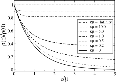
Figure 2: Leading order counterion density in the SC limit for different values of $\kappa\mu$. For the sake of representation, we show the ratio of density to its contact value, $\rho_{c}^{0}(z)/\rho_{c}^{0}(0)$, as obtained from eq. (12).

Let us now consider the validity of the SC-DH theory by comparing the leading order counterion distribution eq. (12) with the next leading contribution eq. (15). This gives a validity condition in terms of $\tilde{z}^{2}<2\Xi/(1-\kappa\mu\Xi)$, that makes sense as long as $\kappa\mu<\Xi^{-1}$. This means in fact that the SC-DH theory is valid for larger distances from the wall when compared to the zero-salt case [17]. This is clearly in accord with the features of the phase diagram in fig. 1, where by adding salt the SC-DH expansion eventually becomes valid for all separations from the wall. In the regime $\Xi^{-1}<\kappa\mu$, this validity condition is always satisfied. In reality, this regime is easily applicable, since this condition can be written as $q_{c}^{2}\kappa\ell_{\mathrm{B}}>1$. In physiological salt conditions with $\ell_{\mathrm{B}}\simeq 0.7{\mathrm{nm}}$ and $\kappa\simeq 1{\mathrm{nm}}^{-1}$, this reads as $0.7q_{c}^{2}>1$, which is already satisfied for divalent counterions.

Finally, in the regime $\kappa\mu>1$ we need to generalize the calculation to take into account corrections of order $(\kappa\mu)^{2}$ to the next leading counterion density $\rho_{c}^{1}(\tilde{z})$ in eq. (15). This calculation will be presented in the forthcoming publication [22].

Furthermore, one has to notice that eq. (15) holds only in the case when the interaction between positive ions and negative salt ions does not give any significant contribution to the densities. These plus-minus attractions induce an extra length-scale to the problem, the radius of ions $a$, which has to be non-zero to cut off these interactions. In the limit $\kappa\mu\rightarrow 0$, i.e. when the interaction between ions is assumed to be unscreened, the results derive above hold as long as

$$\kappa\mu<\frac{2\tilde{a}}{\Xi}+\mathcal{O}(\ln[\kappa\ell_{\mathrm{B}}/(\kappa a)^{2}]),$$ (19)

where $\tilde{a}$ is the rescaled ion-radius [22]. This clearly means, that we cannot reduce $a$ to zero without removing all the salt, i.e. setting also $\kappa\mu=0$. This is clearly caused by the fact, that even in the presence of very small amount of negative salt ions the Mayer functions of oppositely charged ions start to diverge, indicating complexation into Bjerrum pairs.

In summary, the SC-DH limit, where typically one has $\tilde{a}=a/\mu\gg 1$, thus applies to the leading order for all values of $\tilde{z}$ , as long as $\Xi^{-1}<\kappa\mu<2\tilde{a}/\Xi$. The criterion eq. (19) does not necessarily imply that the SCDH limit becomes invalid for larger values of $\kappa\mu$. If $\kappa\mu$ exceeds the value given by eq. (19), one has to take into account the screening of interactions even between positive and negative salt ions themselves, thus making SCDH theory applicable for all values of salt concentrations [22].

The presence of these screened interactions increases the density of positive ions close to a charged wall and decreases the density of negative salt ions [22]. Intuitively, this is the case because single-particle density for positive ions is a decreasing and for negative ions an increasing function of distance from the wall. In the SC-limit, the plus- minus interaction is the dominant contribution to the second order virial expansion term. To maximize attraction between negative and positive ions all the density profiles become more sharply peaked close to the wall. However, this happens in such a way that electroneutrality holds, which furthermore means that the integral over the total charge density has to vanish to all higher orders. As a consequence, close to the wall, the amount of positive ions increases, and the amount of negative ions decreases. Clearly, the opposite happens far away from the wall.

The second important contribution to next-leading order densities arises from the subtraction of artificial DH salt bath. This again gives positive contribution to positive ion density and negative contribution to negative ion density close to the wall, and is due to the fact that one is removing perturbatively the artificial ions involved in the screening, thus decreasing the contact densities of negative ions and increasing the contact density of positive ions.

The asymmetric virial expansion presented above also applies to the high salt limit $\kappa\mu\rightarrow\infty$ as long as $\Xi\gg 1$. In this limit, the Mayer functions become extremely short-ranged due to an almost complete screening of electrostatic interactions. As a consequence, one can expand these functions in $v_{\mathrm{DH}}$, giving rise to an expansion independent of $\Xi$. This expansion is valid only if $v_{\mathrm{DH}}(2a)\ll 1$, where $2a$ is the ionic diameter. To the leading order, however, the density expressions derived above apply also to high salt case [22].

The present theory can be readily employed for further, more complex applications including charged polymers and colloids with biologically relevant concentrations of salt. One can also explore situations involving the joint interplay of counterions and salt within the present theoretical framework, which will be discussed elsewhere [22].

Another phenomenon that we have not yet accounted for thus far is overcharging and/or charge inversion observed in simulations of charged surfaces with multivalent counterions in salt solution [30, 31, 32, 33, 34, 35]. This phenomenon has also been extensively studied in several recent theoretical works [16, 27, 28, 29, 36]. It is understood that ion-ion electrostatic correlations [16, 29] as well as excluded-volume effects due to finite ion size [36, 32] play essential roles in the mechanism of overcharging. Physically, the absence of this effect in our formalism so far may be traced back to the limiting one-particle structure of the leading-order SC-DH theory. A thorough analysis of higher-order terms is required to account for many-body and excluded-volume effects which go beyond the scope of the present paper and will be presented in a forthcoming article [22]. It can be shown that the validity of the SC-DH theory strongly depends on the value of the ion-diameter through Mayer-functions, and can actually break down in the limit where the interaction between oppositely charged particles exceeds $k_{\mathrm{B}}T$, which is already indicated by eq. (19). This limit indicates the onset of Bjerrum-pairing, thus destroying the Debye screening picture [22]. Our preliminary simulations [37] indicate that at large coupling parameters overcharging is indeed possible but typically amounts to a fraction of the bare surface charge, which in this feature agrees with other simulations [31, 32, 33, 34, 35] and appears to reflect the second-order nature of this phenomenon.

In summary, we have derived analytic expressions for counter- and co-ion distributions in the presence of salt in the vicinity of a charged macroion. The results are consistent with previous work in the PB, DH and SC limits and fill the gap between the no-salt and high salt limits. The results presented here are relevant in a multitude of soft-matter and biological systems characterized by non-negligible salt concentrations, and pave the way for further applications [22], complementing those presented here.

Acknowledgement – P. L. H. would like to thank the Danish National Research Foundation for its financial support in the form of a long-term operating grant awarded to MEMPHYS–Center for Biomembrane Physics. This work has, in part, been supported by the Academy of Finland, Finnish Cultural Foundation, and the Danish National Research Foundation.

References

- [1] \NameBoroudjerdi H., Kim Y.-W., Naji A., Netz R. R., Schlagberger X. Serr A. \REVIEWPhys. Rep.4162005129.
- [2] \BookHandbook of Biological Physics \EditorLipowsky R. Sackmann E. \Vol1 \PublElsevier, Amsterdam \Year1995.
- [3] \NameIsraelachvili J. \BookIntermolecular and Surface Forces, 2nd edn. \PublAcademic Press, London \Year1991.
- [4] \NamePodgornik R., Harries D., Strey H. H. Parsegian V. A. \Bookin Gene and Cell Therapy, Second Edition, Ed. Nancy Smyth Templeton \PublM. Dekker, New York \Year2004.
- [5] \Namevan der Shoot P. Bruinsma R. \REVIEWPhys. Rev. E712005061928.
- [6] \NameKjellander R., Marcelja S. Quark J. P. \REVIEWJ. Colloid Int. Sci.1261988194.
- [7] \NameWennerström H., Khan A. Lindman B. \REVIEWAdv. Coll. Int. Sci.341991433.
- [8] \NameKekicheff P. , Marcelja S., Senden T. J., Shubin V. E. \REVIEWJ. Chem. Phys.9919936098.
- [9] \NameAllahyarov E., Gompper G. Lowen H. \REVIEWPhys. Rev. E692004041904.
- [10] \Name Neu J. C. \REVIEWPhys. Rev. Lett.8219991072.
- [11] \NamePodgornik R. Zeks B. \REVIEWJ. Chem. Soc. Faraday Trans. 2841988611.
- [12] \NameNetz R. R. Orland H. \REVIEWEur. Phys. J. E12000203.
- [13] \NamePincus P. A. Safran S. A. \REVIEWEurophys. Lett.421998103.
- [14] \NameBurak Y. Andelman D. \REVIEWJ. Chem. Phys.11420013271.
- [15] \NameRouzina I. Bloomfield V. A. \REVIEWJ. Phys. Chem.10019969977.
- [16] \NameGrosberg A. Yu., Nguyen T. T. Shklovskii B. I. \REVIEWRev. Mod. Phys.742002329.
- [17] \NameNetz R. R. \REVIEWEur. Phys. J. E52001557.
- [18] \NameMoreira A. G. Netz R. R. \REVIEWEur. Phys. J. E8200233.
- [19] \NameNaji A., Jungblut S., Moreira A. G. Netz R. R. \REVIEWPhysica A3522005131.
- [20] \NameDebye P. Hückel E. \REVIEWZ. Phys.241923185.
- [21] \NameMoreira A. G. Netz R. R. \REVIEWEur. Phys. J. D21200183.
- [22] \NamePunkkinen O. et al. \REVIEWto be submitted2007.
- [23] \NameHubbard J. \REVIEWPhys. Rev. Lett.3195977.
- [24] \NameSamuel S. \REVIEWPhys. Rev. D1819781916.
- [25] \NameMayer J. E. \REVIEWJ. Chem. Phys.1819501426.
- [26] \NameFriedman H. L. \BookIonic solution theory, 2nd edn. \PublJohn Wiley & Sons, Interscience, New York \Year1962.
- [27] \NameNguyen T. T., Grosberg A. Yu. Shklovskii B. I. \REVIEWJ. Chem. Phys.11320001110.
- [28] \NameNguyen T. T., Grosberg A. Yu. Shklovskii B. I. \REVIEWPhys. Rev. Lett.8520001568.
- [29] \NameLevin Y. \REVIEWRep. Prog. Phys.6520021577.
- [30] \NameTanaka M. Grosberg A. Yu. \REVIEWJ. Chem. Phys.1152001567.
- [31] \NameMartin-Molina A., Maroto-Centeno J. A., Hidalgo-Alvarez R. Quesada-Perez M. \REVIEWJ. Chem. Phys.1252006144906.
- [32] \NameMessina R., Gonzalez-Tovar E., Lozada-Cassou M. Holm C. \REVIEWEurophys. Lett.602002383.
- [33] \NameLenz O. Holm C. \REVIEWarXiv:0711.0199v12007.
- [34] \NameTrulsson M., Jönsson B., Akesson T. Forsman J. \REVIEWPhys. Rev. Lett.972006068302.
- [35] \NameTrulsson M., Jönsson B., Akesson T., Forsman J. Labbez C. \REVIEWLangmuir23200711562.
- [36] \NameGreberg H. Kjellander R. \REVIEWJ. Chem. Phys.10819982940.
- [37] \NameKim Y. W., Punkkinen O., Naji A., Podgornik R., et al. \REVIEWwork in progress2007.