The optimal phase of the generalised Poincaré dodecahedral space hypothesis implied by the spatial cross-correlation function of the WMAP sky maps
Abstract
Context. Small universe models predicted a cutoff in large-scale power in the cosmic microwave background (CMB). This was detected by the Wilkinson Microwave Anisotropy Probe (WMAP). Several studies have since proposed that the preferred model of the comoving spatial 3-hypersurface of the Universe may be a Poincaré dodecahedral space (PDS) rather than a simply connected, flat space. Both models assume an FLRW metric and are close to flat with about 30% matter density.
Aims. We study two predictions of the PDS model. (i) For the correct astronomical positioning of the fundamental domain, the spatial two-point cross-correlation function of temperature fluctuations in the covering space (where the two points in any pair are on different copies of the surface of last scattering (SLS)) should have a similar order of magnitude to the auto-correlation function on a single copy of the SLS. (ii) Consider a “generalised” PDS model for an arbitrary “twist” phase . The optimal orientation and identified circle radius for a generalised PDS model found by maximising relative to in the WMAP maps should yield one of the two twist angles .
Methods. Comparison of to extends the identified circles method, using a much larger number of data points. We optimise the ratio of these functions at scales Gpc using a Markov chain Monte Carlo (MCMC) method over orientation (, , ), circle size , and twist .
Results. Both predictions were satisfied: (i) An optimal generalised PDS solution was found for two different foreground-reduced versions of the WMAP 3-year all-sky map, both with and without the kp2 galactic contamination mask. This solution yields a strong cross-correlation between points which would be distant and only weakly correlated according to the simply connected hypothesis. The face centres are (and their antipodes) to within ; (ii) This solution has twist , in agreement with the PDS model. The chance of this occurring in the simply connected model, assuming a uniform distribution , is about 6-9%.
Conclusions. The PDS model now satisfies several different observational constraints.
Key Words.:
cosmology: observations – cosmic microwave background – cosmological parameters1 Introduction
The past decade and a half have shown considerable growth in attempts to determine the global shape, i.e. not only the curvature, but also the topology, of the spatial comoving section of the Universe, i.e. of the 3-manifold to which a 3-hypersurface corresponds, informally known as “space”. As noted by several authors, in particular Starobinsky (1993) and Stevens et al. (1993), a space that is “small” compared to the surface of last scattering (SLS) cannot contain eigenmodes, which are used for expressing density perturbations, which are themselves larger than the space itself. This should lead to a cutoff of power in statistics representing these fluctuations, above which power should drop to zero. This prediction was made after COBE data were available, but before the WMAP satellite was launched. For practical, observational reasons, spherical harmonic analyses of temperature fluctuations on the 2-sphere are frequently made. However, a physically more natural statistic to use is one in three-dimensional space, e.g. the two-point auto-correlation function.

The predicted cutoff in large-scale power appears to have been confirmed by the first-year observations of the Wilkinson Microwave Anisotropy Probe (WMAP) experiment. With this data, Spergel et al. (2003) published a figure approximately equivalent to such a function, i.e. the black “WMAP data” curve of Fig. 16 in their paper. Their figure shows the auto-correlation calculated as a function of angular separation, shown against projected spatial separation for a (first year) template-cleaned V map with the kp0 galactic contamination mask. The authors note the surprisingly flat correlation on large scales and suggest a multiply connected universe model to match this function.
In Fig. 1, we calculated the auto-correlation function directly as a function of three-dimensional spatial separation, not of angular separation, using the 3-year integrated linear combination (ILC) map with the kp2 cut. This figure can be approximately compared to the black “WMAP data” curve of Fig. 16 of Spergel et al. (2003), except that the present figure shows the auto-correlation calculated as a function of three-dimensional spatial separation, not of angular separation; the relation between the two is not linear. Also, our figure uses the 3-year ILC map with the kp2 cut, not the 1-year template-cleaned V map with the kp0 cut.
In spatial comoving units, we confirm that the auto-correlation is very close to flat for separations larger than . The relation between angular and spatial scales is, of course, not linear. Equation (17) below (for either a spherical covering space or for a flat covering space using the limit ) can be used to calculate this.
If the size of the Universe111See e.g. Fig 10 of Luminet & Roukema (1999) for a schematic diagram of various definitions of the “size” of the fundamental domain, including the injectivity radius, the in-radius, and the out-radius. is about 10 Gpc, as this figure seems to indicate, then which of the various 3-manifolds correctly describes comoving space? Motivated by indications that the Universe may have positive curvature, and using eigenmode-based simulations to study the spherical harmonic () spectrum of the WMAP data, Luminet et al. (Luminet et al. 2003; Caillerie et al. 2007) argue that the Poincaré dodecahedral space (PDS) is favoured by the WMAP data over an infinite, simply connected flat space. Caillerie et al. (2007) state that, by requiring maximal repression of the quadrupole signal, an optimal total density of is favoured (for a non-relativistic matter density and Hubble constant km s-1/Mpc) for the PDS model. Several other authors (Aurich et al. 2005a, 2005b; Gundermann 2005) have also compared simulations for PDS models to the observed first-year and three-year Wilkinson Microwave Anisotropy Probe (WMAP) maps of the cosmic microwave background (CMB).
In all these studies, both the infinite flat models and the PDS models are used in the context of a standard, hot big bang model, i.e. where the Universe has a Friedmann-Lemaître-Robertson-Walker (FLRW) metric, perturbed by fluctuations that collapse gravitationally to form structures such as filaments and clusters of galaxies, and where values of the metric parameters consistent with the consensus obtained during the last decade of observations are adopted: the Universe is close to flat on length scales up to the SLS and has about 30% non-relativistic matter density.
In other work, Roukema et al. (2004) used the identified circles principle (Cornish et al. 1996, 1998) to find a specific optimal orientation of the PDS model based on the WMAP first-year ILC map, and published a tentative set of coordinates. Key et al. (2007) confirmed the presence of a signal at the celestial coordinates, circle radius, and twist published in Roukema et al. (2004), but argue that it should be considered a false positive. Using software independent of that used in Roukema et al. (2004), updating to the 3-year WMAP data, and using Gaussian simulations, Lew & Roukema (2008) find similar conclusions. They find that a local maximum in the statistic used for finding matched circles exists for a circle radius and a twist, but it is not statistically significant.
Aurich et al. (2006) also made a circles analysis of the WMAP first-year data, using their own estimator and weight function, and, in contrast with Roukema et al. (2004), Key et al. (2007), and Lew & Roukema (2008), did not find any signal at . On the other hand, they did find a tentative PDS signal at , or equivalently, a circle radius . The signal is weaker than they expected, but the authors note that uncertainties due to foregrounds and noise structures in the data make it premature to draw firm conclusions.
A disadvantage of the identified circles approach is that it is based on the information in a relatively small number of points on the sky map of temperature fluctuations, making it sensitive to small errors in the data or analysis and requiring prohibitively long computations. Is it possible to generalise from the identified circles principle?
Moreover, leaving aside the debate about matched circles statistics, observably multiply connected models could reasonably be said to have satisfied only one prediction so far, that of a cutoff in the density fluctuation spectrum on a large scale. Can predictions of the PDS model itself be tested, for example, using the identified circles principle or an extension of it?
In searches for matched circles, the statistic used is usually some variation on what can be considered to be the value of the two-point cross-correlation function of observed temperature fluctuations at pairs of points in the covering space, , where the two points lie on different copies of the SLS, and the separation of the two points in the pair (on the different copies of the SLS) is zero in the covering space.
We can write this function as if it were possible to sample temperature fluctuations as point objects at arbitrary spatial points throughout the covering space, i.e. including arbitrarily low redshifts, as well as points beyond the SLS:
| (1) |
averaging over triples satisfying and (the identity is removed because we only want the cross-correlation). Here, for are arbitrary points on the SLS considered to be located at their comoving spatial positions, for are the 12 holonomy transformations in the binary icosahedral group operating on the covering space that match opposite faces of the fundamental polyhedron of the PDS, is the comoving spatial geodesic distance between two points in the comoving covering space (i.e. an arc-length on the covering space embedded in , e.g. Roukema 2001). The temperature fluctuations on one copy of the SLS, , are extended to the whole covering space via the holonomy transformations, i.e.,
| (2) |
The latter assumption, i.e. Eq. (2), enables rewriting Eq. (1) in a way that becomes observationally realistic,
| (3) |
again subject to the conditions that the average is taken over pairs satisfying and . The auto-correlation function can then be written
| (4) |
averaging over pairs satisfying . In words, is the 3-spatial auto-correlation function for pairs of points on a single copy of the SLS, while is the 3-spatial cross-correlation function for pairs of points where the two members lie on different copies of the SLS in the covering space.
Now rewrite the statistic used in matched circles searches as follows [see e.g. Eq. (9) of Roukema et al. (2004), with the normalisations (denominator and monopole ) ignored for simplicity],
| (5) | |||||
for the case where pairs of points are (hypothetically) multiply-imaged locations located on a pair of matching circles in the covering space. We use here because that is the defining characteristic of matched circles — a pair of matching points is a match because the two points are the same space-time points, i.e. they are separated by when their topological images located on adjacent copies of the SLS in the covering space are considered.
Here, generalise from the zero separation cross-correlation to cross-correlations at larger separations . We can expect that
| (6) |
i.e. that correlations weaken with separation and that, in general, should be approximately equal to the auto-correlation function on scales much smaller than the “size” of the fundamental domain, e.g. the in-diameter (e.g. fig 10, Luminet & Roukema 1999)
| (7) |
since there is no statistical, physical distinction between a pair of points on different copies of the SLS and a pair of points on a single copy of the SLS, apart from effects that are not locally isotropic, such as the Doppler effect.
Since is generally large at small and small at large , obtaining a large correlation requires using a range of length scales that are relatively small, e.g.,
| (8) |
should be a relatively high positive value if the multiply connected model being studied is the correct model.
Another way of saying this is that this test compares the spatial two-point cross-correlation function of mapped (in the sense of the holonomy transformation , which maps one copy of a point in the covering space to one of its images) and unmapped temperature fluctuations in the covering space, where the two points in any pair are on different copies of the SLS, against the auto-correlation function on a single copy of the SLS.
To see yet another way of thinking about this, suppose that the PDS model at a given orientation and implied circle size is correct and that temperature fluctuations occur as point objects, each emitting isotropically. The covering space cross-correlation function, based on pairs of points that are close to one another due to the application of one or more holonomy transformations , but are not close to one another on a single copy of the SLS, should then be statistically equivalent (apart from the Doppler effect and foreground/projection effects) to a sampling from the spatial auto-correlation function , which can be estimated using points that lie on a single copy of the SLS.
This gives us our first prediction to test the PDS hypothesis: Eq. (8) should only be expected to hold if the physically correct PDS (or other) 3-manifold is assumed and is modelled at its correct astronomical orientation. If the PDS model is correct but a wrong orientation is chosen, then the cross-correlation inferred from it on small length scales — in the covering space since it is the cross-correlation — should represent correlations of pairs of points that in reality are not close together, due to the erroneous orientation that causes mappings from one copy of the SLS to another to be incorrect. Since the correlation of distant points is, in general, small, we have for this incorrect PDS model:
| (9) | |||||
i.e.
| (10) |
in contrast to Eq. (8). Similarly, if the PDS model is incorrect, then arbitrary orientations should also yield small cross-correlations on small length scales, as in Eq. (10).
In this paper, the initial aim is to maximise relative to , varying PDS models over the parameter space of different orientations and circle sizes. (In the actual calculations, we used a range of scales below and a little above : see Sect. 3.3 and Eq. (20) for details.) This should lead to an estimate of the best orientation and circle size for the PDS model, given the observational data.
However, to further test the PDS model, consider a “generalisation” from the mathematically correct PDS model to a class of pseudo-models for which the cross-correlation function can be calculated, but for which most222The mathematical term “almost all” could be used here, but when taking observational and numerical calculation uncertainties into account, the word “most” is more realistic. of the members of the class are physically invalid. Maximising (relative to ) over the extended parameter space defined by this class should then have little chance of yielding an optimal model that is valid, unless the PDS model is astronomically correct.
The “generalisation” that we define here is to allow the “twist” angle to be arbitrary in . The twist angle can be described as follows. In a single-action, spherical 3-manifold (e.g., Sect. 4.1, Gausmann et al. 2001) thought of as embedded in 4-dimensional Euclidean space, , any holonomy transformation is a Clifford translation that rotates in about the centre of the hypersphere in one 2-plane by an angle of , and also by in an orthogonal 2-plane.
From a close-up perspective of the SLS rather than looking at the whole hypersphere , or in other words, from a projection into , one 4-rotation can be thought of as a translation in from one circle in a matched circle pair to the other member of the pair on the opposite side of the SLS, and the second 4-rotation is then thought of as a twist around a vector in the translation direction joining the centres of the two identified circles. This full motion is frequently termed a “screw motion”. The “twist” is the second of these two rotation angles.
Physically, the only two possible twist angles are If the cross-correlation were to be calculated by filling one copy of the fundamental domain with a uniform distribution of points and then mapping this set of points to copies of the fundamental domain in the covering space, then for an invalid twist angle, some regions of space near the first copy would have either zero, two, three, or more times the density of points in the first copy of the fundamental domain. In other words, sharp discontinuities would occur in calculating the cross-correlation.
However, a practical way of estimating the cross-correlation is the method represented in Eq. (5), i.e. multiplying temperature fluctuations and then averaging them. Using this method rather than multiplying densities of points, the effect mentioned in the previous paragraph should only lead to slightly more or less frequent sampling in some regions of the cross product of the covering space with itself, not to a modification of the correlations themselves.
The continuous nature of this method, as opposed to the discrete nature of starting with a uniform distribution of points in the fundamental domain, can be seen as follows. For a given pair of observed locations on one copy of the SLS, their comoving spatial separation for a given “generalised” isometry , which depends on the generalised twist , changes continuously through the values not discretely. Moreover, the product of the observed temperature fluctuations remains constant. Intuitively, we could say that as varies, the geodesics formed by pairs do not “know” when they meet other pairs , where and are two holonomy transformations mapping the fundamental domain to two copies of the fundamental domain adjacent to one another in the covering space.
If the PDS model is correct, then calculating using temperature fluctuations and applying isometries using an arbitrary twist angle should give as in Eq. (10), but give as in Eq. (8) when the twist angle is correct.
This gives the second prediction of the PDS model. The maximal cross-correlation for this generalised PDS model estimated using correlations of temperature fluctuations should not only exist as a robust maximum, but it should also give a twist angle of either .
If the simply connected, perfectly flat model is correct, then the PDS model is incorrect, and it should either be difficult to find a robust maximal correlation in this extended 5-parameter space, or else an arbitrary twist angle should result, with only a small chance of being close to either of the two values expected for the PDS.
An estimate of how close an “arbitrary” twist angle should lie to one of the two PDS values can be made as follows. Given the assumption that
| (11) |
we can expect that this arbitrary angle should be selected from a uniform probability density distribution on . In principle, depending on the assumptions made about the complex statistical properties of the WMAP temperature fluctuation maps, it could be possible for this distribution to be non-uniform, even for a non-PDS space model. However, the estimated spatial auto-correlation function for Gpc is close to zero, as shown in fig 16 of Spergel et al. (2003) as a function of angular separation on the SLS (), and explicitly as a function of spatial separation in Fig. 1 here, so the assumption does appear to be supported by the empirical evidence.
For the uniform distribution assumption, let us define
| (12) |
for . The chance of the observational optimal phase being close to or is then
| (15) |
The piecewise nature of this function is because; e.g. there are four ways in which can differ from by a small angle such as , but only two ways in which it can differ from by a large angle such as .
To search for an optimal solution in the parameter space, a Metropolis-Hastings version of a Markov-chain Monte Carlo (MCMC) method is used (e.g., Sect. 4.2, Neal 1993, and references therein) over the five-dimensional parameter space
| (16) |
where the parameters represent dodecahedron orientation (, , ), circle size and twist phase . All parameters are initialised as arbitrary angles, except that the circle size is constrained to both initially and during the whole chain. See Sect. 3.6 for more details.
We also ran some MCMC chains starting with the parameters of the Roukema et al. (2004) “hint” of a PDS solution with circles of size . If this solution is correct, then we would expect the chains to remain localised around that same solution. If the solution is wrong and if a correct solution exists, then the chains should move towards that correct solution, even though starting at a wrong point. If the solution is wrong and if no correct solution exists, then we would expect the chains to move randomly and fail to find a strong maximum.
The correlation function definitions are described in Sect. 3.2, the probability estimator used to compare multiple-SLS cross-correlation and single-SLS auto-correlation functions is presented in Sect. 3.5, and the MCMC method is described in Sect. 3.6. Results are presented in Sect. 4. Discussion follows in Sect. 5 and conclusions are made in Sect. 6.
For references on cosmic topology in general, please see the first known article on the subject (Schwarzschild 1900, 1998), a short beginner’s review of cosmic topology (Roukema 2000), more in-depth reviews (Lachièze-Rey & Luminet 1995; Luminet 1998; Starkman 1998; Luminet & Roukema 1999), workshop proceedings (Starkman 1998; Blanlœil & Roukema 2000), and lists of two-dimensional and three-dimensional methods (Table 2, Luminet & Roukema 1999; Uzan et al. 1999; Roukema 2002; Rebouças & Gomero 2004). For background on spherical, multiply connected spaces, see Weeks (2001), Gausmann et al. (2001), Lehoucq et al. (2002), Riazuelo et al. (2004), and Luminet et al. (2003). For the identified circles principle, of which the present method can be thought of as an extension, see Cornish et al. (1996, 1998).
One correction to a point made in much of the above literature concerns the independence of the metric and global topology. For example, Luminet & Roukema (1999) wrote, “However, general relativity deals only with local geometrical properties of the universe, such as its curvature, not with its global characteristics, namely its topology”. The error here is that global topology can, at least in certain cases, generate a local effect, and thus affect local geometrical properties. See the , Newtonian weak field limit, heuristic calculation in Roukema et al. (2007): if the Universe contains inhomogeneities and is not expanding perfectly isotropically, then at least in the case, additional accelerations and decelerations exist in the different fundamental directions, in such a way that they tend to equalise the slightly different expansion rates.
Comoving coordinates are used when discussing distances (i.e. “proper distances”, Weinberg 1972, equivalent to “conformal time” if ). We write the Hubble constant as km s-1/Mpc.
2 Observations
The analysis presented here uses the Internal Linear Combination (ILC)333http://lambda.gsfc.nasa.gov/data/map/ dr2/dfp/wmap_ilc_3yr_v2.fits all-sky map of the three-year WMAP data (Spergel et al. 2007) and the Tegmark et al. (2003) foreground-cleaned, Wiener-filtered (TOH)444http://space.mit.edu/home/tegmark/ wmap/wiener3yr_map.fits version of the same data. (Unless otherwise stated, we refer to the three-year data, not the one-year data.)
For our main analyses, we used either the “kp2” mask to eliminate the Galactic Plane (GP) and associated regions from the analysis555Data file: http://lambda.gsfc.nasa.gov/data/map/ dr2/ancillary/wmap_kp2_r9_mask_3yr_v2.fits, map projection: http://lambda.gsfc.nasa.gov/product/map/ current/map_images/f02_int_mask_b.png. or no mask at all. We also discuss analyses with the “kp0” mask. The kp2 mask covers about 15% of the sky, and the kp0 mask covers about 25% of the sky.
We did not carry out any explicit smoothing of these maps, though the MCMC method itself could be thought of as a method that (when analysed statistically) implicitly smooths the information in the data.


3 Method
A GPL (GNU General Public Licence) program circles666Version circles-0.2.4 is the one used for the main calculations in this paper, along with circles-0.2.4.f13.3, which differs from the former only in the formatted printing of galactic longitude to standard output and to a file. Various versions of the packet are downloadable from http://adjani.astro.umk.pl/GPLdownload/dodec/. The software presently requires medium to advanced GNU/Linux, Fortran77 and C experience for a scientific user. is available for reproducing the analysis as described below. A typical 12,000 step MCMC chain as described below should take about 3–4 days to run on an x86 type processor running at about 1.5-2 GHz.
3.1 Spatial versus angular correlation functions
Since the naïve Sachs-Wolfe effect is due to locally isotropic emission, which is what makes the identified circles test useful for the purposes of testing cosmic topology hypotheses, we will assume the same approximation as that required for the circles test to reveal a signal, i.e. that the integrated Sachs-Wolfe effect and the Doppler contribution are relatively small on the observational angular scales corresponding to the length scales of interest. At worst, this assumption should weaken any signal found; it is difficult to see how it could create a false signal. This assumption is written below in Eq. (2).
3.2 Auto- and cross-correlation functions: vs
Due to observational constraints, the spatial auto-correlation function that we are interested in for this test is usually estimated indirectly, e.g. in angle, and calculated in terms of spherical harmonic components of the temperature fluctuations considered as a function on the sphere.
However, the angular correlation function on the SLS is sometimes calculated. Figure 16 of Spergel et al. (2003) shows the main feature useful for this test: to first order, the correlation is high at low separations and low at high separations. As mentioned above, the figure also shows both the disagreement between the simply connected flat model and the observations and the surprising flatness of the correlation function over most angular scales greater than about 40–50∘.
Figures 2 and 3 show what is described algebraically in Eqs. (10) and (8): in a simply connected model, , while in a multiply connected model at the correct orientation and identified circle size, . For simplicity, these two diagrams show only one holonomy transformation . A holonomy transformation is an isometry of the covering space used to define the PDS, i.e. where , the binary icosahedral group, is the group of isometries dividing the covering space into 120 multiple copies of the fundamental domain.
The auto-correlation, , is calculated using Eq. (4). To calculate for a given orientation and circle size, we used Eq. (3), with all 12 of the holonomy transformations (those giving the first “layer” of spherical dodecahedra neighbouring the “first” copy of the fundamental domain).
In principle, Eq. (3) could be evaluated over a “large” subset of all members of the subgroup generated by the holonomy transformations, e.g. . However, this would be highly redundant. The minimum number of calculations that should be done to test a reasonably large sample of different pairs would be those within one copy of the fundamental domain, plus pairs crossing the boundaries of that copy of the fundamental domain.
This leads to an alternative way of visualising . It could be thought of as the auto-correlation function of the full set of all temperature “fluctuations” (or pixels for a given pixelisation of the sphere) mapped into one copy of the fundamental domain, plus those crossing “boundaries”.
In practice, we find it simpler to work in the covering space and to use just the set of holonomy transformations that give the neighbours of a single copy of the fundamental domain, rather than the full group of 120 holonomy transformations.
3.3 Comoving lengths and angular scales

Physically, the separations of interest are lengths of spatial geodesics in the covering space — the hypersphere. This is used for both the simply connected and PDS assumptions, since there is no problem having just a single SLS embedded in an covering space. These separations can be thought of as arclengths or the angles that subtend them on that hypersphere, of radius (e.g. see eq. (2) of Roukema et al. 2004), embedded in Euclidean 4-space (e.g. Roukema 2001), but these angles are different from angles on the SLS (a 2-sphere of radius ) as seen from an observer at the centre of that 2-sphere.
Fig. 4 shows some key relations within the SLS. From the left-hand triangle, use of the spherical sine and cosine formulae leads to
| (17) |
for the ratio of the SLS () radius, , to the radius of the full hypersphere (), , where is the radius of a matched circle () on the SLS. For the right-hand triangle a single application of the spherical sine formula is sufficient to obtain an expression for relating the geodesic (3-sphere) distance between a pair of points to an angle more familiar to observers of the cosmic microwave background:
| (18) |
However, what is of interest in the present work is to estimate the spatial correlation functions in comoving space rather than angular correlation functions on the SLS. While it is possible to define a meaningful relation between and when both and lie on the SLS, a more general distance betweeen and for one of the 12 holonomy transformations cannot easily be interpreted as an angle , since, in general, does not lie on the SLS.
For the auto-correlation function, there is only one copy of the SLS, so the maximum separation at which could, in principle, be calculated is the diameter of the SLS, i.e. .
For the cross-correlation, since copies of the SLS fill (redundantly, with overlaps) the covering space (the hypersphere), the maximum separation that could, in principle, be used for estimating is .777If the covering space were infinite, then there would be no upper limit to the distances at which the cross-correlation could be calculated, independently of whether or not at these separations were meaningful. This is several times larger than . However, correlations across more than half the size (e.g. injectivity radius) of the fundamental domain contain information redundant with those at smaller separations.
Moreover, as mentioned above, we focus on a range of length scales that are small enough that the auto-correlation is (certainly) high and the cross-correlation (in the case of a correctly oriented PDS, if it is physically correct) is also high. Above we suggested Gpc. Figure 1 shows the auto-correlation function estimated from the ILC WMAP map using the kp2 galactic contamination mask. The correlations are high for Gpc and remain positive for Gpc. They are approximately zero for separations greater than one SLS radius:
Since we want to use a range of small scales, not just a single scale, the specific range used in calculations here was
| (19) |
i.e.
| (20) |
for , . The fraction is by analogy with degrees, but as shown in Fig. 4 and Eq. (18), this does not relate linearly to an angle on the SLS and is better considered as an arbitrary unit. The approximate correspondence in angles on the SLS, as given in Eq. (18), is approximately .
Since a relatively small number of points, , is used in estimating the correlation, and since we bin into separation intervals, the inclusion of pairs with smaller separations, Gpc, would be likely to provide only a small, noisy contribution to the total correlation. Using these closer pairs without introducing too much noise would require increasing , thereby slowing down the calculations. Nevertheless, this could be examined in future work. See Sect. 3.5 for the values of and adopted number of bins.
3.4 Calculating the holonomy transformation from a pair of matched circles
In Roukema et al. (2004), circle pairs were examined without calculating holonomy transformations of the 3-manifold, since that was not needed.
Although it is possible to explore the parameter space of different possible 3-manifold sizes and orientations directly from sets of holonomy transformations without any initial reference to identified circles, since the latter are derived from the former, we find it easier to start from the latter.
We represent the parameter space of these different possibilities by the coordinates of the face centres of a fundamental domain (spherical dodecahedron), as stated above. In this case, it is possible to reconstruct the holonomy transformation for a circle pair for the PDS corresponding to that circle pair, given the positions of the two matching circles. Consider the centres of the two corresponding circles as euclidean vectors in , where is a four-dimensional matrix representation of the holonomy transformation as a left multiplier whose values numerical values are not yet known. Using the term “eigenplane” as introduced in Roukema (2005), these two vectors determine one of the two eigenplanes of the isometry , as described in Eq. (15) of Gausmann et al. (2001).
As in Section 2.3.3 of Roukema (2005), using and in Eq. (19) of Roukema (2005) gives a second vector, , in this same eigenplane, orthonormal to :
| (21) |
where is the inner product on .
Since lies in the same eigenplane and resolves to the same components in the plane as , apart from a rotation by , it follows that
| (22) |
We find a third vector starting with one of the four Cartesian axis unit vectors (that which is furthest in angle from )
| (23) |
A fourth vector is defined as the cross product of , , and , which can be calculated by writing these three vectors as row vectors , , and , respectively and estimating the determinant of the appropriate matrix using the four othonormal basis vectors in a given orthonormal basis:
| (28) |
Since the zero point of rotation within the plane is arbitrary, we then define the vectors and :
| (29) |
where is the generalised twist phase mentioned in Sect. 1. We then calculate from
| (30) |
3.5 “Probability” estimator
Our primary aim is to see if we can reject the simply connected model by looking for the signal expected from a PDS model. This does not require a true probability for use in an MCMC search of parameter space. Instead, it is sufficient to have a function similar enough to a probability function that the chains will explore the full parameter space and converge after a reasonably short amount of computing time and that they will show where the maximal correlation lies.
For a given set of parameters [see Eq. (16)] defining a sixtuplet of circle pairs, points are selected from a uniform distribution on the 2-sphere. The auto- and cross-correlations and are calculated for all and pairs, respectively, applying Eqs (3) and (4), respectively. Many of these pairs, especially in the latter case, fall at separations too large to be of interest for our test. We bin the pairs into bins in the comoving separation range given by Eq. (20).
We define the “probability” that the function at a given point in parameter space is sampled from the known, “true” correlation, i.e. the auto-correlation , by assuming a Gaussian distribution of errors of width in each -th bin (unless ) and assuming that the bins are independent:
| (36) |
Values are replaced by so that the MCMC chains are ergodic (e.g., Sect. 4.2, Neal 1993).
The definition of the distribution width, , is based on numerical experimentation in order to obtain an optimal fit with the MCMC method in a reasonable amount of time:
| (37) |
where is the number of pairs contributing to the -th bin in the estimate of . For the largest bin, , which gives width , so a cross-correlation in this bin needs to be as high as to contribute a probability per bin of or higher to the full product. The weighting increases in bins where there are fewer pairs (normally those with ), thereby moderately decreasing the strength of those bins’ contributions to the product in Eq. (36), so that bins with relatively high Poisson errors do not penalise the probability too much. In practice, the maximum of reaches , for and bins in the range given in Eq. (20).
For bins in which , use of the upper expression in Eq. (36) would lead to penalising these bins for giving unexpectedly strong cross-correlations. Would this be reasonable? When cross-correlating points that are physically close in comoving space but observed at widely separated angles, it is conceivable that the avoidance of foreground effects could lead to in some bins, in which case we would want to favour these contributions. To know whether any significant effect should be expected in practice would require full modelling of the Doppler and integrated Sachs-Wolfe effects.
However, while it is unclear how significant any such effect would be, it seems clear that we should not penalise the bins in which . Here, a very slight excess probability per bin is applied in these bins, as defined in the lower expression in Eq. (36). A bin in which the cross-correlation is as high as , which is much higher than is likely to occur in practice, would yield a probability per bin of to the full product, so the contribution in practice is likely to be small; i.e., there should be a slight preference for excess cross-correlations with respect to auto-correlations.
3.6 Markov Chain Monte Carlo method: Metropolis-Hastings algorithm
The function defined in Eq. (36) is used to explore the parameter space defined in Eq. (16), maximising using an MCMC method with a Metropolis-Hastings algorithm.
An informal description of this method follows. Starting from a randomly selected point in parameter space, a “chain” of successive points in parameter space is calculated, such that a new step in the chain is taken with certainty when the new probability at a newly chosen test step is higher than the present step, but may or may not be taken if the probability at the new step is lower. The probability of advancing in the latter case is the ratio of the new probability to the probability at the present step. This enables a chain of steps to seek the region of highest probability, while not getting stuck in noisy areas or local hills. For a more formal and complete description of the method, see, e.g. Neal (1993), and references therein, and in particular, Section 4.2 of that paper.
At each step, the -th parameter is chosen randomly using a uniform distribution on . The proposal distribution in the Neal (1993) notation is a Gaussian distribution on this -th parameter, centred on the previous state , of width
| (38) |
where ∘ indicates great circle degrees. The Gaussian is truncated (without renormalisation) in at and .
The probability as defined in Eq. (36) is used in Eq. (4.18) in Neal (1993) for the acceptance function . The initial state (point in parameter space) is selected randomly from uniform distributions in
The region of space used for choosing the initial values is highly redundant. The range in defined here covers a fraction of the surface of the sphere; while in principle it only needs to cover of the sphere, i.e., there is a factor of redundancy.
The range in the initial choice of “rotation” angle is due to the nature of the dodecahedron. A single choice of defines a class of dodecahedrons that share one pair of faces joined by the axis joining to its antipode . Rotation about this axis by gives a class of distinct dodecahedra, but rotation by for any integer gives the same set of face centres.

In the chains, the numerical values of are all allowed to increase or decrease arbitrarily, beyond the ranges chosen initially. This is for calculational simplicity, both for speed and for minimising the chance of introducing errors into the software. Together, the triple is likely to cover only a relatively small fraction of that part of the non-periodic Cartesian product space of the three parameters defined by the least and greatest numerical values of and reached in a given chain.
During analysis, probably the simplest way to reduce the redundancy is by converting each triple to a 12-tuplet , where the first face centre is numerically equivalent to , converted to a conventional numerical range (e.g. ). Although the set of face centres should, in principle, consist of 6 antipodal pairs rather than 12 independent sky positions, the freedom given to and the stochastic nature of the MCMC chains and the sampling used to estimate correlation functions imply that the two elements of any antipodal pair will not in practice be perfectly antipodal.
The longest dimension in this parameter space is that of the phase , so this is the dimension that constrains the “burn-in” time. The burn-in time is the number of steps in the chain needed to find the region of maximal probability, i.e. of the strongest cross-correlations relative to auto-correlations, independently of where the chain started from. Since the longest possible “distance” from the optimal region (if that exists) is , the number of steps to cross this by a random walk can be estimated as
| (39) |
steps, where the factor of 5 is due to changing only one parameter at any step.
Thus, for our primary estimate of the optimal point in parameter space, we use chains starting with different random seeds, each run for 12,000 steps. We ignore the first 2000 steps and use the last 10,000 steps for further analysis.
4 Results
For the main calculation, MCMC chains were run, starting with different random seeds for both maps (ILC and TOH), with either no mask or the kp2 mask. Each run had 12,000 steps, except that for the ILC map and the kp2 mask, the total number of chains was greater (). As expected (Sect. 3), each chain took about 3–4 days to run on a GHz x86 type processor on a system running a variety of the GNU/Linux operating system.
The MCMC chains used in this paper can be downloaded for independent analysis from the file http://adjani.astro.umk.pl /GPLdownload/MCMC/mcmc_RBSG08.tbz.
4.1 Optimal dodecahedron orientation: space
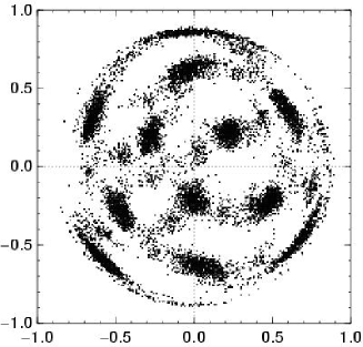
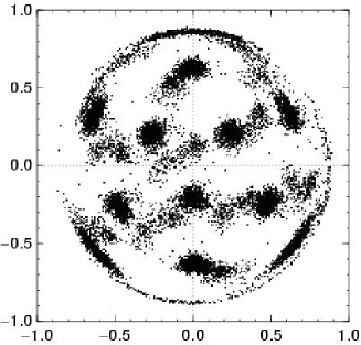
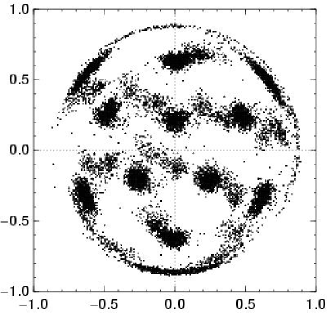
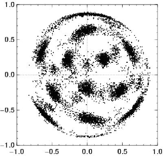
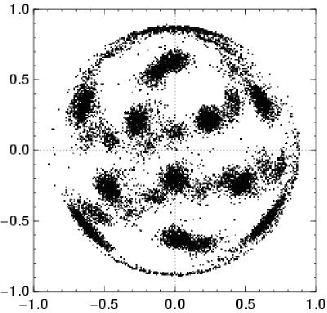
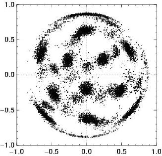
Figures 5, 6, and 7 show the sky positions implied by the triples in the MCMC chains for which (see Eq. (36)). For consistency between the plots, only 10 of the 24 available chains are used to create the plot for the ILC, kp2 case, even though for calculations, we used all 24. The information in the SGP projections (Fig. 6) is equivalent to that in the NGP projections (Fig. 5), so we do not show further SGP projections.
It is clear that a consistent, preferred dodecahedron orientation exists for both the ILC and TOH maps, both with and without masking for contamination by residual foregrounds with the kp2 galactic contamination mask.
We have estimated the preferred values of for the ILC map using the kp2 mask, for which we have 24 chains. Since any individual MCMC chain may fail to find the global maximum due to starting at a distant point in parameter space and random walking in the wrong directions, if we search for preferred values of separately in each chain and then average them and find the dispersion in the estimates, we risk having a large dispersion due to individual chains. On the other hand, if we search for preferred values of in a concatenation of all 24 chains together, we will not have a straightforward way of estimating the uncertainty in the estimates of . Hence, we compromise by grouping the 24 chains together into four groups of six chains888The ordering is random, defined by the numerical values of the random seeds used for the different chains..

For a given group, steps 2001 to 12,000 from each of the six chains are concatenated. An approximate (to within –) estimate of the optimal values evident in Figs 5–7 is
| (40) | |||||
and their six antipodes.999For example, these values can be read off a Mercator projection of the same data. This initial approximation is iterated to yield a more precise estimate. Each iteration uses the mean values of points lying within an angle of the ()-th estimate, starting from , where represents the intial approximation. The angular radii start at (so that most of the sphere is covered), decrease by for the next 10 iterations, and then remain constant at , covering roughly half of the sphere, until the iteration for a given face number converges. For a given threshold , only points for which are used. The means are calculated as means of Cartesian vectors formed from the individual sky positions .
-
a
Apart from restricting to the ranges and respectively, the method is the same as for Table 8.

These four groups of six chains are then treated as four independent estimates in order to estimate the uncertainties due to our MCMC estimation method. These uncertainties are standard errors in the mean calculated in Cartesian space, converted to a one-dimensional uncertainty in great-circle degrees assuming (conservatively) that most of the uncertainty approximately lies in a single dimension:
| (41) |
over groups of chains.
The resulting numerical estimates are listed in Table 1. This table lists sky positions of the best estimates of the six dodecahedral face centres for the ILC map with the kp2 mask, as shown in Fig. 5. The columns show minimum probability , face number , number of MCMC steps contributing to the estimate obtained from the final iteration, galactic longitude and latitude , and the standard error in the mean between these four estimates in great circle degrees, [see Eq. (41)]. The other 6 faces are directly opposite with identical errors. As in Fig. 5, these face centres were derived from the MCMC chains without any constraint on the twist phase .
The final iterated solutions listed in this table are very insensitive to the initial approximation: varying the latter by up to leads to identical final iterations. The table shows that differing thresholds give slightly different solutions, especially in the coordinates of the 5-th face, but these are consistent with each other within the estimated uncertainties.
4.2 Circle size
The optimal dodecahedral face solution shown in Figs 5–7 and Table 1 is inferred from the data without regard to whether the MCMC chains have converged to a preferred circle size and/or twist phase .
We estimated the latter using the same points in the MCMC chains used for the estimate in Table 1. For the circle size , since is restricted to the range we take the mean and standard error in the mean of as a scalar value.
However, there are some reasons to be prudent about the estimate of obtained here. Firstly, relatively large changes in for a fixed dodecahedral face set and a fixed twist can lead to relatively small changes in the distances between a given pair of “close” points on two distinct copies of the SLS, especially when is “small”. This is related to the reason why we expect the cross-correlation method presented in this paper to work: there should be not only many “perfectly matched” pairs of points, in the sense that they are separated by a comoving distance of zero on a single copy of the fundamental domain, but there should also be many other close pairs, extending the matched circle to a “matched annulus”, or in the case of a small circle, a “matched disc”.
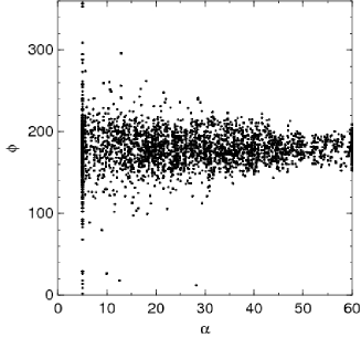
Figure 9 illustrates this. For a fixed twist , each pair of points on the two parts of the sky inside of two matched circles of radius has a separation of at most the separation between the two centres of the circles P and P’, as projected onto the copies of the SLS (not the circle centres in ). From Fig. 9 and Eq. (17) we have
| (42) | |||||
For , a circle radius as large as gives Gpc. Hence, given that we correlate pairs with Gpc, the main cluster of points in Fig. 8 could be interpreted as a “true” matched circle size of 30–40∘.
Secondly, since the width of the step size in the MCMC, [Eq. (38)], is a large fraction of the range in , it is possible that the chains did not have enough freedom to favour a value close to either of these limits, so the statistical nature of the precision of any estimate in is less well-established than for the other parameters, where the chains are totally unrestricted.
Inspection of Fig. 8 suggests that the upper limit, , did not constrain the chains. However, there is a sharp cluster of points at . This is partly an artefact due to not renormalising the Gaussian used in deciding whether to move to the new step in an MCMC chain at the lower cutoff of , as mentioned in Sect. 3.6. Lack of renormalisation artificially increases the probability (by up to a factor of two) of staying near this boundary. This clustering may also be caused by the increased noise at small circle radii. In any case, if the true value of were close to the limit, then the distribution of values around this true value as estimated by this MCMC method could not be a two-sided Gaussian distribution, and even a one-sided Gaussian distribution would not necessarily occur.
Both of these caveats should be kept in mind when using the value from Table 2: the systematic error in this estimate is likely to be much larger than the random error. In this table, as in Table 1, the standard errors in the mean are obtained by treating the four groups of six MCMC chains as independent tests. Listed are minimum probability , number of MCMC steps contributing to the estimate, and its standard error in the mean , and its standard error in the mean , all four in degrees. The number can be a non-integer since for a given MCMC step, it is possible that some of the face centres fall within the convergence radius of the final iteration as described in Sect. 4.1, but other face centres do not.
4.3 Twist phase
As for , we estimated using the points in the MCMC chains used for the optimal dodecahedral face solution presented in Table 1. Since is free to decrease or increase arbitrarily in the MCMC chains, we convert values for these individual points to Cartesian coordinates before averaging and reconvert after averaging. The standard error in the mean is conservative, assuming that all the error occurs in one dimension.
Table 2 shows the estimate of for slightly differing thresholds . Clearly, the value is close to within about one standard error in the mean, with only a slight dependence on the choice of . Figure 8 shows the distribution of and values corresponding to the favoured face centre orientation.
Only one point is displayed for any given state, independently of how long a chain spent at that point, so the visual density of points does not fully match the statistical distribution. Hence, the mean values listed in Table 2 can be offset from the visual centroids in the figure.
What is clear in the figure is that, in addition to the twist phase , a weak secondary feature and a very weak tertiary feature are present, of which the first of these is consistent with the interesting angle of , to within the estimated uncertainty.
We estimate the parameters of these two weak features by using a subset of solution points arbitrarily cut at for the secondary feature and for the tertiary feature. The results are listed in Table 3. Comparison of the numbers of steps in the MCMC chains contributing to the different signals, as listed in Tables 2 and 3, shows that the secondary and tertiary signals are represented by about 10 and 30 times less steps (respectively) than the primary signal.
Clearly, the secondary feature is within 1–2 (standard error in the mean) of , with approximately the same estimated mean circle radius as the primary signal. Only one of the two twist radii can be valid for the spatial matching of opposite faces of the fundamental domain of a PDS model, and they cannot both be valid simultaneously. On the other hand, the density fluctuations in a PDS model must resolve into the eigenmodes of the PDS, not of infinite flat space. It is conceivable that some sort of harmonics could occur, so that secondary and tertiary weak features exist in addition to the main cross-correlation.
4.4 Testing the Roukema et al. (2004) hypothesis
If the PDS solution found here is correct, then the solution suggested in Roukema et al. (2004) cannot be correct (independently of any other arguments), since the parameters are very different.
To test this explicitly, we ran 10 MCMC chains on the ILC map with the kp2 mask, starting at the Roukema et al. (2004) solution. If the latter solution were correct (and if this method is correct), then these chains should remain around that solution. In fact, as Key et al. (2007) appear to agree, the Roukema et al. (2004) solution is at least a local maximum for correlations along matched circles (though they argue that it is not statistically significant, as do Lew & Roukema (2008) using a different method), so the MCMC chains could conceivably remain “stuck” at this local maximum even if a global maximum exists elsewhere in the parameter space. However, Fig. 10 shows clearly that the MCMC chains failed to remain near the Roukema et al. (2004) solution and moved instead to the one found in this paper.
4.5 Probability in the case of a simply connected model
What is the chance that a twist close to could have occurred in a simply connected model? Conservatively taking the 2 upper limits of the estimates of the twist phase of the global maximum found by the MCMCs listed in Table 2, i.e. 5.6-7.8∘, and using the probability distribution for a simply connected model represented by Eqs (12) and (15), the chance of finding to be this close to one of the two PDS values in the case of a simply connected model is about 6-9%.
4.6 Cross-correlation of the preferred solution
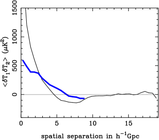
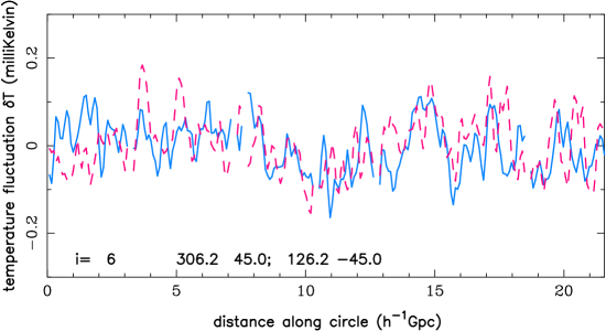
Figure 11 shows the spatial cross-correlation function estimated by assuming that the solution found here is correct (thick curve), together with the auto-correlation function calculated assuming that space is simply connected. The plot is for our solution corrected to an exact dodecahedral solution as indicated in the figure caption.
It is clear that is well above zero in the range and is of about the same order of magnitude as the auto-correlation ; in fact, it is above zero in the range . This is clearly consistent with the PDS hypothesis. On the other hand, according to the simply connected hypothesis, these strong cross-correlations are correlations of temperature fluctuations at points located at positions on the sky separated by well above 10 Gpc. Given the nearly flat, zero auto-correlation measured on scales above 10 Gpc, these temperature fluctuations should be very weakly correlated according to the simply connected hypothesis.
What is striking in Fig. 11 is that finishes — at half the distance separating matching faces of the fundamental domain — just where seems to become flat and zero-valued. This is qualitatively consistent with a PDS interpretation of the “lack of power on large scales”.
4.7 Implied matched circles
The method used in this paper uses random pairs of points of which each point is selected randomly (uniformly) on the 2-sphere, focussing especially on pairs of points that are relatively close.
However, since we used a weighting to focus on bins in pair separations in a way that favours bins with more pairs (Sect. 3.5), and since we used Gpc, corresponding to [Eq. (20)], most of the correlations used to detect the optimal solution are from pairs with Gpc, i.e. , well above our short separation cutoff and well above the map resolution.
While our match is optimal on the scale of several Gpc, it does not necessarily imply a good set of matched circles using individual temperature fluctuations. Moreover, the caveats on the circle size, explained in Sect. 4.2, suggest that, if the PDS solution found here is correct, then its “perfect” matched circle size may well be rather different from the best estimate found here. On the other hand, the first of these caveats suggests that circles should still be approximately matched for wrong estimates of , as long as the true is “small” (e.g. ) and/or the wrong estimate is not too far from the correct estimate.
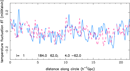
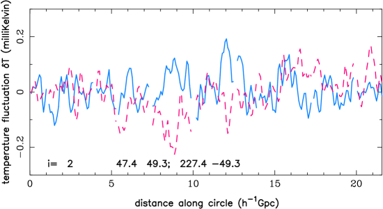
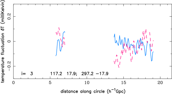
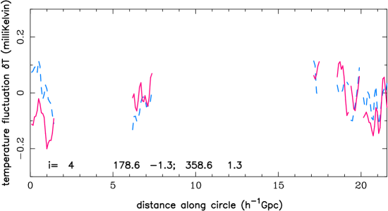
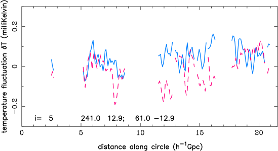
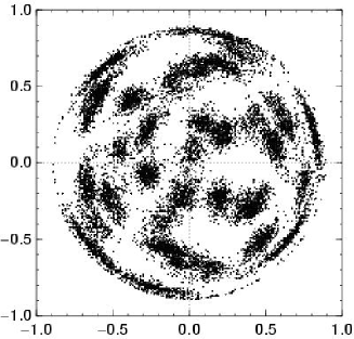
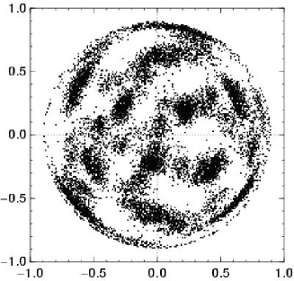
In Figs 12–17, we show the matched circles for the six circles for the corrected solution used in Fig. 11. The two circles in pair 1 clearly have similar overall shapes to one another, as do the two circles in pair 6. Circle pair 2 has some regions that match and some of which do not match. Circle pairs 3, 4, and 5 are badly affected by the kp2 cut, but several of the uncut regions do seem to show some correspondence.
The severe cuts due to the kp2 mask in circle pairs 3, 4, and 5 illustrate a difference between a search for “pure” identified circles and the cross-correlation method, as presented in this paper. Since the cross-correlation method is not limited to zero separation pairs (in fact, it uses very few pairs close to zero separation), it has the advantage of being able to cross-correlate “moderately” close pairs and obtain some signal for the holonomy transformation corresponding to a severely cut circle pair, despite the severity of the cut.
5 Discussion
The PDS model has now satisfied several predictions: not only is there a large-scale cutoff in power, but now we find that (i) a PDS solution maximising the cross-correlation on implied small scales relative to the auto-correlation on certainly small scales exists, and the implied small-scale cross-correlation is of a similar order of magnitude to the auto-correlation on certainly small scales, and (ii) the favoured twist of the “generalised” PDS model agrees surprisingly well with one of the two possible twists to within the accuracy of the method used. Does this mean that the simply connected model should be rejected in favour of the PDS?
Focussing on the second of these tests — the 6-9% chance in the case of a simply connected model of having a twist as close to as what we find here — there are numerous astrophysical, mathematical, and software caveats to be considered. Among these are:
-
(i)
Could this be an effect of galactic contamination that happens to mimic a dodecahedral symmetry with a preferred twist when matching dodecahedral faces?
-
(ii)
Could modifications to the infinite flat model such as our location in a local void (e.g. Inoue & Silk 2006) be sufficient to modify Eq. (15) so that is more likely?
-
(iii)
Could the nature of the comparison test between the auto-correlation and cross-correlation functions itself favour a twist? Could the MCMC algorithm itself be at fault?
-
(iv)
Does a simply connected, infinite flat model really imply a uniform distribution for twist phases ?
-
(v)
The angle as a rotation angle in from one copy of an SLS to another copy of the SLS is necessarily built into the software. Although this rotation is orthogonal to the twist, could it be possible that, due to a subtle programming error, this angle is also built in as a favoured twist angle?
Alternatively, numerous other checks can be made to test the PDS interpretation of this result, including:
-
(vi)
Can this solution be confirmed on smaller scales?
-
(vii)
Are the “secondary” and “tertiary” solutions listed in Tables 3 consistent with PDS harmonics (eigenmodes)?
-
(viii)
Is this solution compatible with other PDS analyses of the WMAP data?
5.1 Galactic contamination?
Could the dominant signal be an effect of galactic contamination? Figures 5–7 show that whether the kp2 mask, covering about 15% of the sky, or no mask at all is used, the same solution is clearly dominant, both for the ILC map and the TOH map. If galactic contamination were significant, it should show up more strongly in the plots with no masking. Indeed, Figs 5–7 show that some weak amount of extra signal, offset from the main solution, does seem to appear when no mask is used, consistent with an interpretation as galactic contamination. The main solution remains dominant.
These figures only show the orientation of the dominant solution. Could the twist itself be due to the shape of the mask, e.g. due to correlating “western” mask edges with “eastern” mask edges? This seems unlikely, but Table 4 confirms that the twist is present with very similar values when no mask at all is used. Each case in this table is for 10 chains. These are divided into two groups, each of five chains. The estimates for a given map/mask combination are thus based on only “independent experiments”, each of five chains concatenated, rather than groups of six chains, so they should be less precise than those for the ILC kp2 case, listed in Table 2.
The estimates in this table are for smaller numbers of chains and so less precise than those for the ILC map with the kp2 mask, but they are clearly consistent with the latter. The signal is therefore unlikely to be an artefact due to the shape of the mask.
Curiously, the best estimates of , together with their uncertainties in Table 4 for the TOH map with and without the kp2 mask, seem to indicate that the further the mean is from , the larger the uncertainty . We have not attempted to interpret this statistically, though it does hint that an alternative way of finding best estimates could lead to a best estimate of closer to , with a smaller uncertainty. As stated at the beginning of Sect. 4, our MCMC chains have been made publicly available for independent analysis.
Returning to the question of possible galactic contamination, could it be possible to be even more conservative and mask more of the sky while not losing the signal? The two-point correlation function depends on the numbers of pairs of points available for sampling a domain. Reducing the coverage of sky by a fraction implies a reduction in the number of pairs by .
This can also be thought of in terms of matched or nearly matched circles. For most choices of the twist , the masked points in one member of a circle pair will correspond to unmasked points in the other pair. Obviously, such pairs cannot be used, even though one of the points lies outside of the masked region. Hence, the masking of pairs grows faster than the masking of individual pixels. The severe cuts in about half of the circles shown in Figs 12–17 illustrate this.
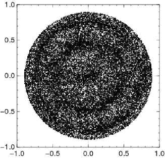
Any further reduction in the amount of sky used risks increasing the presence of noise. A stronger mask used for some studies is the kp0 mask. This covers about 25% of the sky; i.e., about 46% of pairs of points used for estimating correlations are masked. Figures 18 and 19 show the estimates implied by the optimal values in the ILC and TOH maps, respectively, for the kp0 mask. Both figures contain the solution found with no mask or the kp2 mask, but an additional set of optimal points is present, weakly for the TOH map and strongly for the ILC map.
Which of these is more correct? Tegmark et al. (2003) used a method expected to contain less non-cosmological signal from foregrounds and detector noise outside the GP than the ILC method. This would imply that the additional signal that is strong in Fig. 18 and weak in Fig. 19 is more likely to be noise than signal.
In their own study of the first-year ILC and TOH maps by an identified circles method, Aurich et al. (2006) find in their Fig. 9 that that the TOH map gives a sharper signal — at — than the ILC map. While this could be a coincidence, it could also indicate that the TOH map correctly reduces foreground and detector noise contamination in such a way that two quite different methodologies — that of Aurich et al. (2006) and our own — yield sharper signals favouring a PDS model.
Given that there is disagreement between the two different maps regarding the additional signal, but the main signal remains present, galactic contamination does not seem to be a strong contender in explaining the main signal found for either no mask or the kp2 mask.
5.1.1 The expected galactic signal
Another test is to see what signal is expected from the Galaxy. We ran four 12,000 step MCMC chains on the Q (41 GHz) band (smoothed) WMAP map101010http://lambda.gsfc.nasa.gov/data/map/ dr2/skymaps/3yr/wmap_band_smth_imap_r9_3yr_Q_v2.fits. This map is clearly dominated by the Galaxy. Figure 20 shows the “preferred” maximal cross-correlations for and the corresponding circle sizes and twists .
Since the Galaxy signal is nearly axisymmetric, the preferred face centres vary approximately uniformly across the whole sphere, with a strong axisymmetry around the north-south axis, and some small variation with latitude. This is not at all similar to the dominant signal found in the ILC and TOH maps, which at best could be seen as approaching some sort of axisymmetry only by shifting one of the face centres to the NGP (or SGP).
The lower panel in Fig. 20 shows a very strong preference for . This does not match the dominant signal in the ILC and TOH maps. Moreover, a favoured twist phase of should be expected from a map dominated by a strong signal approximating that of the GP, for (nearly) arbitrary face centres.
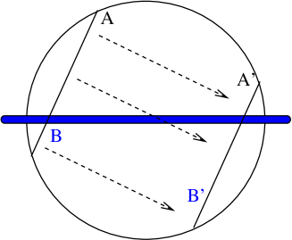
This is shown schematically in Fig. 21. Consider a sky map that is zero everywhere except on the GP, where it has some positive value. A circle AB that is translated with zero twist to the other side of the sky, i.e. to A’B’, fails to match the circle A’B’. B is close to the GP but B’ is not close to the GP, and A is far from the GP, while A’ is close to the GP. Keeping in mind that the sky here is , it is clear that a twist of is required so that the two points that intersected with the GP in the first matched circle again intersect the GP after the translation. In other words, the favoured twist angle is . This geometry applies for arbitrary circles, except for those nearly parallel or orthogonal to the GP. Hence, the signal shown in the lower panel of Fig. 20 is just what can be expected from a galactic signal, and does resemble our detected signal.
If the signal we found is caused by the Galaxy, then it is not due to the dominant part of the Galaxy signal, but rather to a more subtle aspect of the galactic signal which by chance has a PDS-like symmetry.
5.2 Modifications to the infinite flat model
Is there any modification to the simplest version of the infinite flat model, such as modelling our location in a local void (e.g. Inoue & Silk 2006) or other methods of attempting to explain the lack of large-scale power or the “Axis of Evil” (e.g. Land & Magueijo 2007, and references therein), that would explain a dodecahedrally symmetric pattern of twists by ? This could be possible, in principle, although in that case, the question of which model is preferred by Occam’s Razor would arise. This topic goes beyond the scope of this paper.
5.3 Is built into our method or software?
Could the results found here be somehow built into the geometrical, correlational, or other algorithmical aspects of our method, or be caused by one or more bugs in the software? Extensive cross-checking of different parts of the circles package indicates no sign of an error significant enough to create an artificial signal similar to the one found here. However, in principle, any moderately complex piece of software can always contain bugs.

As discussed in Sect. 5.1.1, analysis of the WMAP Q map gave a clear signal consistent with what is expected — an axisymmetric, nearly uniform distribution of preferred face centres and a strongly preferred phase of . However, this is clearly a very special situation with a very particular resulting twist phase . Here we describe a more general test. The principle is to create a simple, asymmetric pattern in six faces of a spherical dodecahedron, translate them to the opposite faces, and apply a twist. By construction, the cross-correlation should be very strong for this twist. In general, it should be weak for other twists. The MCMC method is then used to try to detect the preferred twist.
Some experimentation has indicated that the simplest test patterns are not necessarily sufficient to yield a convergent solution in 5-parameter space, since it is easy to induce false matches due to various periodicities between “adjacent” copies of the pattern. The function should be, in general, circularly asymmetric around each face centre so that only one favoured twist can be found. In the real Universe, it could happen that it is more difficult to find a single solution than in this artificial case. However, the result found in the WMAP data was that a single solution does indeed dominate. What is important to test is whether an artificial signal can lead to a strong, unique false detection.
The test pattern we adopted is
| (43) |
where and are both in degrees. This is a smooth, moderately sinusoidal, asymmetric function of and , used for all pixels within 31.7∘ of the centre of a dodecahedral face, i.e. within a disc approximately touching the edges of the pentagonal border. These pixels are then copied by a translation to the opposite face and rotated by a twist of .
There is only a trivial algorithmic difference between stepping in all five parameters or stepping in a single parameter. In this way, we can test most aspects of our method and software, as indicated in Sects 3.5 and 3.6, in particular, the estimates of the correlation functions, the calculation of the probability estimator defined in Eq. (36), and the basic MCMC functionality, by starting our simulated maps at the correct input values for the simulated map and holding these constant, while starting at an arbitrary phase unrelated to the input value of the simulated map.
If something is wrong with the correlation function estimation, the probability estimator defined in Eq. (36) or the basic MCMC functionality, or if a phase is somehow accidentally built into the software, then this should be revealed by toy simulations of this type. Figure 22 compares input and output values of based on 20 MCMC chains, each of 6000 steps. Each input toy map is generated for a random point , and the chain is started at the same position but a random twist . Since the artificial maps contain matching 31.7∘ discs, we restrict the circle size in the MCMC chains to .
Estimates of are based on steps 1001 to 6000 (i.e. removing a burn-in of 1000 steps) of a simulation, using a minimum probability requirement of as for the analysis on real data. The mean of the differences for the 20 chains is with a standard error in the mean of . Clearly, the input and output twists are statistically close to equal. Moreover, there is no sign that either of are favoured due to either an intrinsic error in our method or to a software error. If the correlation function estimates, “probability” estimator, and general MCMC functionality contain any hidden errors, then these do not explain our estimate of .
5.4 Is the expected distribution of uniform?
If the simply connected model is assumed, then the spatial auto-correlation on large scales could conceivably be used to model the expected cross-correlations, though this would probably neither be easy nor free of model-dependent assumptions.
For a fixed circle radius, as increases from zero to , the separation between identified points increases. Thus, if the autocorrelation were monotonically decreasing as separation increased, then higher values of would imply lower correlations.
However, for circle radii , which constitute almost all the points shown in Fig. 8, the separation (assuming simple connectedness) between opposite circles is a minimum of times an SLS radius, i.e. a minimum of 13.4 Gpc. If the auto-correlation function is reasonably isotropic, then over the range , the cross-correlation will sample Figure 1 shows that this function is approximately flat and close to zero, at least relative to the correlations at
The largest circle radii we considered here are those with . This gives a minimum of one SLS radius (9.5 Gpc) separating a pair of points under the simply connected assumption, which is approximately the separation at which becomes flat and approximately zero. Hence, if the auto-correlation estimated under the simply connected assumption and shown in Fig. 1 is approximately correct, then the expected distribution of for the range of circle sizes considered here should be close to uniform.
Independently of trying to explain our result in terms of a simply connected model, what other evidence could support the PDS interpretation?
5.5 Can this solution be confirmed on smaller scales?
Probably the biggest open question raised from the present work is the nature of the signal at smaller length/angular scales: Gpc or . Investigating this would require much smaller Markov chain steps than we have used here.
To have our Markov chains converge in a reasonably short time but also have them start at arbitrary positions in parameter space, we defined a 10∘ width Gaussian for stepping between points. Now that the globally optimal point in parameter space has been found, chains with a narrower width, and/or a stricter “probability” function for deciding how probable it is that a point in parameter space corresponds to a correct solution, could be used to find an optimal point with higher angular resolution, by starting from our present solution as an approximate solution, rather than starting from arbitrary points in parameter space.
However, if our solution is physically correct, then while there is no reason why the intrinsic density-density cross-correlation at sub-gigaparsec scales should differ from the density-density auto-correlation, we can expect some differences in temperature-temperature correlations due to various projection effects: both the Doppler effect and the integrated Sachs-Wolfe effect (ISW) should cause some differences between the two functions when correlating temperature fluctuations. Another complication on small scales, as Aurich et al. (2006) have shown, is that the WMAP ILC map has a lack of signal on these scales.
Furthermore, could the stronger cross-correlation for our PDS solution at around 3–8 Gpc relative to the auto-correlation be explained by ISW dampening of the auto-correlation on these scales? Since the cross-correlation temperatures corresponding to these cross-correlations are observed, in general, at widely different angles, they are less likely to be foregrounded by the same ISW fluctuation, so this seems possible at least qualitatively.
A practical problem in extending the present method to smaller scales is the need to use enough pairs of points on the SLS for which is “small”. For a given, finite number of points , there are fewer and fewer pairs of points separated by smaller and smaller separations.
As explained in Sect. 3.5, we used points distributed uniformly on the sphere. In fact, a larger number of points are generated when a galactic contamination mask is used. To avoid any chance of bias, the points are generated uniformly, excluding those falling within the mask, until the required number of points have been obtained. Excluding distantly separated pairs of points, where the distance is the minimum of for the 12 holonomy transformations , is a heavy computational task equivalent to making the main calculation loop needed for correlation function estimation.
Testing of smaller scales therefore requires considerably more pairs of points, and this would seem to scale as , increasing the calculation time proportionally. Improvements to this scaling using geometrical arguments would likely be complex and would risk inducing an ambiguity as to whether the new results are due to the non-uniform distribution of the points or to the intrinsic properties of the data.
5.6 Are the “secondary” and “tertiary” solutions explainable as PDS harmonics (eigenmodes)?
5.7 Is this solution compatible with other PDS analyses of the WMAP data?
The Roukema et al. (2004) “hint” of a solution was based on looking for identified circles, so, as noted above in Eq. (5), was based on using a much smaller part of the available signal to search for a candidate favoured PDS orientation. Key et al. (2007) and Lew & Roukema (2008) agree that the solution is a local maximum in the parameter space, but that it is not statistically significant. Using the greater amount of information available from the cross-correlation at separations going up to Gpc rather than just , the results presented in Sect. 4.4 agree that the Roukema et al. (2004) PDS solution is not globally favoured by the data. Moreover, MCMC chains starting at that solution move towards and converge towards the solution found with the present method.
One way of comparing with other PDS analyses, which use quite different methodologies to analyse the WMAP data, is to consider estimates of the total density parameter . Luminet et al. (2003) initially favoured an estimate of , but in more recent work using many more eigenmodes of the PDS, they favour (for ) by requiring maximal suppression of the quadrupole (Caillerie et al. 2007). In analyses based on WMAP first-year estimates, Aurich et al. (2005b) found , and using a combined match circles method, Aurich et al. (2006) favoured (for ).
Are these consistent with our solution? The total density parameter relates tightly to the circle radius , with some dependence on , e.g. Fig. 2 of Roukema et al. (2004) or Fig. 10 of Aurich et al. (2005b). The estimates (for ) and (for ) correspond to and respectively. Gundermann (2005) also found (for ) as one of his two solutions; this corresponds to .
As discussed in Sect. 4.2, the “matched discs” interpretation (Fig. 9) of Fig. 8 would imply a true matched circle radius of 30–40∘. This is clearly compatible with the Aurich et al. (2006) estimate, and possibly compatible with the Caillerie et al. (2007) and Gundermann (2005) estimates. Clearly, a variety of different methods, either requiring suppression of large-scale power (other work) or maximising large angular scale correlations in a PDS-like symmetry (our work), and either with the in-built constraint that the twist is (other work) or without that constraint (our work), seem to converge on similar results.
6 Conclusion
It seems hard to avoid the conclusion that cross-correlations of temperature fluctuations on would-be adjacent copies of the SLS, which are distant from one another and are (on average) very weakly correlated according to the WMAP 3-year observations, (i) imply a highly cross-correlated “generalised” Poincaré dodecahedral space symmetry (Figs 5–7, Table 1) at which these on-average uncorrelated fluctuations happen to be well-correlated with one another (Fig. 11), and, moreover, (ii) this favoured solution is dominated by a signal whose twist phase lies within a few degrees of one of the two twist phases necessary for a valid PDS model (Table 2).
These two successful predictions of the PDS model follow the WMAP confirmation of the generic prediction of small universe models, a power cutoff in structure statistics on large scales, and the solution appears to be consistent with quite different PDS analyses of the WMAP data.
Do we really live in a Poincaré dodecahedral space? Further constraints either for or against the model are certainly still needed, but the evidence in favour of a PDS-like signal in the WMAP data does seem to be accumulating.
Acknowledgments
Helpful comments from Bartosz Lew were greatly appreciated. Use of the Nicolaus Copernicus Astronomical Center (Toruń) computer cluster is gratefully acknowledged. Use was made of the WMAP data http://lambda.gsfc.nasa.gov/product/ and of the Centre de Données astronomiques de Strasbourg http://cdsads.u-strasbg.fr.
References
- (1) Aurich, R., Lustig, S., & Steiner, F. 2005a, ClassQuantGra, 22, 3443, astro-ph/0504656
- (2) Aurich, R., Lustig, S., & Steiner, F. 2005b, ClassQuantGra, 22, 2061, astro-ph/0412569
- Aurich, Lustig, & Steiner (2006) Aurich, R., Lustig, S., & Steiner, F. 2006, MNRAS, 369, 240, astro-ph/0510847
- Blanlœil & Roukema (2000) Blanlœil, V., & Roukema, B. F., eds. 2000, “Cosmological Topology in Paris 1998” (Paris: Blanlœil & Roukema), astro-ph/0010170
- Caillerie, Lachièze-Rey, Luminet, Lehoucq, Riazuelo, & Weeks (2007) Caillerie, S., Lachièze-Rey, M., Luminet, J. ., et al. 2007, A&A, 476, 691, 0705.0217v2
- Cornish, Spergel, & Starkman (1996) Cornish, N. J., Spergel, D. N., & Starkman, G. D. 1996, ArXiv Gen.Rel. & Quant.Cosm. e-prints, gr-qc/9602039
- Cornish, Spergel, & Starkman (1998) Cornish, N. J., Spergel, D. N., & Starkman, G. D. 1998, ClassQuantGra, 15, 2657
- Gausmann, Lehoucq, Luminet, Uzan, & Weeks (2001) Gausmann, E., Lehoucq, R., Luminet, J.-P., Uzan, J.-P., & Weeks, J. 2001, ClassQuantGra, 18, 5155, gr-qc/0106033
- Gundermann (2005) Gundermann, J. 2005, arXiv preprints, astro-ph/0503014
- Inoue & Silk (2006) Inoue, K. T., & Silk, J. 2006, ApJ, 648, 23, astro-ph/0602478
- Key, Cornish, Spergel, & Starkman (2007) Key, J. S., Cornish, N. J., Spergel, D. N., & Starkman, G. D. 2007, Phys. Rev. D, 75, 084034, astro-ph/0604616
- Lachièze-Rey & Luminet (1995) Lachièze-Rey, M., & Luminet, J. 1995, Phys. Rep, 254, 135, gr-qc/9605010
- Lambert (1772) Lambert, J. 1772, Anmerkungen und Zusätze zur Entwerfung der Land und Himmelscharten. In Beiträge zum Gebrauche der Mathematik und deren Anwendung, pt. 3, sec. 6. (English translation: Notes and Comments on the Composition of Terrestrial and Celestial Maps, Ann Arbor, University of Michigan 1972)
- Land & Magueijo (2007) Land, K., & Magueijo, J. 2007, MNRAS, 378, 153, arXiv:astro-ph/0611518
- Lehoucq, Weeks, Uzan, Gausmann, & Luminet (2002) Lehoucq, R., Weeks, J., Uzan, J.-P., Gausmann, E., & Luminet, J.-P. 2002, ClassQuantGra, 19, 4683, gr-qc/0205009
- Lew & Roukema (2008) Lew, B., & Roukema, B. F. 2008, A&A, 482, 747, 0801.1358
- Luminet & Roukema (1999) Luminet, J., & Roukema, B. F. 1999, in NATO ASIC Proc. 541: Theoretical and Observational Cosmology, 117, astro-ph/9901364
- Luminet, Weeks, Riazuelo, Lehoucq, & Uzan (2003) Luminet, J., Weeks, J. R., Riazuelo, A., Lehoucq, R., & Uzan, J. 2003, Nature, 425, 593, astro-ph/0310253
- Luminet (1998) Luminet, J.-P. 1998, Acta Cosmologica, XXIV-1, 105, gr-qc/9804006
- Neal (1993) Neal, R. 1993, Probabilistic Inference Using Markov Chain Monte Carlo Methods (Technical Report CRG-TR-93-1) [http://omega.albany.edu:8008/neal.pdf] (Department of Computer Science, University of Toronto: Toronto)
- Rebouças & Gomero (2004) Rebouças, M. J., & Gomero, G. I. 2004, Braz. J. Phys., 34, 1358, astro-ph/0402324
- Riazuelo, Weeks, Uzan, Lehoucq, & Luminet (2004) Riazuelo, A., Weeks, J., Uzan, J., Lehoucq, R., & Luminet, J. 2004, Phys. Rev. D, 69, 103518, astro-ph/0311314
- Roukema (2000) Roukema, B. F. 2000, Bull. Astr. Soc. India, 28, 483, astro-ph/0010185
- Roukema (2001) Roukema, B. F. 2001, MNRAS, 325, 138, astro-ph/0102099
- Roukema (2002) Roukema, B. F. 2002, in Marcel Grossmann IX Conference on General Relativity, eds V.G. Gurzadyan, R.T. Jantzen and R. Ruffini, World Scientific, Singapore, p. 1937, astro-ph/0010189
- Roukema (2005) Roukema, B. F. 2005, A&A, 439, 479, astro-ph/0409694
- Roukema, Bajtlik, Biesiada, Szaniewska, & Jurkiewicz (2007) Roukema, B. F., Bajtlik, S., Biesiada, M., Szaniewska, A., & Jurkiewicz, H. 2007, A&A, 463, 861, astro-ph/0602159
- Roukema, Lew, Cechowska, Marecki, & Bajtlik (2004) Roukema, B. F., Lew, B., Cechowska, M., Marecki, A., & Bajtlik, S. 2004, A&A, 423, 821, astro-ph/0402608
- Schwarzschild (1900) Schwarzschild, K. 1900, Vier.d.Astr.Gess, 35, 337
- Schwarzschild (1998) Schwarzschild, K. 1998, ClassQuantGra, 15, 2539
- Spergel, Bean, Doré, Nolta, Bennett, Hinshaw, Jarosik, Komatsu, Page, Peiris, Verde, Barnes, Halpern, Hill, Kogut, & et al. (2007) Spergel, D. N., Bean, R., Doré, O., et al. 2007, ApJS, 170, 377, astro-ph/0603449
- Spergel, Verde, Peiris, Komatsu, Nolta, Bennett, Halpern, Hinshaw, Jarosik, Kogut, Limon, Meyer, Page, Tucker, Weiland, Wollack, & Wright (2003) Spergel, D. N., Verde, L., Peiris, H. V., et al. 2003, ApJS, 148, 175, astro-ph/0302209
- Starkman (1998) Starkman, G. D. 1998, ClassQuantGra, 15, 2529
- Starobinsky (1993) Starobinsky, A. A. 1993, Journal of Experimental and Theoretical Physics Letters, 57, 622
- Stevens, Scott, & Silk (1993) Stevens, D., Scott, D., & Silk, J. 1993, Physical Review Letters, 71, 20
- Tegmark, de Oliveira-Costa, & Hamilton (2003) Tegmark, M., de Oliveira-Costa, A., & Hamilton, A. 2003, Phys. Rev. D, 68, 123523, astro-ph/0302496
- Uzan, Lehoucq, & Luminet (1999) Uzan, J.-P., Lehoucq, R., & Luminet, J.-P. 1999, in Proc. of the XIXth Texas meeting, Paris 14–18 December 1998, Eds. E. Aubourg, T. Montmerle, J. Paul and P. Peter, article no 04/25, gr-qc/0005128
- Weeks (2001) Weeks, J. 2001, The Shape of Space (2nd edition) (Manhattan: Marcel Dekker)
- Weinberg (1972) Weinberg, S. 1972, Gravitation and cosmology: Principles and applications of the general theory of relativity (New York: Wiley)