Study on $N\bar{N}$ $S$-wave Elastic Cross Section and Possible Bound States Within a Constituent Quark Model

Abstract

In the framework of a chiral constituent quark model, considering the contributions of $\pi$ annihilation and one-gluon annihilation, the proton-antiproton $S$-wave elastic scattering cross section experimental data can be reproduced by adjusting properly one-gluon annihilation coupling constant. Meanwhile, using the fixed model parameter, we do a dynamical calculation for all possible $S$-wave nucleon-antinucleon states, the results show that, there is no $S$-wave bound state as indicated by a strong enhancement at threshold of $p\bar{p}$ in $J/\psi$ and $B$ decays.

I introduction

Theoretical studies of baryon-antibaryon bound states date back to the proposal of Fermi and Yang fermi to make the pion with a nucleon-antinucleon pair. The traditional $N\bar{N}$ interaction studies, such as boundary condition model lomon , optical model cbdover and coupled-channel models liu , emphasized on the handling of the short-range part of $N\bar{N}$ interaction, and for the long range part they are quite similar. The extensive and excellent reviews are given in Ref.richard . Although the agreement with scattering experimental data is obtained, from the quantum chromodynamics (QCD) point of view it is hard to image that a hadronic picture can be applied to such a short-range where hadrons are “overlapped” and the internal structure of hadrons must be considered.

A possible way out is to start from QCD, the fundamental strong interaction theory. Namely we should start with quark-gluon degree of freedom, rather than the meson-baryon picture. QCD has been already proved to be the right theory at high energy. At low energy, because of the non-perturbative nature of QCD, one has to rely on effective theories and/or QCD-inspired models to get some insight into the phenomena of the hadronic world. The constituent quark model constituent1 ; constituent2 ; constituent3 ; constituent4 is one of them. It has been successful in describing hadron spectrum, the baryon-baryon interactions and the bound state of two baryons, the deuteron. Therefore, extending the constituent quark model to $N\bar{N}$ study is an interesting practice.

The early studies in the traditional meson exchange framework found that, if neglecting annihilation channels, many bound states might be formed, while annihilation effects were included, the binding force decreased and some bound states were washed outdover . Therefore, how to take into account the effect of annihilation in an unified framework is important. We attempt to include the contributions of the annihilations of a $q\bar{q}$ pair into meson or into gluon in an unified manner, besides including $\pi$, $\sigma$ and gluon exchange in the constituent quark model. In order to keep the model well-describing baryon spectrum and $NN$ scattering data, all of the model parameters have been fixed as much possible as those fixed in $NN$ interaction and baryon spectrum.

Perturbative QCD calculation showed that the gluon running coupling constant decreasing with the increasing of momentum transfer. Here we vary gluon annihilation coupling constant $\alpha^{\prime}_{s}$ to see if the proton-antiproton $S$-wave elastic cross section experimental dataexperiment can be well reproduced. For comparison, the case of ignoring the contributions of $\pi$ annihilation is also computed.

The BES collaboration in the radiative decay $J/\Psi\rightarrow\gamma p\bar{p}$ observed a sharp enhancement at threshold in the $p\bar{p}$ invariant mass spectrum bes . They tried to fit the enhancement by means of a $S$-wave Breit-Wigner resonance, and obtained the resultant mass peak below threshold. Belle also reported they observed an enhancement in the $p\bar{p}$ invariant mass distribution near the threshold in the decays $B^{+}\rightarrow K^{+}p\bar{p}$ and $B^{0}\rightarrow D^{0}p\bar{p}$ Belle . Many interpretations rosner ; zou ; datta ; he on the observation were suggested. Here we apply the constituent quark model constrained by baryon spectrum and $NN$ interaction and in addition considering the contribution of annihilation fixed by proton-antiproton $S$-wave elastic scattering cross section, to do a dynamical calculation for all possible $S$-wave nucleon-antinucleon system to study if there is $p\bar{p}$ $S$-wave bound state.

The paper is organized as follows. Sec. II explains the model Hamiltonian, its parameters and the calculation method. Sec. III is the results and discussions.

II Hamiltonian, model parameters and calculation method

We take the chiral quark model used in the study of multi-quark system, which essentially is an effective theory on exchanges of Goldstone boson, scalar meson $\sigma$, as well as gluon between quarks, and extend it to include the antiquarks and the annihilation interaction, to study the nucleon-antinucleon system.

As the first step, here only $S$-wave states of the nucleon-antinucleon pair are considered, i.e., the total orbital angular momentum $L=0$, and we have $J=S$ (the total angular momentum comes from quark spin only).

We start from a Hamiltonian which was used by Salamanca group for NN interactionconstituent3 . It is one of the chiral quark model with only $\pi$ and $\sigma$ mesons. The quark-meson coupling constant $\alpha_{ch}$ is fixed by $g^{2}_{NN\pi}/4\pi$

$$\frac{g^{2}_{ch}}{4\pi}=(\frac{3}{5})^{2}\frac{g^{2}_{NN\pi}}{4\pi}\frac{m^{2}_{q}}{M^{2}_{N}},~{}~{}~{}~{}\alpha_{ch}=\frac{g^{2}_{ch}}{4\pi}\frac{m^{2}_{\pi}}{4m^{2}_{u}}.$$

The quark mass $m_{q}$ and $\sigma$ meson mass $m_{\sigma}$ are taken to be 313 MeV and 3.421 fm^-1, respectively. Quark-gluon coupling constant $\alpha_{s}$ is determined by the $\Delta-N$ mass difference. The confinement strength, $a_{c}$ is obtained from nucleon stability condition. Parameters and the calculated deuteron properties are listed in Table I.

Table I. Model Parameters, deuteron properties. $\delta_{OGE}$, $\delta_{OPE}$ (MeV) are the contributions of gluon, $\pi$ exchanges to $\Delta-N$ mass difference, respectively.

$b$(fm)	$\alpha_{s}$	$\alpha_{ch}$	$\Lambda$(fm${}^{-1})$	$a_{c}$(MeV fm${}^{-2})$	$V_{0}$(MeV)	$\delta_{OGE}$	$\delta_{OPE}$	$B_{D}$(MeV)	$\sqrt{(}r^{2})$(fm)	$P_{D}$
0.518	0.485	0.027	4.2	46.938	-487.29	145.6	148	2.0	1.96	4.86

To extend model from $NN$ systems to $N\bar{N}$ systems, we have to take into account the annihilation contributions in addition to the scattering ones: the relevant scattering and annihilation Feynman diagrams are shown in Fig.1 and Fig.2.

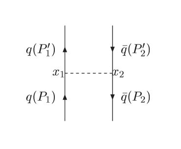
Figure 1: The exchange diagram between quark and antiquark

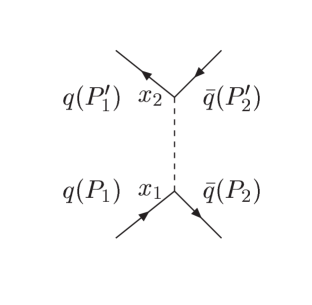
Figure 2: The annihilation diagram between quark and antiquark

Taking $\pi$ exchange as an example (in orbit and spin space), the T-matrix of $\pi$ exchange diagram between quark and antiquark can be written as

$$\bar{u}(p^{\prime}_{1},s^{\prime}_{1})\gamma^{5}u(p_{1},s_{1})\frac{-F^{2}(\vec{q}^{2})}{q^{2}+m^{2}_{\pi}}g^{2}_{ch}\bar{v}(p_{2},s_{2})\gamma^{5}v(p^{\prime}_{2},s^{\prime}_{2}),$$ (1)

here, a form factor $F(\vec{q}^{2})$ is assumed to be $(\Lambda^{2}/(\Lambda^{2}+\vec{q}^{2}))^{1/2}$. $p_{1},s_{1},p^{\prime}_{1},s^{\prime}_{1}$ are the four-vector momenta and spin z-projections of initial quark and final quark, respectively. $p_{2},s_{2},p^{\prime}_{2},s^{\prime}_{2}$ are the four-vector momenta and spin $z$-projections of initial antiquark and final antiquark, respectively. $u$ and $v$ are assumed to be free Dirac spinors for quarks and antiquarks, respectively, $m_{\pi}$ is the $\pi$ mass.

Similarly, T-matrix of $\pi$ annihilation diagram can be written as

$$-\bar{u}(p^{\prime}_{1},s^{\prime}_{1})\gamma^{5}v(p^{\prime}_{2},s^{\prime}_{2})\frac{-1}{q^{2}+m^{2}_{\pi}}g^{2}_{ch}\bar{v}(p_{2},s_{2})\gamma^{5}u(p_{1},s_{1})$$ (2)

using Fierz identities for Dirac matrices, a four-fermion matrix can be expressed as a linear superposition of other matrices with a changed sequence of spinors zong .

$$({\bar{a}}O_{i}b)({\bar{c}}O^{i}d)=\sum^{16}_{k=1}({\bar{a}}O_{k}d)({\bar{c}}O^{k}b)$$

Then we take the non-relativistic limit and transform the potential to space-time representation, we have

$$V^{{\pi}_{a}}_{q\bar{q}} = 4\pi\frac{g^{2}_{ch}}{4\pi}\frac{1}{m_{\pi}^{2}-(m_{1}+m_{2})^{2}}\delta(r)(-\frac{1}{2}-\frac{1}{2}\sigma_{i}\cdot\sigma_{j})(\frac{3}{2}-\frac{1}{2}\tau_{i}\cdot\tau_{j})(\frac{1}{3}+\frac{1}{2}\lambda_{i}\cdot\lambda_{j})~{}~{}~{}~{}~{}~{}$$ (3)

$$V^{\pi_{e}}_{q\bar{q}}(r) = -\frac{1}{12}\frac{g^{2}_{ch}}{4\pi}\frac{m^{2}_{\pi}}{m_{q_{i}}m_{q_{j}}}\left[\frac{e^{-m_{\pi}r}}{r}-\frac{\Lambda^{2}}{m^{2}_{\pi}}\frac{e^{-\Lambda r}}{r}\right]\frac{\Lambda^{2}}{\Lambda^{2}-m_{\pi}^{2}}\sigma_{i}\cdot\sigma_{j}\tau_{i}\cdot\tau_{j}$$ (4)

$$V^{g_{a}}_{q\bar{q}} = -\frac{4\pi\alpha^{\prime}_{s}}{(m_{1}+m_{2})^{2}}\delta(r)\frac{1}{4}(\frac{16}{9}-\frac{1}{3}\lambda^{c}_{i}\cdot\lambda^{c}_{j})(\frac{1}{2}+\frac{1}{2}\tau_{i}\cdot\tau_{j})(-\frac{3}{2}+\frac{1}{2}\sigma_{i}\cdot\sigma_{j})$$ (5)

$V^{\pi_{e}}_{q\bar{q}}$ and $V^{\pi_{a}}_{q\bar{q}}$ are the effective potential from $\pi$ exchanges and annihilation between quark and antiquark, respectively. $V^{g_{a}}_{q\bar{q}}$ are the effective potential from one gluon annihilation. Because here $N$ and $\bar{N}$ are both color singlet and there is no quark exchange between $N$ and $\bar{N}$, one gluon exchange between $N$ and $\bar{N}$ does not contribution at all.

Since we are taking into account the contributions of the lowest order to the $S$-wave at this step, under static approximation the contribution from $\sigma$ meson annihilation in the present case vanishes. The $\sigma$ exchange potential between quark and antiquark in the non-relativistic limit in coordinate space can been written as

$$V^{\sigma_{e}}_{q\bar{q}}(r) = -\frac{g^{2}_{ch}}{4\pi}\frac{\Lambda^{2}}{\Lambda^{2}-m_{\sigma}^{2}}\left[\frac{e^{-m_{\sigma}r}}{r}-\frac{e^{-\Lambda r}}{r}\right].$$ (6)

The detailed derivation of these effective potentials between quark and antiquark can be found in Ref.chang .

Therefore, the Hamiltonian of $N\bar{N}$ system is

$$H_{p\bar{p}} = \sum_{i=1}^{6}(m_{i}+\frac{p_{i}^{2}}{2m_{i}})-T_{CM}+\sum_{i>j=1}^{6}[V_{conf}(r_{ij})+V^{e}(r_{ij})+V^{a}_{q\bar{q}}(r_{ij})]$$

$$V^{e}(r_{ij}) = V^{\pi_{e}}_{qq,q\bar{q}}(r_{ij})+V^{\sigma_{e}}_{qq,q\bar{q}}(r_{ij})+V^{gluon_{e}}_{qq,q\bar{q}}(r_{ij})$$ (7)

$$V^{a}_{q\bar{q}}(r_{ij}) = V^{\pi_{a}}_{q\bar{q}}(r_{ij})+V^{\sigma_{a}}_{q\bar{q}}(r_{ij})+V^{g_{a}}_{q\bar{q}}(r_{ij})$$

$$V_{conf}(r_{ij}) = -a_{c}\lambda_{i}^{c}\cdot\lambda_{j}^{c}r_{ij}+V_{0}.$$

We should note that, in order to keep the model well-describing baryon spectrum and $NN$ scattering data, all of the model parameters related to $NN$ system are unchanged, only one parameter $\alpha^{\prime}_{s}$ connected with annihilation has been left to be adjusted.

We use Kohn-Hulthen-Kato variational method for bound and scattering problems in an unified frameworkkhk ; oka .
(i) for bound problem

Following the cluster model approach, the resonating group method (RGM) wave function is written as

$$\Psi_{LM}(\xi_{B_{1}},\xi_{B_{2}},\vec{R})={\cal A}[\phi_{B_{1}}(\xi_{B_{1}})\phi_{B_{2}}(\xi_{B_{2}})\chi(\vec{R})]$$

here $\vec{R}$ is the relative coordinate between the clusters of ${B_{1}}$ and ${B_{2}}$. $\cal A$ is the antisymmetrization operator but in fact there is no need for this antisymmetrization for $N\bar{N}$ system because $q$ and $\bar{q}$ can be treated as different particles. $\phi_{B_{1}}$ and $\phi_{B_{2}}$ are the internal wave functions of two quark clusters, $\chi(\vec{R})$ is relative motion wave function.

The relative motion wave function is expanded into partial waves

$$\chi(\vec{R}) = \sum_{L}\chi^{L}(R)Y^{LM}(\hat{R})=\sum_{L}\sum_{i=1}^{N}c_{i}^{L}\chi_{i}^{L}(R,S_{i})Y^{LM}(\hat{R})$$ (8)

with

$$\chi_{i}^{L}(R,S_{i})Y^{LM}(\hat{R}) = (\frac{3}{2\pi b^{2}})^{3/4}\int exp({-\frac{3}{4b^{2}}(\vec{R}-\vec{S}_{i})^{2}})Y^{*LM}(\hat{R})d\Omega_{R}Y^{LM}(\hat{S}_{i})d\Omega_{S_{i}}$$ (9)

$$= 4\pi(\frac{3}{2\pi b^{2}})^{3/4}exp({-\frac{3}{4b^{2}}(R^{2}+S_{i}^{2})})i_{L}(\frac{3}{2b^{2}}RS_{i})Y^{LM}(\hat{R})$$

where $i_{L}$ is the modified spherical Bessel function. In this paper, only $S$ wave ($L=0$) is taken into account.

Adding the center of mass motion, the wave function of six quarks can be written as the production of the single-particle orbital wave function with different reference centers, i.e.,

$$\Psi_{6q} = {\cal A}\sum_{L_{k}}\sum_{i=1}^{n}C_{{L_{k}},i}\int d\Omega_{S_{i}}\prod_{\alpha=1}^{3}\psi_{\alpha}(\vec{S_{i}})\prod_{\beta=4}^{6}\psi_{\beta}(-\vec{S_{i}})[[\Phi_{p}^{j_{1}f_{1}}\Phi_{\bar{p}}^{j_{2}f_{2}}]^{I,S}Y^{L}(\hat{S}_{i})]^{J}[\chi_{c}(B_{1})\chi_{c}(B_{2})]^{[\sigma]}~{}~{}~{}~{}~{}~{}$$ (10)

here $\psi_{\alpha}(\vec{S_{i}})$ and $\psi_{\beta}(-\vec{S_{i}})$ are the single-particle orbital wave function with different reference centers, $L_{k}$ is the coupled channels index.

Via the variation with respect to the relative motion wave function $\chi(R)$, the RGM equation

$$\int H(\vec{R},\vec{R}^{\prime})\chi(\vec{R}^{\prime})d\vec{R}^{\prime} = E\int N(\vec{R},\vec{R}^{\prime})\chi(\vec{R}^{\prime})d\vec{R}^{\prime}$$ (11)

becomes an algebraic eigenvalue equation

$$\sum_{j,{L_{k}^{\prime}}}C_{j,{L_{k}^{\prime}}}H^{L_{k},L_{k}^{\prime}}_{i,j} = E\sum_{j}C_{j,L_{k}}N^{L_{k}}_{i,j}.$$ (12)

where $N^{L_{k}}_{i,j}$ and $H^{L_{k},L_{k}^{\prime}}_{i,j}$ are the wave function overlaps and Hamiltonian matrix elements, respectively.
(ii) for scattering problem

The wave function of the relative motion is expanded by

$$\chi(\vec{R}) = \sum_{L}\chi^{L}(R)Y^{LM}(\hat{R})=\sum_{L}\sum_{i=0}^{n}c_{i}^{L}\tilde{\chi}_{i}^{L}(R,S_{i})Y^{LM}(\hat{R})$$ (13)

here

$$\tilde{\chi}_{i}^{L}(R,S_{i}) = \left\{\begin{array}[]{cc}\alpha_{i}\chi_{i}^{L}(R,S_{i})&R<R_{c}\\ (h_{L}^{(-)}(kR)-s_{i}h_{L}^{(+)}(kR))kR&R>R_{c}\\ \end{array}\right.$$ (16)

with

$$\chi_{i}^{L}(R,S_{i})=\frac{u_{i}^{L}(R,S_{i})}{R} = 4\pi(\frac{3}{2\pi b^{2}})^{3/4}exp[{-\frac{3}{4b^{2}}(R^{2}+S_{i}^{2})}]i_{L}(\frac{3}{2b^{2}}RS_{i})$$ (17)

where $i_{L}$ is the modified spherical Bessel function. $h_{L}^{(\pm)}$ is the $L$-th spherical Hankel function, $k=\sqrt{(}2\mu E_{rel})$.

The constants $\alpha_{i}$ and $s_{i}$ are determined by the condition that the relative motion wave function for $R<R_{c}$ and $R>R_{c}$ smoothly connect at $R=R_{c}$.

Using the normalization condition $c_{0}=1-\sum_{i=1}^{n}c_{i}$ and varying with respect to parameters $c_{i}~{}(i=1,...,n)$, we have

$$([u_{i}-u_{0}]\L_{L}u_{t})=0,i=1,...,n$$

with a symbol $(f\L_{L}g)$ by

$$(f\L_{L}g)=\int_{0}^{\infty}\int_{0}^{\infty}f(R)\L_{L}(R,R^{\prime})g(R^{\prime})dRdR^{\prime}$$

,

$$\L_{L}(R,R^{\prime})=\int[\phi^{+}_{A}(\xi_{A})\phi^{+}_{B}(\xi_{B})u_{i}^{L}(R)Y^{*}_{LM}(\hat{R})](H-E){\cal A}[\phi_{A}(\xi_{A})\phi_{B}(\xi_{B})u_{j}^{L}(R)Y_{LM}(\hat{R})],$$

then we have the n linear equations for the $c_{i}$’s,

$$\sum_{j=1}^{n}\L_{ij}c_{j}=M_{i}$$ (18)

where

$$\L_{ij} = K_{ij}-K_{i0}-K_{0j}+K_{00},M_{i}=K_{00}-K_{i0}$$ (19)

with

$$K_{ij} = (u_{i}\L_{L}u_{j})$$ (20)

The final phase shift is

$$s_{st} = s_{t}+i\alpha\sum_{i=0}^{n}K_{0i}c_{i}$$ (21)

here $\alpha=\mu/k$, $\mu$ is the reduced mass. The difference $s_{t}-s_{st}$ is a good measure to check the accuracy of the calculation. In order to calculation $K_{ij}$ (term(18)) as analytically as possible, there is a very useful skill mentioned in Ref.khk .

III Results and Discussions

There are four possible states for an S-wave nucleon-antinucleon systems with different isospin and total angular momentum J respectively. They are $IJ^{PC}=11^{--}$, $10^{-+}$, $01^{--}$, $00^{-+}$. Since running coupling constant would change with momentum transfer, here we adjust gluon annihilation coupling constant $\alpha^{\prime}_{s}$ from being smaller than exchange coupling constant $\alpha_{s}$ to larger than $\alpha_{s}$.

In experiment one measures the spin-averaged scattering amplitudes, and the elastic scattering amplitude is the sum of the isospin $I=0$ and $I=1$ amplitudes with equal weights. According these, we calculated the total proton-antiproton elastic cross sections, and compare it with experimental data.

We calculated $p\bar{p}$ $S$-wave elastic cross section including $\pi$ annihilation and gluon annihilation with different gluon annihilation coupling constant $\alpha^{\prime}_{s}$, the results are shown in Fig.3. We found that, if we let $\alpha^{\prime}_{s}=0$ (i.e.,we did not take into account the effect of gluon annihilation) the cross section would be very larger than experimental data. It implies that, if excluding the gluon annihilation process, $N\bar{N}$ system is more attractive than $NN$ system and many bound states might be formed, which is consistent with the results in Ref.dover ; buck . When we add the contribution of gluon annihilation, with a gradual increasing $\alpha^{\prime}_{s}$, the cross section will decrease quickly, especially in the low energy region. And the larger $\alpha^{\prime}_{s}$ is, the smoother the change of cross section with the scattering energy is. If we choose $\alpha^{\prime}_{s}$ equal to $\alpha_{s}$, the cross section will be below the experimental data. When we choose $\alpha^{\prime}_{s}$ is about the one third of gluon exchange coupling constant $\alpha_{s}$ ($\alpha^{\prime}_{s}=\alpha_{s}/3$), the cross section became close to experimental data, the difference between theoretical cross section and experimental one would not more than 5 mb.

Fig.3 proton-antiproton elastic cross sections, including $\pi$ annihilation and one-gluon annihilation with different coupling constants. The full squares show experimental data of total elastic cross section. The open squares are that of $S$-wave componentexperiment .

Fig.4 Same as Fig.3 but $\pi$ annihilation excluded.

Fig.3 proton-antiproton elastic cross sections, including $\pi$ annihilation and one-gluon annihilation with different coupling constants. The full squares show experimental data of total elastic cross section. The open squares are that of $S$-wave component experiment . Since annihilation process would happen at short range, and $\pi$ term might play an important role only at long range, so we do a calculation by excluding the $\pi$ annihilation term. Fig.4 shows the $p\bar{p}$ cross section with the different $\alpha^{\prime}_{s}$ in the case of excluding the contribution of $\pi$ annihilation. We found that, larger $\alpha^{\prime}_{s}$ corresponds to smaller cross section. In order to reproduce $p\bar{p}$ $S$-wave elastic cross section, the effective gluon annihilation coupling constant $\alpha^{\prime}_{s}$ should increase to compensate for the absence of $\pi$ annihilation. The proper value is $\alpha^{\prime}_{s}$=$\alpha_{s}/0.9$, which is very close to gluon exchange coupling constant.

The above results implies that both gluon annihilation and $\pi$ annihilation provide effective repulsion, which would decrease the $S$-wave cross section. By adjusting the strength of annihilation term properly, proton-antiproton $S$-wave cross section experimental data can be reproduced no matter the $\pi$ annihilation is included or not.

Taking $\alpha^{\prime}_{s}=\alpha_{s}/3$ and $\alpha^{\prime}_{s}=\alpha_{s}/0.9$ as examples, we give the contributions of different spin and isospin components to the total cross section in Fig.5 and Fig.6 for including and excluding $\pi$ annihilation, respectively. The results show that, the contribution of $IJ=00$ channel is always very small no matter the $\pi$ annihilation is included or not; the $IJ=01$ channel contribution to cross section is larger than $IJ=10$ channel when $\pi$ annihilation is included; while the former contribution is smaller than the latter if the $\pi$ annihilation is excluded; and with the increasing of scattering energy the difference between these two channels contributions are both decreasing in these two cases; For the case of including $\pi$ annihilation, the total cross section is close to the $IJ=11$ channel ones when scattering energy $E_{cm}$ is below 15 MeV and it will be close to $IJ=10$ channel ones when $E_{cm}$ is above 15 MeV. If excluding the contribution of $\pi$ annihilation, the total cross section is very close to $IJ=11$ channel in the whole energy range.

Fig.5 $S$-wave elastic cross sections with $\alpha^{\prime}_{s}=\alpha_{s}/3.0$ in the case of including $\pi$ annihilation, for channel $IJ=11,10,01,00$, respectively.

Fig.6 Same as Fig.5 for the case of excluding $\pi$ annihilation with $\alpha^{\prime}_{s}=\alpha_{s}/0.9$.

The effective potentials of $IJ=11,10,01,00$ channels are given in Fig.7 and Fig.8 corresponding to different annihilation coupling constants. From these figures we found that $IJ=00$ channel has very small intermediate attraction no matter what parameters are chosen, which is consistent with the results of cross section in Fig.5-6. The other three channels all have attraction to some extent. Excluding the contribution of $\pi$ annihilation there will be more attraction left in the other three channels, and the minimum values of potential are all at the separation of  1.0 fm.

The BES collaboration in the radiative decay $J/\psi\rightarrow\gamma p\bar{p}$ observed a sharp enhancement at threshold in the $p\bar{p}$ invariant mass spectrumbes , and they obtained the mass peak below the threshold of $p\bar{p}$. The above effective potentials give qualitative information only, in order to see whether there is a $p\bar{p}$ bound state, we do a dynamical calculation. Taking into account the contribution of annihilation and using the model parameters (in Fig.5-6) determined by proton-antiproton S-wave elastic scattering cross section, we solve RGM equation for all possible S-wave nucleon-antinucleon states, to see if there is $p\bar{p}$ S-wave bound state. Here, we use 10 basis wave functions to expand the wave function of the relative motion, the boundary point is at 5.8 fm. We find that, although the four possible channels with different isospin and spin quantum numbers all have intermediate range attraction ( from several Mev to about 50 MeV), there is no bound state in dynamical calculation. Moreover, there is no resonant state below the system mass of 3.9 GeV in our calculation. That is to say, if we determine the model parameter of quark-antiquark annihilation by fitting proton-antiproton S-wave elastic cross section experimental data, our model does not support a tight bound state claimed by BES and Belle experimental groups.

Fig.7 Proton-antiproton effective potential with $\alpha^{\prime}_{s}=\alpha_{s}/3.0$, including $\pi$ annihilation, for channel $IJ=11,10,01,00$, respectively.

To sum up, in the framework of chiral quark model, adding the contribution of one gluon and $\pi$ annihilation, we can reproduce proton-antiproton $S$-wave elastic cross section experimental data by adjusting the coupling constant of gluon annihilation term. Using the model parameters determined by $p\bar{p}$ scattering cross section, our dynamical calculation for $N\bar{N}$ system with $IJ=11,10,01,00$, quantum numbers does not find an $S$-wave bound state.

Fig.8 Same as Fig.7 for excluding $\pi$ annihilation with $\alpha^{\prime}_{s}=\alpha_{s}/0.9$.

Obviously our conclusion of no $p\bar{p}$ bound state is based on the assumption that the chiral constituent quark model is suitable for $N\bar{N}$ system. Our conclusion is also based on the assumption that the multi $\pi$ channel coupling effect, which is possible within the chiral constituent quark model, can be neglected. In addition all of the hidden color channels coupling effects have been omitted. All of these effects should be studied further.

IV Acknowledgments

This work is supported by the NSFC under Contract No.10505006, 10375030 and 90503011. We would like to thank Dr. Chang Chao-hsi for his collaboration in developing this model.

References

- (1) E.Fermi and C.N.Yang, Phys.Rev.76,1739(1949).
-
(2)
H.Feshbach,E.Lomon, Ann.Phys.(N.Y.)29,19(1964).
R.L.Jaffe,F.E.Low, Phys.Rev.D19,2105(1979). - (3) C.B.Dover,J.-M.Richard, Phys.Rev.C21,1466(1980).
- (4) G.Q.Liu,F.Tabakin, Phys.Rev.C41,665(1990).
-
(5)
J.M.Richard, nucl-th/9909030;
E.Klempt, F.Bradamante, A.Martin and J.M.Richard, Phys.Rep.368,119(2002). - (6) Y.W.Yu, Z.Y.Zhang, P.N.Shen and L.R.Dai,phys.Rev.C52,1(1995).
- (7) Y.Fujiwara, C.Nakamoto and Y.Suzuki, Phys.Rev.Lett 76,2242(1996).
-
(8)
F.Fernandez, A.Valcarce, U.Staub and
A.Faessler, J.Phys.G19,2031(1993).
A.Valcarce, A.Buchmann, F.Fernandez, and A. Faessler, Phys.Rev.C50, 2246 (1994).
A.Valcarce, H.Garcilazo, F.Fernandez, P.Gonzalez, Rept.Prog.Phys. 68,965 (2005). -
(9)
F.Wang, G.H.Wu, L.J.Teng and T.Goldman,
Phys.Rev.Lett.69,2901(1992).
F.Wang, J.L. Ping, G.H. Wu, L.J. Teng and T. Goldman, Phys. Rev. C51, 3411 (1995).
G.H. Wu, J.L. Ping, L.J. Teng, F. Wang and T. Goldman, Nucl. Phys. A673, 279 (2000).
H.R.Pang, J.L.Ping, F.Wang, T.Goldman, Phys.Rev.C65,014003(2001),C69,065207(2004). - (10) C.B.Dover,et al., Phys.Rev.D17,1770 (1978);Phys.Rev.C43,379(1991).
- (11) W.Bruckner, B.Cujec, H.Dobbeling et al., Z.Phys.A339,367(1991).
- (12) J.Z.Bai, et al., BES Collaboration, Phys.Rev.Lett.91,022001(2003).
- (13) K.Abe, et al., Belle collaboration, Phys. Rev. Lett. 88, 181803 (2002), 89, 151802 (2002).
- (14) J.L.Rosner, Phys.Rev. D68,014004(2003).
- (15) B.S.Zou and H.C.Chiang, Phys.Rev. D69,034004(2004).
- (16) A.Datta and P.J.O’Donnell, Phys.Lett. B567,273(2003).
- (17) Xiao-Gang He and Xue-Qian Li, hep-ph/0403191.
- (18) Hong-Shi Zong, Fan Wang, and Jia-Lun Ping, Commun.Theor.Phys.22,479(1994).
- (19) Chang Chao-Hsi and Pang Hou-rong, Commun.Theor.Phys.43,275(2005).
- (20) M.Kamimura,Sup.Prog.Theor.Phys.62,236(1977).
- (21) M.Oka and K.Yazaki, Prog.Theor.Phys.66,556(1981).
- (22) W.W.Buck, et al., Ann.Phys.121,47(1979).