Applications of distance between probability distributions to gravitational wave data analysis

Abstract

We present a definition of the distance between probability distributions. Our definition is based on the $L_{1}$ norm on space of probability measures. We compare our distance with the well-known Kullback-Leibler divergence and with the proper distance defined using the Fisher matrix as a metric on the parameter space. We consider using our notion of distance in several problems in gravitational wave data analysis: to place templates in the parameter space in searches for gravitational-wave signals, to assess quality of search templates, and to study the signal resolution.

1 Introduction

A number of long baseline interferometric gravitational wave detectors are working around the world: in the USA (LIGO project), in Italy (VIRGO project, a joint French-Italian collaboration), in Germany (GEO600 project), and in Japan (TAMA300 project). A network of resonant bar detectors continues its operation: in the USA (ALLEGRO detector) and in Italy (detectors AURIGA, NAUTILUS and EXPLORER (located in CERN near Geneva)). These detectors are collecting a large amount of data that are being currently analyzed. There is a proposed space borne detector LISA to be launched by NASA and ESA in the next decade. The quest for gravitational waves in the data requires optimal statistical methods and efficient numerical algorithms to search over very large parameter spaces [1, 2]. A standard method is the maximum likelihood detection method, which consists of searching for local maxima of the likelihood function with respect to the parameters [7]. Assuming Gaussian noise in the detector, the maximum likelihood method consists of correlating the data with templates defined over the parameter space. In this paper we introduce a new tool for data analysis - a distance between the probability density functions. This distance can be used to define the covering radius to design an optimal (with smallest number of nodes) grid in the parameter space. One can use the distance to determine the quality of the search templates - simplified models of the signal over a reduced parameter space. The distance can also be used to study the problem of signal resolution - a problem that occurs in the estimation of parameters of white dwarf binary systems in the data of planned space-borne detector LISA. This distance would play the same role in gravitational wave data analysis as the line element defined by the Fisher matrix interpreted as a Riemannian metric. However Fisher matrix is obtained as a Taylor expansion up to the second order term of the Kullback-Leibler divergence and therefore is only an approximation. Moreover the distance we introduce fulfills triangle inequality which is not true for Kullback-Leibler divergence from which the Fisher matrix is obtained. Moreover our distance can be defined for any probability densities, not only smooth and not only absolutely continuous with respect to each other.

In Section 2 we shall briefly review the problem of signal detection and parameter estimation. In Section 3 we shall motivate and introduce the $L_{1}$-norm distance between two probability density functions. We show that as a consequence of the triangle inequality, our distance is an appropriate tool in several data analysis problems. In Section 4 we shall review the Kullback-Leibler divergence. In Section 5 we shall calculate the $L_{1}$-norm and the Kullback-Leibler divergence in several cases important for applications, namely for the case of Gaussian probability density functions. In Section 6 we shall discuss applications of the $L_{1}$-norm to the problem of signal resolution, template placement and search template design for the simple case of a monochromatic signal. Section 7 concludes our paper.

2 Problem of signal detection and parameter estimation

2.1 Signal detection and parameter estimation in Gaussian noise

Suppose that we want to detect a known signal $s$ embedded in noise $n$. The signal detection problem can be posed as a hypothesis testing problem, where the null hypothesis is that the signal is absent, and the alternative hypothesis is that the signal is present. A solution to this problem has been found by Neyman and Pearson [8]. They have shown that, subject to a given false alarm probability, the test that maximizes the detection probability is the likelihood ratio test. Assuming that the noise is additive, the data time series $x(t)$ can be written as

$$x(t)=n(t)+s(t).$$ (1)

In addition if the noise is a zero-mean, stationary, and Gaussian random process, the log likelihood function is given by

$$\log\Lambda=(x|s)-\frac{1}{2}(s|s),$$ (2)

where the scalar product $(\,\cdot\,|\,\cdot\,)$ is defined by

$$(x|y):=4\Re\int^{\infty}_{0}\frac{\tilde{x}(f)\tilde{y}^{*}(f)}{\tilde{S}(f)}\,{\mathrm{d}}f.$$ (3)

In Eq. (3) $\Re$ denotes the real part of a complex expression, the tilde denotes the Fourier transform, the asterisk is complex conjugation, and $\tilde{S}$ is the one-sided spectral density of the noise in the detector. Equation (2) is called the Cameron-Martin formula [7]. From the Cameron-Martin formula we immediately see that the in the Gaussian case, the likelihood ratio test consists of correlating the data $x$ with the signal $s$ that is present in the noise and comparing the correlation to a threshold. Such a correlation $G=(x|s)$ is called the matched filter. The matched filter is a linear operation on the data.

An important quantity is the optimal signal-to-noise ratio $\rho$ defined by

$$\rho^{2}:=(s|s)=4\Re\int^{\infty}_{0}\frac{|\tilde{s}(f)|^{2}}{\tilde{S}(f)}\,{\mathrm{d}}f.$$ (4)

Since data $x$ are Gaussian and $G$ is linear in $x$, it has a normal probability density function. Probability density distributions $p_{0}$ and $p_{1}$ of correlation $G$ when respectively signal is absent and present are given by.

$$p_{0}(G) = \frac{1}{\sqrt{2\pi\rho^{2}}}\exp[-\frac{1}{2}\frac{G^{2}}{\rho^{2}}]$$ (5)

$$p_{1}(G) = \frac{1}{\sqrt{2\pi\rho^{2}}}\exp[-\frac{1}{2}\frac{(G-\rho^{2})^{2}}{\rho^{2}}].$$ (6)

Probability of false alarm $Q_{F}$ and of detection $Q_{D}$ are readily expressed in terms of error functions.

$$Q_{F} = \frac{1}{2}[1-erf(\frac{1}{\sqrt{2}}\frac{G_{o}}{\rho})]$$ (7)

$$Q_{D} = \frac{1}{2}[1-erf(\frac{1}{\sqrt{2}}(\frac{G_{o}}{\rho}-\rho))],$$ (8)

where $G_{o}$ is the threshold and the error function $erf$ is defined as

$$erf(x)=\frac{2}{\sqrt{\pi}}\int^{x}_{0}e^{-t^{2}}\,dt.$$ (9)

Thus to detect the signal we proceed as follows. We choose a certain value of the false alarm probability. From Eq. (7) we calculate the threshold $G_{o}$. We evaluate the correlation $G$. If $G$ is larger than the threshold $G_{o}$ we say that the signal is present. We see that in the Gaussian case, a single parameter – signal-to-noise ratio $\rho$ determines both probabilities – of false alarm and detection, and consequently the receiver’s operating characteristic. For a given false alarm probability, the greater the signal-to-noise ratio, the greater the probability of detection of the signal.

In general, we know the signal as a function of several unknown parameters $\theta$. Thus to detect the signal we also need to estimate its parameters. A convenient method is the maximum likelihood method, by which estimators are those values of the parameters that maximize the likelihood ratio. Thus the maximum likelihood estimators $\hat{\theta}$ of parameters $\theta$ are obtained by solving the set of equations

$$\frac{\partial\Lambda(\theta,x)}{\partial\theta_{i}}=0,$$ (10)

where $\theta_{i}$ is the $i$th parameter. The quality of any parameter estimation method can be assessed using the Fisher information matrix $\Gamma$ and the Cramèr - Rao bound [9]. The components of this matrix are defined by

$$\Gamma_{ij}:={\mathrm{E}}\bigg{[}\frac{\partial\log\Lambda}{\partial\theta_{i}}\frac{\partial\log\Lambda}{\partial\theta_{j}}\bigg{]}=-{\mathrm{E}}\bigg{[}\frac{\partial^{2}\log\Lambda}{\partial\theta_{i}\partial\theta_{j}}\bigg{]}.$$ (11)

The Cramèr-Rao bound states that for unbiased estimators, the covariance matrix of the estimators $C\geq\Gamma^{-1}$. (The inequality $A\geq B$ for matrices means that the matrix $A-B$ is nonnegative definite.) In the case of Gaussian noise, the formula for the Fisher matrix takes the form

$$\Gamma_{ij}=(\frac{\partial s(\theta)}{\partial\theta_{i}}|\frac{\partial s(\theta)}{\partial\theta_{j}}),$$ (12)

where the scalar product $(\,\cdot\,|\,\cdot\,)$ is given by Eq. (3).

2.2 The case of a monochromatic signal

Let us consider an application of the maximum likelihood estimation method to the case of a simple signal - a monochromatic signal. The monochromatic signal depends on three parameters: amplitude $A_{o}$, phase $\phi_{o}$, and angular frequency $\omega_{o}$, and it has the form

$$s=A_{o}\cos(\omega_{o}t-\phi_{o}).$$ (13)

Let us rewrite the signal (13) as

$$s=A_{c}\cos(\omega_{o}t)+A_{s}\sin(\omega_{o}t),$$ (14)

where

$$A_{c} = A_{o}\cos\phi_{o},$$ (15)

$$A_{s} = A_{o}\sin\phi_{o}.$$ (16)

Using Parseval’s theorem and assuming that the observation time $T$ is much longer than the period $2\pi/\omega_{o}$, we have

$$(\cos(\omega_{o}t)|\cos(\omega_{o}t)) \simeq (\sin(\omega_{o}t)|\sin(\omega_{o}t))\simeq\frac{T}{S_{o}},$$ (17)

$$(\cos(\omega_{o}t)|\sin(\omega_{o}t)) \simeq 0,$$ (18)

where $S_{o}$ is the one-sided spectral density of noise of the detector at frequency $\omega_{o}$. Thus the log likelihood ratio is approximately given by

$$\log\Lambda=2\frac{T}{S_{o}}[A_{c}<x\cos(\omega_{o}t)>+A_{s}<x\sin(\omega_{o}t)>-\frac{1}{2}(A_{c}^{2}+A_{s}^{2})],$$ (19)

where the operator $<\cdot>$ is defined as

$$<g(t)>=\frac{1}{T}\int^{T}_{0}g(t)\,dt=\int^{1}_{0}g(zT)\,dz,$$ (20)

where the last equation follows by introducing a dimensionless time variable $z=t/T$. The maximum likelihood estimators of $\hat{A}_{c}$ and $\hat{A}_{s}$ amplitudes $A_{c}$ and $A_{s}$ can be obtained in a closed analytic form by solving the set of the following two linear equations:

$$<x\cos(\omega_{o}t)>-A_{c}=0,$$ (21)

$$<x\cos(\omega_{o}t)>-A_{s}=0.$$ (22)

We have

$$\hat{A}_{c}=<x\cos(\omega_{o}t)>,$$ (23)

$$\hat{A}_{s}=<x\sin(\omega_{o}t)>.$$

By substituting the maximum likelihood estimators of amplitudes into the log likelihood ratio we get

$$\log\Lambda_{r}=\frac{T}{S_{o}}[<x\cos(\omega_{o}t)>^{2}+<x\sin(\omega_{o}t)>^{2}].$$ (24)

We shall denote the reduced likelihood ratio $\log\Lambda_{r}$ by ${\mathcal{F}}$ and we shall call it the ${\mathcal{F}}$ - statistic. The maximum likelihood estimators $\hat{\phi}_{o}$ and $\hat{A}_{o}$ of the phase and amplitude are given by

$$\hat{\phi}_{o} = \mbox{atan}[\frac{<x\sin(\omega_{o}t)>}{<x\cos(\omega_{o}t)>}],$$ (25)

$$\hat{A}_{o} = \sqrt{<x\cos(\omega_{o}t)>^{2}+<x\sin(\omega_{o}t)^{2}>}.$$ (26)

Thus to find the maximum likelihood estimators of parameters of the monochromatic signal, we first find the maximum of the ${\mathcal{F}}$ - statistic with respect to angular frequency, and the angular frequency $\hat{\omega}_{o}$ corresponding to the maximum of ${\mathcal{F}}$ is the maximum likelihood estimator of $\omega_{o}$. Then we use Eqs. (25) with $\omega_{o}=\hat{\omega}_{o}$ to find the maximum likelihood estimators of phase and amplitude. The maximum likelihood detection method consists of correlating the data $x$ with two filters $F_{c}=\cos(\omega_{o}t)$ and $F_{s}=\sin(\omega_{o}t)$. We easily see that the ${\mathcal{F}}$ - statistic is invariant with respect to the following transformation of the filters

$$\sin(\omega_{o}t)\rightarrow A_{F}\sin(\omega_{o}t+\phi_{F}),$$ (27)

$$\cos(\omega_{o}t)\rightarrow A_{F}\cos(\omega_{o}t+\phi_{F}),$$ (28)

where $A_{F}$ and $\phi_{F}$ are arbitrary constants.

With the above approximations, the signal-to-noise ratio $\rho$ and the Fisher matrix $\Gamma$ for the signal (13) are given by

$$\rho^{2} = A_{o}^{2}\frac{T}{S_{o}},$$ (29)

$$\Gamma_{ij} = \rho^{2}\left(\begin{array}[]{ccc}\frac{1}{A_{o}^{2}}&0&0\\ 0&1&\frac{T}{2}\\ 0&\frac{T}{2}&\frac{T^{2}}{3}\\ \end{array}\right),$$ (33)

where $i,j=(A_{o},\phi_{o},\omega_{o})$.

3 $L_{1}$-norm distance

3.1 Motivation

Let $I$ denote a probabilistic space of events $i\in I$; for the sake of clarity we will consider $I$ to be a set of finitely many elements in this initial discussion (generalization to continuous probabilistic spaces and measures will be commented upon later in this section). Let $p(i)$, $q(i)$ be two different probability distributions (strictly speaking: probabilistic measures) defined on $I$.

We propose to define the distance $d_{L}$ between two probability distributions $p$ and $q$ as

$$d_{L}=\frac{1}{2}\sum_{i\in I}\left|p(i)-q(i)\right|$$ (34)

where the sum is taken over the whole event space $I$.

The space of probability distributions with the above distance is a metric space because the distance fulfills all the axioms of a metric i.e. $d(p,q)=0$ if and only if $p=q$, $d(p,q)=d(q,p$) and the triangle equality holds: $d(p,q)+d(q,r)\geq d(p,r)$.

Remark: $d_{L}(p,q)\leq 1$ for any $p$, $q$; the maximal value is achieved if and only if $p$ and $q$ have disjoint supports, i.e. when for every $i\in I$ either $p=0$ or $q=0$.

We motivate the above definition by the following example.

Consider the following situation: we are performing an observation or measurement on a system where either of two random processes may be operating at a given time. To our best knowledge, each of the two processes is described by a determined probability distribution of the measured results; moreover, we conjecture (or know) the probabilities that each of these processes is operating in a given instance of the measurement or observation – alternatively, if such knowledge is lacking, we assume that each of the two is equally likely to be in effect. In every instance of the experiment, we need to decide, based on the obtained result, which of the two processes was more likely to be operating, and we need to somehow estimate our overall confidence in these decisions, based on how much the two pre-determined probability distributions differ over the space of observed results.

To be more precise, let $I$ be the space of possible outcomes of our measurements, and let $p(i),$ $q(i)$ $(i\in I)$ be the probabilities that the result $i$ is obtained when the process ${\cal\mathcal{P}}$ (respectively, $\mathcal{Q}$) is in operation. Recall that we are regarding $I$ to be a finite set, as is in fact the case in many realistic experimental setups (even if the number of elements of $I$ is typically quite large).

We consider the special case when both processes are equally likely, a natural assumption when we lack any a priori knowledge about the probability of either process being in operation for a given event.

Clearly, the total probability that a measurement will produce the outcome $i\in I$ is given by the combination

$$\frac{1}{2}(p(i)+q(i)),$$

while the conditional probability that, assuming the outcome $i_{0}\in I$ was obtained, it resulted from the process $\mathcal{P}$, is

$$\frac{p(i_{0})}{p(i_{0})+q(i_{0})}$$

and likewise for process $\mathcal{Q}$:

$$\frac{q(i_{0})}{p(i_{0})+q(i_{0})}.$$

We see that the relative likelihood of each process being in operation, given a specific outcome, leads to basing our decision on the partition of the space $I$ into two subsets

$$\mathbf{P}=\{i\in I:\>p(i)>q(i)\}$$

and

$$\mathbf{Q}=\{i\in I:\>q(i)>p(i)\},$$

where if the outcome is $i_{0}\in\mathbf{P}$ it is more likely to result from process $\mathcal{P}$, and correspondingly for $i_{0}\in\mathbf{Q}$ and $\mathcal{Q}$.

Note that we have neglected here the subset of $I$ where $p(i)=q(i)$; i.e., where both processes were both likely to be operating. For such outcomes the decision is arbitrary and we will see below that it has no impact upon our conclusions.

Now, in every case (for any value of $i_{0}\in I$) the greater likelihood rule stated above might lead us to err; the probability that a decision in favor of the more likely of either $\mathcal{P}$ or $\mathcal{Q}$ is mistaken, conditional upon the outcome being $i_{0}$, is given by

$$PE(i_{0})=\frac{q(i_{0})}{p(i_{0})+q(i_{0})}\;(i_{0}\in\mathbf{P})$$

and

$$PE(i_{0})=\frac{p(i_{0})}{p(i_{0})+q(i_{0})}\;(i_{0}\in\mathbf{Q}).$$

Under our assumptions, the overall probability that the greater likelihood rule will fail is therefore obtained by summing the above, weighted by the probability of the result being $i_{0}$, over all of $I$:

$$PE=\frac{1}{2}({\displaystyle\sum_{i\in\mathbf{P}}q(i)+\sum_{i\in\mathbf{Q}}p(i)}).$$

For simplicity we ignore here the fact that this might need to be corrected by adding $1/2$ times the probability of hitting the subset of $I$ where $p(i)=q(i)$ (whatever the arbitrary rule applied to decide for such outcomes, there is a probability of $1/2$ that it is wrong).

Note that the overall probability of error $PE$ given above may be, in the extreme case, equal to zero – this, when the probability distributions $p(i)$ and $q(i)$ have disjoint supports, or (in the other extreme) to $1/2$ – this is obtained when both distributions are identical.

The above formula may be simplified to

$$PE=\frac{1}{2}\sum_{i\in I}\min(p(i),q(i)).$$

Note that this form already takes correctly into account the possibility that $p(i)=q(i)$ for some values of $i$.

Further simplification follows by using

$$\min(p(i),q(i))=\frac{1}{2}(p(i)+q(i)-\left|p(i)-q(i)\right|)$$

which leads to

$$PE=\frac{1}{4}\sum_{i\in I}(p(i)+q(i)-\left|p(i)-q(i)\right|)$$

and, ultimately, to

$$PE=\frac{1}{2}-\frac{1}{4}\sum_{i\in I}\left|p(i)-q(i)\right|$$

i.e.

$$PE=\frac{1}{2}(1-d_{L}(p,q)).$$ (35)

Obviously, when $p=q$, and consequently, $d_{L}(p,q)=0$, $PE=1/2$ – expressing the fact that it is impossible to distinguish between two processes whose experimental outcomes are identical. The other extreme is achieved when $PE=0$: this follows when $d_{L}(p,q)=1$, which, as remarked before, happens if and only if $p$ and $q$ have disjoint supports. In other words, when every possible result of measurement can be produced by only one of the two processes under consideration, there can be no mistake in determining which of those processes was operating.

From the above we see that our definition of the $L_{1}$-norm distance between probability distributions admits a natural probabilistic interpretation: the $L_{1}$-norm distance is closely related to the level of reliability of the rule of greater likelihood, applied to determining which of two a priori equally likely processes is being observed in an experiment.

3.2 Continuous probabilistic space

The above discussion, beginning with the definition of the $L_{1}$-norm distance, may be generalized to the case when $I$ is a continuous probabilistic space, with the obvious substitutions of sums by integrals etc. To perform this generalization rigorously, it is simplest to assume the existence of a ”reference” measure $\mu$ on $I$ such that both probabilistic measures involved in the definition of $d_{L}$ are absolutely continuous with respect to $\mu$, and may therefore be represented by non-negative functions $p(i)$, $q(i)$. The distance $d_{L}(p,q)$ is then given by

$$d_{L}(p,q)=\frac{1}{2}\int_{I}\left|p(i)-q(i)\right|d\mu(i).$$

It then remains to be shown that the result is independent of the choice of $\mu$. This easily follows by observing that any other $\mu_{1}$ fulfilling the required properties must be absolutely continuous with respect to $\mu$, and vice versa, when restricted to the sum of the supports of $p$ and $q$:

$$\mu_{1}=\rho\mu\ \{i\in\mathrm{supp}(p)\cup\mathrm{supp}(q)\}$$

with $\rho$ a strictly positive function, and

$$p_{1}(i)=p(i)/\rho(i),$$

and likewise for $q$. Clearly, $d_{L}$ is independent of $\rho$.

In fact, it follows from classical work by Riesz on measure theory that it is not even necessary to assume the existence of a ”reference” measure $\mu$, as our definition of $d_{L}$ is simply a special case of Riesz’s definition of the norm on the space of additive functions of sets.

Using the fact that probability density function is non-negative we can write the distance $d_{L}$ as

$$d_{L}=\frac{1}{2}\int_{X}\ q\left|\frac{p}{q}-1\right|\,dx=\frac{1}{2}E_{q}[\left|\Lambda-1\right|]\,dx,$$ (36)

where $\Lambda=\frac{p}{q}$ is the likelihood ratio.

3.3 Non-uniform priors

It is not difficult to generalize the discussion to the case when the two processes, described by probability distributions $p(i)$ and $q(i)$, are no longer treated symmetrically. When the assumption od equal a priori probabilities is relaxed, the total probability of outcome $i$ is now given by

$$Pp(i)+Qq(i)$$

with $P+Q=1$. Let us now think in terms of searching for some ”signal”, whose presence leads to measurements distributed according to $p(i)$, versus the ”pure noise” described by $q(i)$. The signal is more likely than not to be present for outcomes that fall within the set

$$\mathcal{P}=\{i\in I:\>Pp(i)>Qq(i)\}.$$

As long as we can assume that $q(i)$ is nonzero for all $i\in I$, this inequality may be written in terms of the likelihood ratio $p/q$:

$$\frac{p(i)}{q(i)}>k$$

where the ”detection threshold” $k$ is given in terms of the a priori probabilities $P$ and $Q$:

$$k=\frac{Q}{P}=\frac{1-P}{P},$$

and conversely

$$P=\frac{1}{k+1},\,Q=\frac{k}{k+1}.$$

It is usual in signal detection theory to consider separately the ,,false alarm probability” (the probability that a decision rule mistakenly leads us to believe the signal to be present), and the ,,false dismissal probability” (that the signal might be missed when it is in fact present). Instead, we restrict ourselves here to considering, as before, the total probability of an erroneous decision $PE$. In the current model, $PE$ is given by:

$$PE=\sum_{i\in I}\mathrm{min}(Pp(i),Qq(i))=\frac{1}{2}\left(1-\sum_{i\in I}|Pp(i)-Qq(i)|\right).$$

While this can no longer be expressed in terms of $d_{L}(p,q)$, contrary to the case of equal a priori probabilities, the expression above still involves the $L_{1}$-norm of the difference between the two (non-normalized) densities (measures) $Pp$ and $Qq$.

Let us now consider two different signals, described by distributions $p_{1}$ and $p_{2}$, which are close to each other in the sense of the $L_{1}$ distance (i.e. $d_{L}(p_{1},p_{2})<\epsilon$ for some small $\epsilon$), and a pure noise described by $q$. A simple application of the triangle inequality for the $L_{1}$-norm leads to the inequality

$$\sum_{I}|Pp_{2}-Qq|\leq\frac{2\epsilon}{k+1}+\sum_{I}|Pp_{1}-Qq|.$$

Note that in the case of equal a priori probabilities the above simply reduces to the triangle inequality:

$$d_{L}(p_{2},q)\leq\epsilon+d_{L}(p_{1},q).$$ (37)

In other words: when two signals (or rather, their corresponding data distributions) differ by no more than $\epsilon$ in term of the $L_{1}$ distance, the probabilities of confusing presence of the signal with pure noise (under equal detection threshold) differ by a term which is as well of order $\epsilon$. This property makes the distance $d_{L}$ appropriate for definition of covering radius in the construction of the grid of templates. When probability distribution $p_{1}$ corresponds to the true signal and $p_{2}$ to the signal with parameters at the node of the grid the inequality (37) tells us that the error probability will not increase by more than $\epsilon$. Likewise in the problem of designing suboptimal templates that approximate the true signal the inequality (37) says that when distance $d_{L}$ of the signal to the template is less than $\epsilon$ the probability of error does not increase by more than $\epsilon$.

4 Kullback-Leibler divergence

A useful measure of distance between the two probability measures $p(x)$ and $q(x)$ was defined by Kullback and Leibler [10]. The Kullback - Leibler divergence $d_{KL}(p,q)$ is defined as

$$d_{KL}(p,q)=E_{p}[\log\frac{p}{q}]+E_{q}[\log\frac{q}{p}].$$ (38)

Using the likelihood ratio $\Lambda=\frac{p}{q}$ we can write the Kullback - Leibler divergence as

$$d_{KL}=E_{p}[\log\Lambda]-E_{q}[\log\Lambda].$$ (39)

In Bayesian statistics the KL divergence can be used as a measure of the ”distance” between the prior distribution and the posterior distribution. In coding theory, the KL divergence can be interpreted as the needed extra message-length per datum for sending messages distributed as q, if the messages are encoded using a code that is optimal for distribution p.

5 Examples

In this Section we shall calculate the distance $d_{L}$ and the Kullback-Leibler divergence $d_{KL}$ in several cases useful for applications.

5.1 $d_{L}$ distance

5.1.1 Gaussian probability density function.

Let $p$ and $q$ be Gaussian probability density functions with mean $\mu$ and $\nu$ respectively and the same variance $\sigma^{2}$ then the distance $d_{L}$ is given by

$$d_{L}=erf[\frac{1}{2\sqrt{2}}\frac{|\mu-\nu|}{\sigma}],$$ (40)

where $erf$ is the error function defined by Eq. (9).

For the case of two arbitrary Gaussian probability density functions $p$ and $q$ with means $\mu_{p}$, $\mu_{q}$ and variances $\sigma^{2}_{p}$, $\sigma^{2}_{q}$ respectively we have

$$d_{L}=\frac{1}{2}\left\{erf[\frac{1}{\sqrt{2}}\frac{x_{1}-\mu_{p}}{\sigma_{p}}]-erf[\frac{1}{\sqrt{2}}\frac{x_{2}-\mu_{p}}{\sigma_{p}}]-(erf[\frac{1}{\sqrt{2}}\frac{x_{1}-\mu_{q}}{\sigma_{q}}]-erf[\frac{1}{\sqrt{2}}\frac{x_{2}-\mu_{q}}{\sigma_{q}}])\right\},$$ (41)

where

$$x_{1,2} = \frac{-b\pm\sqrt{b^{2}-4ac}}{2a},$$ (42)

$$a = \frac{1}{\sigma_{p}^{2}}-\frac{1}{\sigma_{q}^{2}},$$ (43)

$$b = -2(\frac{\mu_{p}}{\sigma_{p}^{2}}-\frac{\mu_{q}}{\sigma_{q}^{2}}),$$ (44)

$$c = \frac{\mu_{p}^{2}}{\sigma_{p}^{2}}-\frac{\mu_{q}^{2}}{\sigma_{q}^{2}}-2\ln\frac{\sigma_{q}}{\sigma_{p}}.$$ (45)

Let $p({\bf x})$ and $q({\bf x})$ be two $n-$dimensional multivariate Gaussian probability density functions with vector means ${\bf\mu}$ and ${\bf\nu}$ respectively and the same covariance matrix ${\bf\Sigma}$. Thus $p({\bf x})$ is given by

$$p({\bf x})=\frac{1}{(2\pi)^{n/2}\sqrt{det{\bf\Sigma}}}\exp[-\frac{1}{2}{({\bf x}-\bf\mu})^{\prime}{\bf\Sigma}^{-1}({\bf x}-{\bf\mu})],$$ (46)

where ^′ denotes transpose and similarly $q({\bf x})$. To calculate the distance $d_{L}$ we first perform a change of variables so that the covariance matrix ${\bf\Sigma}$ is diagonal and the diagonal elements are equal. We can then rotate the vector so that it is aligned along the $x_{1}$ axis. These transformations bring the calculation of distance $d_{L}(p,q)$ to one dimensional case. Consequently we have

$$d_{L}=erf[\frac{1}{2\sqrt{2}}\sqrt{({\bf\mu}-{\bf\nu})^{\prime}{\bf\Sigma}^{-1}({\bf\mu}-{\bf\nu})}].$$ (47)

5.1.2 Stationary Gaussian process.

Let us consider the case of signals $s_{1}$ and $s_{2}$ added to a stationary Gaussian random process. We then have two Gaussian probability density $p_{1}$ or $p_{2}$ when respectively the signal $s_{1}$ or the signal $s_{2}$ is present. We can obtain the distance $d_{L}(p_{1},p_{2})$ as the limit of the case of the multivariate Gaussian distributions by replacing $({\bf\mu}-{\bf\nu})^{\prime}{\bf\Sigma}^{-1}({\bf\mu}-{\bf\nu})$ with $(s_{1}-s_{2}|s_{1}-s_{2})$ where the scalar product $(\,\cdot\,|\,\cdot\,)$ is defined by Eq. 3. Thus in this case we have

$$d_{L}(s_{1},s_{2})=erf[\frac{1}{2\sqrt{2}}\sqrt{(s_{1}-s_{2}|s_{1}-s_{2})}].$$ (48)

We have introduced a notation

$$d_{L}(s_{1},s_{2})=d_{L}(p_{1},p_{2}),$$ (49)

where $p_{1},p_{2}$ are probability density distributions when signal $s_{1},s_{2}$ respectively are present in the data. In the case of detection of signal in noise when we have two Gaussian probability density functions $p_{1}$ when the signal $s$ is present and $p_{0}$ when the signal is absent the distance $d_{L}(p_{0},p_{1})$ is immediately obtained form Eq. (48) above:

$$d_{L}=erf[\frac{1}{2\sqrt{2}}\sqrt{(s|s)}].$$ (50)

Finally suppose that $p$ and $q$ belong to the same family $p_{\theta}(x)$ of probability density functions parameterized by parameter $\theta$. Let $p(x)=p_{\theta}(x)$ and $q(x)=p_{\theta+\delta\theta}(x)$ where $\delta\theta$ small. Then using Taylor expansion to the first order we have

$$d_{L}(\theta,\theta+\delta\theta)=\int_{X}\left|\frac{\partial p}{\partial\theta_{i}}\delta\theta_{i}\right|\,dx,$$ (51)

where we have introduced a short hand notation

$$d_{L}(\theta,\theta^{\prime})=d_{L}(p_{\theta},p_{\theta^{\prime}}).$$ (52)

5.2 $d_{KL}$ divergence

5.2.1 Gaussian probability density function.

For the case of two Gaussian probability density functions with means $\mu_{p}$, $\mu_{q}$ and variances $\sigma^{2}_{p}$, $\sigma^{2}_{q}$ respectively we have

$$d_{KL}=\frac{1}{2}\frac{(\sigma_{p}^{2}-\sigma_{q}^{2})^{2}+(\sigma_{p}^{2}+\sigma_{q}^{2})(\mu_{p}-\mu_{q})^{2}}{\sigma_{p}^{2}\sigma_{q}^{2}}$$ (53)

When the two Gaussian probability distributions have the same variance equal to $\sigma^{2}$ the above formula reduces to

$$d_{KL}=\left(\frac{\mu_{p}-\mu_{q}}{\sigma}\right)^{2}.$$ (54)

For the case of $n-$dimensional multivariate Gaussian probability density functions $p$ and $q$ the divergence $d_{KL}(p,q)$ is given by

$$d_{KL}(p,q)=({\bf\mu}-{\bf\nu})^{\prime}{\bf\Sigma}^{-1}({\bf\mu}-{\bf\nu}).$$ (55)

5.2.2 Stationary Gaussian process.

In the case of detection of signal in Gaussian stationary noise we immediately obtain the Kullback-Leibler divergence $d_{KL}$ between the probability density functions $p_{0}$ and $p_{1}$ when respectively signal is absent and present using the Cameron-Martin formula (2). In this case we have

$$d_{KL}=(s|s).$$ (56)

Thus in this case the Kullback-Leibler divergence is precisely equal to the signal-to-noise ratio square. Suppose that $p$ and $q$ belong to the same family $p_{\theta}(x)$ of probability density functions parameterized by parameter $\theta$. Let $p(x)=p_{\theta}(x)$ and $q(x)=p_{\theta+\delta\theta}(x)$ where $\delta\theta$ small. Then one can show by Taylor expansion that to the first order the KL-divergence $d_{KL}(\theta,\theta+\delta\theta)$ between $p_{\theta}$ and $p_{\theta+\delta\theta}$ is given by

$$ds^{2}=d_{KL}(\theta,\theta+\delta\theta)=\Gamma_{ij}\delta\theta_{i}\delta\theta_{j}.$$ (57)

From Eqs.  (56) and (57) we see that the Kullback-Leibler divergence is directly related to the basic quantities used in detecting signals in noise and estimating their parameters - the signal-to-noise ratio and the Fisher information matrix. Also the equation (57) reinforces the interpretation of the Fisher information matrix as a Riemannian metric on the parameter space [4] as the square root of the Kullback-Leibler divergence of probability density functions of closely spaced parameters is the line element $ds$ for the Fisher metric $\Gamma$.

6 Comparing the two distances

In contrast to the distance $d_{L}$ the Kullback-Leibler divergence is not a metric because it does not fulfill the triangle inequality. The distance $d_{L}$ has the advantage over the Kullback-Leibler divergence that it exists even if the two probability measures are not absolutely continuous with respect to each other. If the probability measure $p$ is not absolutely continuous with respect to $q$ the divergence $d_{KL}$ does not exist.

Let us compare the $L_{1}$-norm distance with the Kullback-Leibler divergence and also with the line element $ds$ defined by the Fisher matrix (Eq. 57) for the case of a monochromatic signal. Let us calculate the norm $N=(s_{1}-s_{2}|s_{1}-s_{2})=(s_{1}|s_{1})+(s_{2}|s_{2})-2(s_{1}|s_{2})$ where $s_{1}$ and $s_{2}$ be two monochromatic signals with amplitudes $A_{1}$ and $A_{2}$, phases $\phi_{1}$ and $\phi_{2}$ and angular frequencies $\omega_{1}$ and $\omega_{2}$ respectively. Assuming that over the bandwidth $[\omega_{1}\,\,\,\omega_{2}]$ spectral density is constant and equal to $S_{o}$, using Parseval’s theorem, and assuming that the observation time $T$ is much longer than the period $2\pi/\omega_{o}$ we have

$$N=\rho_{1}^{2}+\rho_{2}^{2}-2\rho_{1}\rho_{2}[<\cos(\Delta\omega t)>\cos(\Delta\phi)-<\sin(\Delta\omega t)>\sin(\Delta\phi)],$$ (58)

where $\rho_{1}$, $\rho_{2}$ are signal-to-noise ratios for signals $s_{1}$ and $s_{2}$ respectively, $\Delta\omega=\omega_{1}-\omega_{2}$, $\Delta\phi=\phi_{1}-\phi_{2}$. The operator $<\cdot>$ is defined by Eq. (20). The Kullback-Leibler divergence $d_{KL}(s_{1},s_{2})$ between the Gaussian probability density functions $p_{1}$ and $p_{2}$ for signals $s_{1}$ and $s_{2}$ and the distance $d_{L}(s_{1},s_{2})$ are given by (see Eq. (48)):

$$d_{KL} = N,$$ (59)

$$d_{L} = erf(\frac{1}{2\sqrt{2}}\sqrt{N}).$$ (60)

Let us assume that the two signals $s_{1}$ and $s_{2}$ have the same amplitudes and phases. Then we have $\rho_{1}=\rho_{2}=\rho$ and the distance $d_{L}$ and the divergence $d_{KL}$ are given by

$$d_{KL} = 2\rho^{2}(1-\frac{\sin(\Delta\omega T)}{\Delta\omega T}),$$ (61)

$$d_{L} = erf(\frac{1}{2\sqrt{2}}\sqrt{d_{KL}}).$$ (62)

The line element $ds^{2}$ defined by the Fisher matrix is given by the first non-vanishing term of the Taylor expansion of $d_{KL}$ in $\Delta\omega$.

$$ds=\sqrt{\Gamma_{\omega_{o}\omega_{o}}(\Delta\omega)^{2}}=\frac{\rho\Delta\omega T}{\sqrt{3}},\\$$ (63)

where $\Gamma_{\omega_{o}\omega_{o}}$ is the component of the Fisher matrix given by Eq. (33). It is clear form Eqs. (40) and (54) that it is appropriate to compare $L_{1}$-norm distance with a square root Kullback-Leibler divergence. In Figure 1 we have plotted $ds,\sqrt{d_{KL}}$, and $d_{L}$ as functions of frequency difference expressed in Fourier bins. A Fourier bin is equal to $1/T$. We see from Figure 1 that for frequency difference larger than a quarter of a Fourier bin the distance $ds$ based on the Fisher matrix begins to deviate substantially from the Kullback-Leibler divergence. This shows limitations of the applicability of the Fisher matrix. This is a consequence of the fact that the Fisher matrix is obtained by a Taylor expansion up to the second order terms of the Kullback-Leibler divergence.

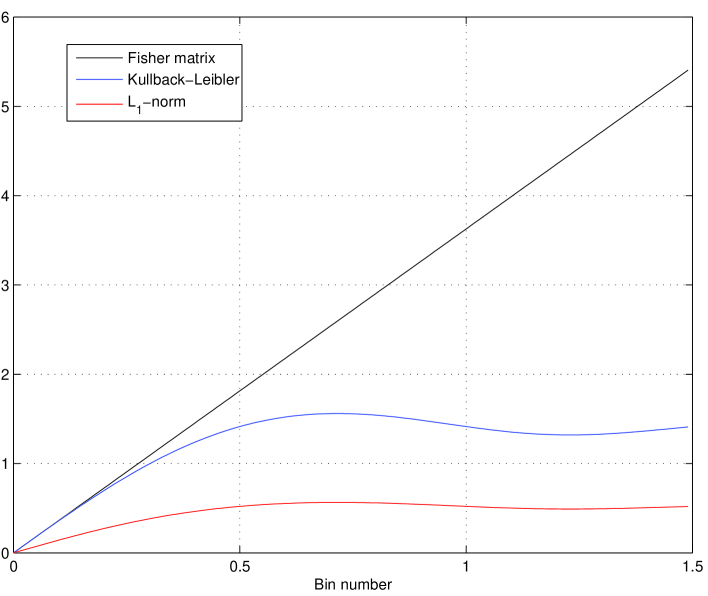
Figure 1: Comparison of the $L_{1}$-norm distance, the Kullback-Liebler divergence, and the line element defined by the Fisher matrix for the case of two monochromatic signals with the same amplitudes and phases but different frequencies as functions of frequency difference expressed in Fourier bins.

As we shall see in the Section 7.2 below we can apply the distance measures to construction of a grid of templates by considering $s_{1}$ as a signal and $s_{2}$ as a template. Taylor expansion may be a good approximation for a very fine grid. However for computationally intensive searches like a search for periodic sources [12, 13] where one needs to choose a loose grid the Taylor expansion of KL-divergence up to second order terms is not accurate.

7 Applications

Using the example of the monochromatic signal let us consider several applications of the distance $d_{L}$ to problem of detection of signal in noise and estimation of parameters.

7.1 Signal resolution

The distance $d_{L}(s_{1},s_{2})$ determines how well we can resolve two signals $s_{1}$ and $s_{2}$. The larger the distance the better the signal resolution. It is useful to have a reduced form of the distance that depends only on the frequencies $\omega_{1}$ and $\omega_{2}$. We can achieve a reduction of the phase parameter by considering the worst case i.e. the minimum of the distance $d_{L}$ given by Eqs.  (58) and (60) over the phase difference $\Delta\phi$. One easily finds an analytic formula for this minimum.

$$d_{Lmin}=erf\left[\frac{1}{2\sqrt{2}}\sqrt{\rho_{1}^{2}+\rho_{2}^{2}-2\rho_{1}\rho_{2}\sqrt{\frac{2(1-\cos(\Delta\omega T))}{(\Delta\omega T)^{2}}}}\right].$$ (64)

There is no nontrivial minimum with respect to amplitudes (the minimum of $d_{Lmin}$ with respect to amplitudes $A_{1}$ and $A_{2}$ is zero). In Figure 2 we plot the distance $d_{L}$ given by Eq. (64) as a function of the difference in angular frequencies $\Delta\omega$ expressed in Fourier bins. We assume that signal-to-noise ratios of the signals $s_{1}$ and $s_{2}$ are equal and equal to 3.

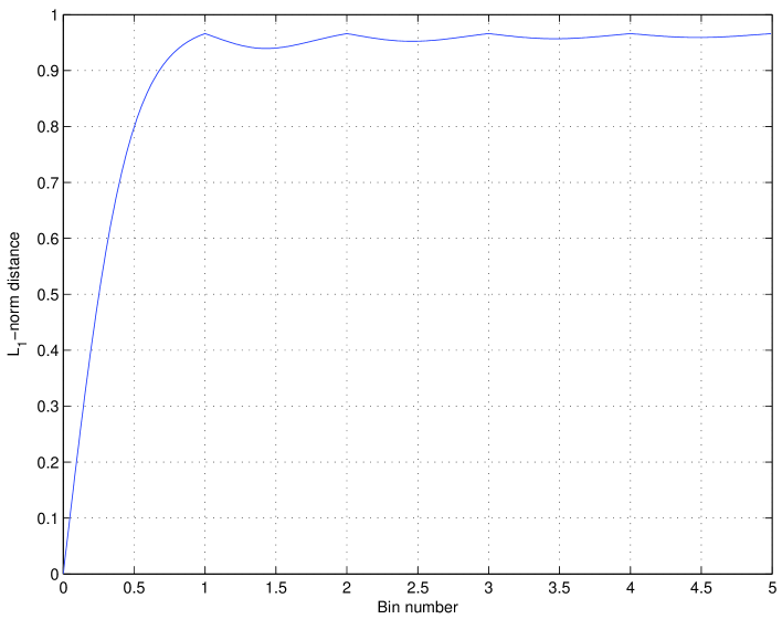
Figure 2: $L_{1}$-norm distance between Gaussian probability density functions for two monochromatic signals as a function of their frequency difference. We assume that the signal-to-noise ratios of both signals are equal to 3.

We see that the distance increases as the difference between the frequencies increases. We also see that there is a substantial increase in the distance when the difference in frequencies between the two signal becomes one bin. This characteristic increase over one bin is independent of the signal-to-noise ratios of the signals. This justifies a folk theorem that two monochromatic signals can be resolved when their frequencies differ by one bin. In Figure 3 we have plotted the distance as a function of signal-to-noise ratios of the two signals for a fixed difference between the frequencies of the signals equal to one bin.

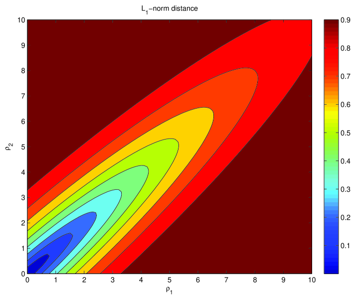
Figure 3: $L_{1}$-norm distance as a function of signal-to-noise ratios $\rho_{1}$ and $\rho_{2}$ of two signals for a fixed difference between the frequencies of the signal equal to one bin.

We see that the distance $d_{L}$ increases as the signal-to-noise ratio increases and also as the difference between the signal-to-noise ratios of the two signals increases. We see that we can achieve an arbitrary large distance and consequently arbitrary large resolvability of the signal if its signal-to-noise ratio is sufficiently large.

7.2 Grid of templates

We can use the distance $d_{L}$ in construction of the grid of templates. We construct the grid of templates in such a way that the maximum distance between a signal and a filter is less than a certain specified value. Let us first calculate the distance $d_{L}(s,s_{F})$ where $s$ is the signal with parameters $A_{o},\phi_{o},\omega_{o}$ and $s_{F}$ is the template. The template $s_{F}$ is just a monochromatic signal with some test parameters $A_{F},\phi_{F},\omega_{F}$. From Section 2 we know that the optimal statistic ${\mathcal{F}}$ is invariant with respect to transformation of the amplitude and the phase of the filter and we can set the amplitude of the filter $A_{F}$ so that its signal-to-noise ratio is equal to 1 and we can choose the phase of the filter $\phi_{F}$ to be equal to $0$. With these simplifications the distance $d_{L}$ is given by

$$d_{L}=erf\left\{\frac{1}{2\sqrt{2}}\sqrt{\rho^{2}+1-2\rho[<\cos(\Delta\omega t)>\cos(\phi_{o})-<\sin(\Delta\omega t)>\sin(\phi_{o})}]\right\}.$$ (65)

Since the ${\mathcal{F}}$-statistic depends only on the frequency we only need the grid in the frequency space and consequently we need to obtain a reduced distance that depends only on the frequencies of the signal and filter. Again like in the case of signal resolution it is natural to consider the worst case scenario. In this case it corresponds to maximum of the distance $d_{L}$ with respect to phase of the signal $\phi_{o}$. We easily get

$$d_{Lmax}=erf\left[\frac{1}{2\sqrt{2}}\sqrt{\rho^{2}+1+2\rho\sqrt{\frac{2(1-\cos(\Delta\omega T))}{(\Delta\omega T)^{2}}}}\right].$$ (66)

The function $d_{Lmax}$ for signal-to-noise ratio $\rho>0$ is a monotonically increasing function of $\rho$. We choose the grid using the distance $d_{L}$ to determine the covering radius of the grid. To calculate the covering radius we can set the signal-to-noise ratio $\rho$ in Eq. (66) equal to the threshold value of $\rho$ used in the search. In Figure 4 we plot the distance $d_{Lmax}$ as a function of the frequency difference $\Delta\omega$ between the signal and the filter for signal-to-noise equal to 8.

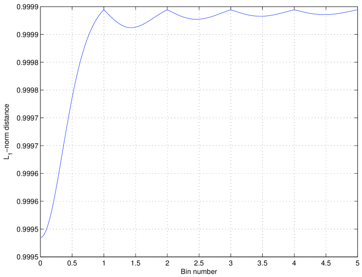
Figure 4: $L_{1}$-norm distance maximized over phase as a function of frequency spacing for a monochromatic signal. The signal-to-noise ratio is set to 8.

7.3 Search templates

Very often we do not have the exact model of the signal that we are searching for. Let us suppose that the signal that we expect to detect in noise is linearly modulated in frequency and has the following form

$$s=A_{o}\cos(\omega_{o}t+\omega_{1}t^{2}+\phi_{o}).$$ (67)

Let us also suppose that we know that $\omega_{1}$ is small and we can expect to detect the signal (67) with a monochromatic signal template that has no frequency modulation. The distance $d_{L}$ is given by

$$d_{L}=erf\left\{\frac{1}{2\sqrt{2}}\sqrt{\rho^{2}+1-2\rho[S\cos(\Delta\phi)-C\sin(\Delta\phi)}]\right\},$$ (68)

where

$$S=<\sin(\Delta\omega t+\omega_{1}t^{2})>,$$ (69)

$$C=<\cos(\Delta\omega t+\omega_{1}t^{2})>.$$ (70)

To determine the quality of the search template we need to find the minimum of the distance with respect to parameters of the filter. The minimum of $d_{L}$ with respect to phase $\phi_{F}$ of the filter can easily be obtained and is given by

$$d_{Lmin}=erf[\frac{1}{2\sqrt{2}}\sqrt{\rho^{2}+\rho^{2}_{F}-2\rho\rho_{F}\sqrt{S^{2}+C^{2}}}].$$ (72)

The minimum value $d_{Lmin}$ is independent of the phase of $\phi_{o}$ of the signal. The minimum is a monotonic function of $\rho$. Consequently to find the minimum of $d_{L}$ with respect to the frequency parameter $\omega_{F}$ of the filter is equivalent to find the maximum of the function

$$FF=\sqrt{S^{2}+C^{2}}$$ (73)

with respect to $\omega_{F}$. In Figure 5 we have plotted the distance (72) as a function of the frequency difference between the template and the signal expressed in frequency bins. For the case of perfectly matched filter ($\omega_{1}=0$) the distance would have a minimum equal to $0$ for $\Delta\omega=0$. For non-zero value of $\omega_{1}$ the minimum distance is larger than zero and it occurs for a certain frequency of the filter biased with respect to true frequency of the signal.

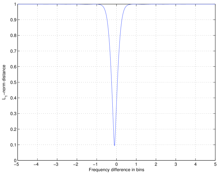
Figure 5: The $L_{1}$-norm distance between the frequency modulated signal and a monochromatic signal filter for frequency modulation parameter $\omega_{1}=2\pi/10/T^{2}$.

8 Conclusion

We have introduced the $L_{1}$-norm distance $d_{L}(p_{1},p_{2})$ between probability density functions $p_{1}$ and $p_{2}$. The $L_{1}$-norm provides a notion of distance between probability distributions endowed with a clear probabilistic interpretation, as discussed in Section 3. The $L_{1}$-norm distance can be a useful tool in gravitational wave data analysis for studying the problem of signal resolution, template placements, and design of search templates. In a future paper we shall study these problems for realistic gravitational wave signals from supernovae, inspiralling binaries, rotating neutron stars and white dwarf binaries.

References

References

- [1] Cutler, C. et al, Phys. Rev. Lett. 70, 2984–2987 (1993).
- [2] Brady, P.R. and Creighton, T. and Cutler, C. and Schutz, B.F., Phys. Rev. D 57, 2101–2116 (1998).
- [3] Jaranowski, P. and Królak, A., Gravitational Wave Data Analysis: Formalism and Applications, Living Rev. Rel., lrr-2005-3,(2005), http://relativity.livingreviews.org/Articles/lrr-2005-3/
- [4] Owen, B., Search templates for gravitational waves from inspiraling binaries: Choice of template spacing, Phys. Rev. D53, 6749–6761, (1996).
- [5] Conway, J.H. and Slone, N.J.A., Sphere packings, latices and groups, Springer (New York), (1999).
- [6] Helström, C.W, Statistical Theory of Signal Detection, Springer (New York), (1995).
- [7] Davis, M.H.A., A Review of Statistical Theory of Signal Detection, in Gravitational Wave Data Analysis, 73–94, Kluwer (Dordrecht), (1989).
- [8] Neyman, J. and Pearson, E., On the problem of the most efficient tests of statistical hypothesis, Phil. Trans. Roy. Soc. Ser. A231, 289–337, (1933).
- [9] Cramér, H., Mathematical Methods of Statistics, Princeton, (1946).
- [10] Kullback, S. and Leibler, R. A., On information and sufficiency, Ann. of Math. Stat. 22, 79–86 (1951).
- [11] T. A. Apostolatos, Phys. Rev. D 52, 605 (1995).
- [12] Astone, P., Borkowski, K.M., Jaranowski, P., and Królak, A., Data Analysis of gravitational-wave signals from spinning neutron stars. IV. An all-sky search, Phys. Rev. D 65, 042003, (2002).
- [13] LIGO Scientific Collaboration, Coherent searches for periodic gravitational waves from unknown isolated sources and Scorpius X-1: results from the second LIGO science run, arXiv:gr-qc/0605028.