Investigation of Lattice QCD with Wilson fermions with Gaussian Smearing

Abstract

We present a detailed study of pion and rho mass, decay constants and quark mass in Lattice QCD with two flavors of dynamical quarks. We use Wilson gauge and fermion action at $\beta=5.6$ on $16^{3}\times 32$ lattice at eight values of the Wilson hopping parameter in the range 0.156 - 0.158. We perform a detailed investigation of the effect of gaussian smearing on both source and sink. We determine the optimum smearing parameter for various correlators for each value of the Wilson hopping parameter. The effects of smearing on observables are compared with those measured using local operators. We also investigate systematic effects in the extraction of masses and decay constants using different types of correlation functions for pion observables. We make interesting observations regarding chiral extrapolations and finite volume effects of different operators.

I Introduction

Among the various formulations of Lattice QCD, the Wilson formulation wilson (both gauge and fermion action) proposed long ago is still attractive due to many reasons, first and foremost being the conceptual simplicity. The Wilson formulation preserves discrete symmetries of the continuum formulation which simplifies the construction of lattice operators that correspond to the observables in the continuum theory. However, because of the explicit violation of chiral symmetry by a dimension five kinetic operator, Wilson formulation has been difficult to simulate at light quark masses. Absence of chiral symmetry implies that the $``$physical” quark mass is no longer proportional to the bare quark mass and the quark mass renormalization is no longer only multiplicative. Lack of chiral symmetry means that the Wilson-Dirac operator which is a sum of anti-Hermitian and Hermitian terms is not protected from arbitrarily small eigenvalues and may lead to zero or near zero modes for individual configurations. This is the infamous problem of $``$exceptional configurations”. This leads to convergence difficulties for fermion matrix inversion which is an integral part of both the generation of gauge field configurations with dynamical fermions and for the computation of hadronic correlation functions via quark propagators. This poses difficulties for lattice simulations with Wilson fermions in the chiral region. The situation has improved recently partly due to the finding deldebbiojhep that the numerical simulations are safe from accidental zero modes for large volumes.

Very generally, the major challenges of probing the chiral regime of lattice QCD are: a) to be able to achieve small lattice spacing $a$ to reduce scaling violations, b) to have small current quark masses to have reliable chiral extrapolations, and c) to have large enough physical volume of the lattice to avoid finite size effects. In addition, lattice QCD investigations suffer from uncertainties regarding the determination of the lattice scale and inaccuracies in derived quantities of interest, e.g., hadronic masses, decay constants etc. Many of the above issues are connected.

We have planned on a detailed lattice QCD investigation with Wilson and Wilson-type fermions. In this work we have taken the first step towards addressing the above issues systematically. We study smearing of mesonic operators with standard (unimproved) Wilson gauge and fermion actions with 2 fully dynamical light quark flavors on $16^{3}32$ lattice, $\beta=6/g^{2}=5.6$ at 8 values of bare quark masses (corresponding to fermionic hopping parameter $\kappa=0.156,~{}0.1565,~{}0.15675,~{}0.157,~{}0.15725,~{}0.1575,~{}0.15775,~{}0.158$). The lattice scale reached is respectable and $a\sim 0.08$ fm ($a^{-1}\sim 2.45GeV$). It is important to have a small enough $a$ to hopefully have small scaling violations and then evaluate the low lying spectrum of QCD accurately and to study cleanly chiral extrapolations in finite volumes. We plan on having larger volumes and larger $\beta$ in the near future with more sophisticated algorithmic developments discussed in deldebbiojhep ; deldebbio1 ; deldebbio2 ; japo . In the present work our emphasis is to have fully dynamical simulations at an extensive set of $\kappa$ values and study accurate determinations of the masses and decay constants in as many ways as possible.

In a separate paper qcd_paper1 , we investigate quite elaborately the determination of the lattice scale from the potential between a heavy quark-antiquark pair. We study the observed change of $r_{0}/a$ with bare quark masses where $r_{0}$ is the Sommer parameter sommer and resulting uncertainties of scale determinations and also discuss its relation with the chiral extrapolation of observables. For a recent review on various approaches to scale determination and associated issues, see Ref. mcneile .

The masses in Lattice Gauge Theory are calculated from the asymptotic behaviour of Euclidean time correlation functions. The contribution from the lowest mass state dominates for large time. Thus, to get a clean signal one has to make the length in the time direction as large as possible. But this is computationally expensive. Furthermore, as the time increases, the signal to noise ratio gets smaller which results in larger statistical errors. To reduce the statistical error, we need to increase the number of measurements (configurations). This is also computationally expensive. Hence there is a practical need for techniques that allow one to reliably extract observables still working on moderately sized time direction and not too large number of configurations.

For the measurement to be in the scaling region, one needs to go to smaller and smaller lattice spacings. But as the lattice spacing decreases, the physical hadron state will extend over more and more lattice spacings. Thus a state created by a local operator from the vacuum will have less and less overlap with the physical state as the lattice spacing decreases. To improve the measurements, it is useful to use operators that have larger overlaps with the physical state (which is extended). This will naturally lessen the contamination from higher mass states to the correlation functions. Smearing of operators is one way to achieve this goal, thereby reducing the necessity to have both large time direction and large number of configurations.

One of the earliest references discussing the need for smearing is Ref. parisi . Earliest suggestions for smearing involved Dirac delta functions on source time slices, the so-called wall source. See for example, Ref. billoire . So far, in the literature, smearing has been implemented in two different methods, namely, the gauge invariant method and the gauge fixed method. Gauge fixed wall source smearing, exponential smearing and gaussian smearing belong to the second method. Gauge fixed wall source smearing is used in some work of JLQCD aoki-stagg and MILC milc3 Collaborations. Exponential smearing is used in some works of CP-PACS alikhan and JLQCD aoki Collaborations. Gaussian smearing was first considered by DeGrand and Loft delo1 , and used, e.g., in Ref. bitar ; hauswirth ) (with dynamical quarks) and in Ref. ibm ; milcw ; degrand1 ; degrand2 (with quenched quarks) in different contexts. A clear discussion of smearing (in the context of gaussian smearing) and the associated Fourier Transformation $``$trick” is provided in the Ph. D. thesis of Hauswirth hauswirth .

To the best of our knowledge, a systematic study of the effects of gaussian smearing on source or/and sink operators does not seem to be available in the literature. In this work we carry out a detailed investigation of the effect of gaussian smearing on the source or/and sink meson operators.

At a particular value of the smearing size, a variety of correlation functions are to be measured to extract meson observables. For example, for the pion, PP, AA, AP and PA correlators can be used since both P and A carry quantum numbers of pion. (Here P and A denotes psudoscalar and the fourth component of the axial vector densities respectively.) Mass gaps and amplitudes (coefficients) are extracted for the smearing radius $s_{0}$ ranging from 1 to 8 in steps of 1. We also carry out extensive calculations with local operators. This helps us to quantify the systematic effects in the determination of masses and decay constants.

We present results for the pion mass, the rho mass, their decay constants and the quark mass (all in units of the lattice constant $a$). Although this paper is not intended to deal with the issues of chiral extrapolation of pseudoscalar observables, especially at our relatively large masses with $16^{3}32$ lattices, we make interesting observations regarding consistency with $\chi PT$. In this connection, we also comment on finite volume effects on part of our data at the largest $\kappa$. We have also noticed varying finite size effects on different pion operators.

This paper is organized as follows. In Sec. II we present the lattice action and the details of the simulation. Expressions for the local observables that we calculate are given in Sec. III. Sec. IV introduces the gaussian smearing and different fitting ansaetze for the correlator data analysis are given in Sec. V. Details of the implementation of smearing are in Sec. VI. Results for pion and rho observables are presented in Secs. VII and VIII respectively. Finally, the summary and the conclusions are presented in Sec. IX. For the sake of completeness and clarity, the Fourier transform method employed in the case of sink smearing is presented in Appendix A.

II Simulation

II.1 Action

We have performed simulations with the standard Wilson action $S~{}=~{}S_{F}~{}+~{}S_{G}$ where the standard Wilson gauge action is given by

$$S_{G}=~{}\beta~{}\sum\left[1-\frac{1}{3}~{}{\rm Re}~{}{\rm Trace}~{}U_{P}\right],$$

with $\beta=\frac{6}{g^{2}}$ ($g$ is the $SU(3)$ gauge coupling), the elementary plaquette $U_{P}$ being the product of $SU(3)$ link fields $U$ around the elementary square of the hypercubic lattice and the standard Wilson fermion action is given by

$$S_{F}[\psi,{\overline{\psi}},U]=\sum_{x,y}{\overline{\psi}}_{x}M_{xy}\psi_{y}~{}~{}{\rm with}~{}~{}$$ (1)

$$M_{xy}=\delta_{xy}-\kappa\left[\left(r-\gamma_{\mu}\right)U_{x,\mu}~{}\delta_{x+\mu,y}+\left(r+\gamma_{\mu}\right)U^{\dagger}_{x-\mu,\mu}~{}\delta_{x-\mu,y}\right]~{}.$$ (2)

We have suppressed spin, color and flavor indices in the quark fields $\psi$ and $\overline{\psi}$ and the fermion matrix $M$. As usual, we have taken the Wilson parameter $r=1$. We consider two degenerate light quark flavors, i.e., $N_{F}=2$.

II.2 Details of Simulation

The gauge coupling $\beta=5.6$ and the lattice volume is $16^{3}\times 32$. The hopping parameter $\kappa$=0.156, 0.1565, 0.15675, 0.157, 0.15725, 0.1575, 0.15775 and 0.158. At each $\kappa$ we have generated 5000 equilibrated configurations with the standard HMC algorithm (with even-odd pre-conditioned Conjugate Gradient for inversion of $M^{\dagger}M$) and performed the mesonic correlator measurements separated by 25 trajectories. The time step size is chosen to be 0.01 and the number of steps per trajectory is 100. The stopping criterion for the residue of the conjugate gradient $\sqrt{\mid R\mid^{2}/\mid\chi\mid^{2}}\leq 10^{-5}$ is used for all $\kappa$ values except 0.158 (for which it is $10^{-6}$) where $R=M^{\dagger}M\zeta-\chi$ ($\chi$ and $\zeta$ are respectively the source and the iterative solution). Stabilized BICG algorithm is used for the inversion of $M$ needed for the mesonic correlators, the stopping criterion of the residue for very accurate inversion in this case is chosen as $10^{-9}$ and $10^{-10}$.

The parameters are chosen such that the acceptance rate is above 75 % for $\kappa$ less than 0.157 and around 65 % for $\kappa$ above and including 0.157.

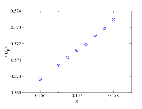
Figure 1: Average value of the Plaquette versus $\kappa$.

Fig. 1 shows that the expectation value of the average plaquette has a smooth behavior in dependence of $\kappa$.

II.3 Auto correlation

For any particular observable ${\mathcal{O}}$, autocorrelations among the generated configurations are generally determined by the integrated autocorrelation time $\tau_{\rm int}^{\mathcal{O}}$ for that observable. For this purpose, at first, one needs to calculate the unnormalized autocorrelation function of the observable ${\mathcal{O}}$ measured on a sequence of $N$ equilibrated configurations as

$$C^{\mathcal{O}}\left(t\right)=\frac{1}{N-t}\sum_{r=1}^{N-t}\left({\mathcal{O}}_{r}-\langle{\mathcal{O}}\rangle_{L}\right)\left({\mathcal{O}}_{r+t}-\langle{\mathcal{O}}\rangle_{R}\right)$$ (3)

where, instead of the usual single mean-value estimator, we have used the “left” and “right” mean-value estimators

$$\langle{\mathcal{O}}\rangle_{L}=\frac{1}{N-t}\sum_{s=1}^{N-t}{\mathcal{O}}_{s},~{}~{}~{}~{}\langle{\mathcal{O}}\rangle_{R}=\frac{1}{N-t}\sum_{s=1}^{N-t}{\mathcal{O}}_{s+t}$$ (4)

for a faster convergence as claimed in orthprd .

Following the “windowing” method as recommended by Ref. sokal , we have calculated the integrated autocorrelation time as

$$\tau_{\rm int}^{\mathcal{O}}=\frac{1}{2}+\sum_{t=1}^{t_{\rm cut}}\rho^{\mathcal{O}}\left(t\right)$$ (5)

where

$$\rho^{\mathcal{O}}\left(t\right)=C^{\mathcal{O}}\left(t\right)/C^{\mathcal{O}}\left(0\right)$$ (6)

is the normalized autocorrelation function.

The factor of $\frac{1}{2}$ in the Eq. (5) is purely a matter of convention and is chosen such as to guarantee that for $N\rightarrow\infty$, the normalized autocorrelation function behaves as ${\rm exp}\left(-t/\tau_{\rm int}^{\mathcal{O}}\right)$ with $\tau_{\rm int}^{\mathcal{O}}\gg 1$.

If plotted against the variable cutoff $t_{\rm cut}$, the resulting values of $\tau_{\rm int}^{\mathcal{O}}$ ideally show a plateau but instead a peak or monotonous rise is also observed sometimes. Following the suggestions of sokal , we have drawn two straight lines $t_{\rm cut}/4$ and $t_{\rm cut}/10$ respectively and have chosen $\tau_{\rm int}^{\mathcal{O}}$ inspecting only the segment of the curve lying within its intersections with the two straight lines. This ensures a balance between the noise and the bias in the estimation of the autocorrelation time.

We have measured the integrated autocorrelation times for the average values of the Plaquette and the number of Conjugate Gradient iterations, called ${\rm Niter}$, during HMC trajectories for the generated configurations for each value of $\kappa$. The errors are calculated by the single omission jackknife method. Our results are presented in the Table 1. Despite fluctuations, $\tau_{\rm int}$ in general increases with larger $\kappa$ especially as $\kappa$ approaches $\kappa_{c}$.

A typical example of the expected plateau of $\tau_{\rm int}$ as a function of $t_{\rm cut}$ for both the average Niter and Plaquette at $\kappa=0.157$ is shown in Fig. 2.

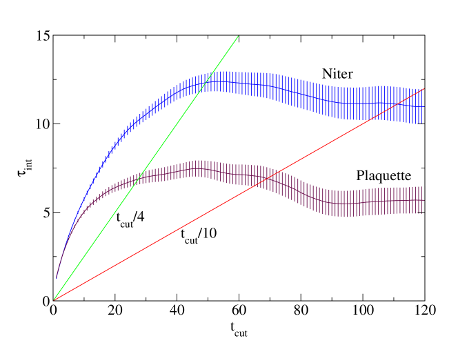
Figure 2: Integrated autocorrelation time $\tau_{\rm int}$ for both average Niter and Plaquette at $\kappa$=0.157.

$\kappa$	Niter	Plaquette
0.156	13(1)	5.4(3)
0.1565	14(1)	11(1)
0.15675	19(1)	8(1)
0.157	12(1)	7(1)
0.15725	26(1)	11(1)
0.1575	21(1)	8(1)
0.15775	14(1)	9(1)
0.158	27(2)	10(1)

Table 1: Integrated Autocorrelation time $\tau_{int}$ for Average Niter and Plaquatte as a function of $\kappa$.

III Observables with local operators

We measure the charged pion and the rho propagators to extract masses, decay constants and the quark mass at each $\kappa$.

For pion, we measure the following zero-spatial-momentun correlation functions on a $L^{3}T$ lattice as functions of the Euclidean time $t$:

$$C_{1}(t)~{}~{}=~{}~{}\langle 0\mid{\cal O}^{\dagger}(t){\cal O}(0)\mid 0\rangle~{}~{}\stackrel{{\scriptstyle t\rightarrow\infty}}{{\longrightarrow}}~{}~{}C^{\cal OO}\Big{[}e^{-m_{\pi}t}~{}+~{}e^{-m_{\pi}(T-t)}\Big{]}$$

$$C_{2}(t)~{}~{}=~{}~{}\langle 0\mid{\cal O}_{1}^{\dagger}(t){\cal O}_{2}(0)\mid 0\rangle~{}~{}\stackrel{{\scriptstyle t\rightarrow\infty}}{{\longrightarrow}}~{}~{}C^{{\cal O}_{1}{\cal O}_{2}}\Big{[}e^{-m_{\pi}t}~{}-~{}e^{-m_{\pi}(T-t)}\Big{]}$$

The coefficients are given by,

$$C^{\cal OO}=\frac{1}{2m_{\pi}}\mid\langle 0\mid{\cal O}(0)\mid\pi\rangle\mid^{2}$$

$$C^{{\cal O}_{1}{\cal O}_{2}}~{}=~{}\frac{1}{2m_{\pi}}\langle 0\mid{\cal O}_{1}^{\dagger}(0)\mid\pi\rangle\langle\pi\mid{\cal O}_{2}(0)\mid 0\rangle~{}.$$

${\cal OO}\equiv PP$ or $AA$ and ${{\cal O}_{1}{\cal O}_{2}}=AP$ or $PA$ where $P={\overline{q}}_{i}\gamma_{5}q_{j}~{}~{}~{}{\rm and}~{}~{}A_{4}={\overline{q}}_{i}\gamma_{4}\gamma_{5}q_{j}~{}$ denote the pseudoscalar density and fourth component of the axial vector current ($i$ and $j$ stand for flavor indices for the $u$ and $d$ quarks, for the charged pion $i\neq j$).

For clarity and to set up our notation, in the following we discuss all the possible ways of determining the decay constants and the PCAC quark masses.

III.1 Pion Decay Constant

The pion decay constant $F_{\pi}$ and the quark mass $m_{q}$ from PCAC or the axial Ward identity are respectively defined, in the continuum, via

$$\langle 0\mid A_{\mu}(0)\mid\pi(p)\rangle = \sqrt{2}F_{\pi}p_{\mu},$$ (7)

$$\partial_{\mu}A_{\mu}(x) = 2m_{q}P(x).$$ (8)

Since we measure the PP, PA, AP and AA correlators, we have a variety of ways to compute the pion decay constant and the PCAC quark mass.

Method I: From the AA correlator

$$C(t)~{} = ~{}\langle 0\mid A_{4}^{\dagger}(t)A_{4}(0)\mid 0\rangle~{}$$ (9)

$$\stackrel{{\scriptstyle t\rightarrow\infty}}{{\longrightarrow}} C^{AA}\Big{[}e^{-m_{\pi}t}~{}+~{}e^{-m_{\pi}(T-t)}\Big{]}$$ (10)

where $C^{AA}=\frac{1}{2m_{\pi}}\mid\langle 0\mid A_{4}(0)\mid\pi\rangle\mid^{2}$, and the pion decay constant as defined in Eq. (7) follows

$$F_{\pi}^{AA}~{}=~{}2\kappa~{}\sqrt{\frac{C^{AA}}{m_{\pi}}}~{}.$$ (11)

The factor $2\kappa$ above accounts for the difference in normalization between the continuum and the Wilson lattice fermion actions.

It is obvious that the $m_{\pi}$ that appears in Eq. (11) is numerically obtained from the $AA$ correlator. If numerically $m_{\pi}$ is obtained from another correlator, say the PP, then one needs to put that mass in the fit Ansatz for the AA correlator to obtain the coefficient $C^{AA}$.

Method II: From the PP and the AP propagators

$$C^{PP} = \frac{1}{2m_{\pi}}\mid\langle 0\mid P(0)\mid\pi\rangle\mid^{2}$$ (12)

$$C^{AP} = \frac{1}{2m_{\pi}}\langle 0\mid A_{4}(0)\mid\pi\rangle\langle\pi\mid P^{\dagger}(0)\mid 0\rangle$$ (13)

which lead to

$$F_{\pi}^{AP}~{}=~{}\frac{2\kappa~{}C^{AP}}{\sqrt{m_{\pi}C^{PP}}}.$$ (14)

Similarly using the PP and the PA propagators

$$F_{\pi}^{PA}~{}=~{}\frac{2\kappa~{}C^{PA}}{\sqrt{m_{\pi}C^{PP}}}.$$ (15)

For numerical evaluation of $F_{\pi}$ using Eqs. (14) and (15), the values of $m_{\pi}$ computed from PP, AP and PA correlators have to be the same, which is hard to achieve numerically. Hence it is advisable to use the best determined mass from one particular correlator and then use that value in the other correlators to determine all the coefficients $C$. The same applies also to the determination of the different PCAC quark masses discussed below.

III.2 PCAC Quark Mass

Method I: From $\partial_{\mu}A_{\mu}(x)=2m_{q}P(x),$ summing over spatial coordinates,

$$\sum_{\bf x}\partial_{\mu}A_{\mu}(x)=2m_{q}\sum_{\bf x}P(x)\Longrightarrow\partial_{4}A_{4}(t)=2m_{q}P(t).$$ (16)

Taking the matrix element between the vaccum and physical pion states we have

$$m_{\pi}\langle 0\mid A_{4}(0)\mid\pi\rangle=2m_{q}\langle 0\mid P(0)\mid\pi\rangle$$ (17)

which leads to

$$m_{q}^{AA}~{}=~{}\frac{m_{\pi}}{2}~{}\sqrt{\frac{C^{AA}}{C^{PP}}}~{}.$$ (18)

Method II: Using PCAC

$$\partial_{\mu}\langle 0\mid A_{\mu}(x)P^{\dagger}(0)\mid 0\rangle=2m_{q}\langle 0\mid P(x)P^{\dagger}(0)\mid 0\rangle$$ (19)

Summing over spatial coordinates

$$\sum_{\bf x}\partial_{\mu}\langle 0\mid A_{\mu}(x)P^{\dagger}(0)\mid 0\rangle=2m_{q}\sum_{\bf x}\langle 0\mid P(x)P^{\dagger}(0)\mid 0\rangle$$ (20)

At large $t$,

$$\partial_{4}C^{AP}\Big{[}e^{-m_{\pi}t}-e^{-m_{\pi}(T-t)}\Big{]}=2m_{q}C^{PP}\Big{[}e^{-m_{\pi}t}+e^{-m_{\pi}(T-t)}\Big{]}$$ (21)

which leads to

$$m_{q}^{AP}=\frac{m_{\pi}}{2}~{}\frac{C^{AP}}{C^{PP}},~{}~{}~{}~{}~{}~{}~{}~{}~{}~{}~{}~{}m_{q}^{PA}=\frac{m_{\pi}}{2}~{}\frac{C^{PA}}{C^{PP}}$$ (22)

III.3 Rho Mass and Decay Constant

There are two different definitions of $\rho$ deacy constant used in the literature.

$$\langle 0\mid V_{\mu}(0)\mid\rho\rangle~{}=~{}\epsilon_{\mu}~{}\frac{m_{\rho}^{2}}{f_{\rho}}$$ (23)

where $f_{\rho}$ is dimensionless and

$$\langle 0\mid V_{\mu}(0)\mid\rho\rangle~{}=~{}\epsilon_{\mu}\sqrt{2}F_{\rho}m_{\rho}$$ (24)

with $V_{\mu}(0)={\overline{q}}(0)\gamma_{\mu}q(0)$ and $\epsilon_{\mu}$ is the polarization vector of rho.

Here $F_{\rho}$ is dimensionful and $F_{\rho}/m_{\rho}=(f_{\rho})^{-1}$.

Mass and decay constant of rho are calculated from the correlation function

$$C(t)~{} = ~{}\langle 0\mid V_{3}^{\dagger}(t)V_{3}(0)\mid 0\rangle~{}$$ (25)

$$\stackrel{{\scriptstyle t\rightarrow\infty}}{{\longrightarrow}} C^{VV}\Big{[}e^{-m_{\rho}t}~{}+~{}e^{-m_{\rho}(T-t)}\Big{]}$$ (26)

where, $C^{VV}=\frac{1}{2m_{\rho}}\mid\langle 0\mid V_{3}(0)\mid\rho\rangle\mid^{2}$. Thus

$$F_{\rho}/m_{\rho}=1/f_{\rho}~{}=~{}2\kappa~{}\sqrt{\frac{C^{VV}}{m_{\rho}^{3}}}~{}.$$ (27)

We compute the decay constants and the quark masses according to the expressions given above, but to obtain their values in the continuum one needs to multiply with appropriate factors of renormalization constants $Z_{P}$, $Z_{A}$ and $Z_{V}$ associated with lattice pseudoscalar, axial vector and vector densities respectively. Although we have made approximate estimations of $Z_{A}$ and $Z_{V}$ in Sec. VIII, we do not quote numbers in the continuum in this paper.

IV Gaussian Smearing

To increase the overlap with the hadronic ground state, many, if not most, QCD spectrum calculations traditionally use the method of smearing the hadronic interpolating operator, essentially making the hadronic operator spread around their central location in space. In this work, for the pion and the rho operators, we have used the so-called gaussian smearing where one uses a shell model trial wave function with one variational parameter, $\phi(r)\sim\exp\left(-\left(r/s_{0}\right)^{2}\right)$. For details please see Ref. [delo1 ]. $s_{0}$ is the smearing size parameter.

An advantage of the gaussian smearing is that the smearing function, for example for a meson operator, separates into two factors one belonging to the quark and the other to the antiquark. This has certain numerical advantages, especially for sink smearing. However, the smeared operators are no longer gauge-invariant because the quark and the antiquark are spatially separated. We have used Coulomb gauge fixing to obtain non-zero expectation values.

The coefficients $C^{{\cal O}_{1}{\cal O}_{2}}$ for local operators are needed, as described in Sec. III to calculate the decay constants and the PCAC quark masses. One can take a mixed approach where one evaluates the hadron mass from a hadronic propagator which uses smearing at either the source or the sink or at both places, and at the same time calculate the coefficient $C^{{\cal O}_{1}{\cal O}_{2}}$ from the local-local propagator (as pursued in Ref. milc3 ). For this to work, large time-extents are necessary. However, if one wants to calculate the local-local coefficients from the smeared propagators, one needs to calculate the propagators with all combinations of smearing: i) local sink and smeared source ($ls$), ii) smeared sink and local source ($sl$), and (iii) smeared sink and smeared source ($ss$). If they produce the same hadronic mass at large euclidean times, by combining the coeffecients of the three, all calculated with the same smearing parameter $s_{0}$, one is able to calculate the coefficient corresponding to the local-local propagator. This is done as follows.

The large Euclidean time behavior of the correlation function involving local (unsmeared) operators is ${\cal A}$ and ${\cal B}$

$$\langle 0\mid{{\cal A}_{l}^{\rm sink}}^{\dagger}(t)~{}{{\cal B}_{l}^{\rm source}}(0)\mid 0\rangle~{} \stackrel{{\scriptstyle t\rightarrow\infty}}{{\longrightarrow}} C^{\cal AB}_{ll}~{}e^{-m_{H}t}$$

where, $C^{\cal AB}_{ll}~{}=~{}~{}\frac{1}{2m_{H}}\langle 0\mid{{\cal A}_{l}^{\rm sink}}^{\dagger}(0)\mid H\rangle\langle H\mid~{}{{\cal B}_{l}^{\rm source}}(0)\mid 0\rangle~{}$.

Similarly

$$C^{\cal AB}_{ls}~{} = ~{}~{}\frac{1}{2m_{H}}\langle 0\mid{{\cal A}_{l}^{\rm sink}}^{\dagger}(0)\mid H\rangle\langle H\mid~{}{{\cal B}_{s}^{\rm source}}(0)\mid 0\rangle~{}$$

$$C^{\cal AB}_{sl}~{} = ~{}~{}\frac{1}{2m_{H}}\langle 0\mid{{\cal A}_{s}^{\rm sink}}^{\dagger}(0)\mid H\rangle\langle H\mid~{}{{\cal B}_{l}^{\rm source}}(0)\mid 0\rangle~{}$$

$$C^{\cal AB}_{ss}~{} = ~{}~{}\frac{1}{2m_{H}}\langle 0\mid{{\cal A}_{s}^{\rm sink}}^{\dagger}(0)\mid H\rangle\langle H\mid~{}{{\cal B}_{s}^{\rm source}}(0)\mid 0\rangle~{}.$$

Assuming the lowest mass obtained at large Euclidean time to be the same for each of the $ls$, $sl$ and $ss$ correlators, it follows that

$$C_{ll}=C_{ls}C_{sl}/C_{ss}~{}.$$ (28)

V Analysis of Meson Correlation Functions

For our initial investigations we performed four types of fits using exponential functions for the correlation functions of the pion and the rho. For example, for the pion propagator, the fit ansaetze involving two, three, four and five parameters are as follows.

$$C_{I}(t) = C_{1}^{{\cal O}_{1}{\cal O}_{2}}\Big{[}e^{-m_{\pi}t}~{}\pm~{}e^{-m_{\pi}(T-t)}\Big{]}~{},$$

$$C_{II}(t) = C_{1}^{{\cal O}_{1}{\cal O}_{2}}\Big{[}e^{-m_{\pi}t}~{}\pm~{}e^{-m_{\pi}(T-t)}\Big{]}~{}+~{}C_{2}^{{\cal O}_{1}{\cal O}_{2}}\Big{[}e^{-3m_{\pi}t}~{}\pm~{}e^{-3m_{\pi}(T-t)}\Big{]}~{},$$

$$C_{III}(t) = C_{1}^{{\cal O}_{1}{\cal O}_{2}}\Big{[}e^{-m_{\pi}t}~{}\pm~{}e^{-m_{\pi}(T-t)}\Big{]}~{}+~{}C_{2}^{{\cal O}_{1}{\cal O}_{2}}\Big{[}e^{-m_{2}t}~{}\pm~{}e^{-m_{2}(T-t)}\Big{]}~{},$$

$$C_{IV}(t) = C_{1}^{{\cal O}_{1}{\cal O}_{2}}\Big{[}e^{-m_{\pi}t}~{}\pm~{}e^{-m_{\pi}(T-t)}\Big{]}~{}+~{}C_{2}^{{\cal O}_{1}{\cal O}_{2}}\Big{[}e^{-3m_{\pi}t}~{}\pm~{}e^{-3m_{\pi}(T-t)}\Big{]}$$ (29)

$$+ C_{3}^{{\cal O}_{1}{\cal O}_{2}}\Big{[}e^{-m_{3}t}~{}\pm~{}e^{-m_{3}(T-t)}\Big{]}~{}.$$

In the presence of sea quarks, pair creation from vacuum becomes possible and the creation of two quark-antiquark pairs results in two extra pseudoscalar mesons. Thus in the presence of sea quarks, the next higher state can be expected to be a three pion state deldebbio1 . The second and the fourth fit ansaetze above are motivated by this physical picture. The rho propagator can also be treated in the same way, the next higher state there being $2m_{\pi}+m_{\rho}$.

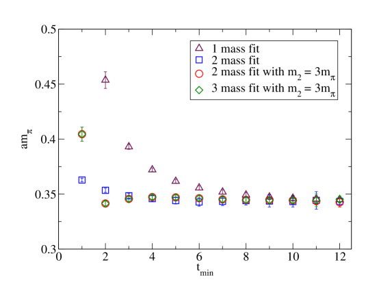
Figure 3: Pion mass obtained from unsmeared PP correlator at $\kappa=0.157$ with four different fits as function of $t_{\rm min}$.

VI Details of the implementation of the gaussian smearing

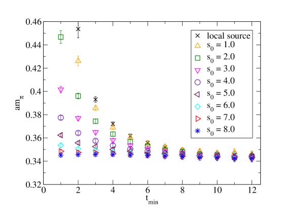
Figure 4: Pion mass from one exponential fit (two parameters) as a function of $s_{0}$.

Figure 5: $C_{AA}$ obtained from constrained and unconstrained fits (data slightly shifted horizontally for clarity on the error bars).

As mentioned earlier, in this paper we present results with two flavors of fully dynamical Wilson (unimproved) quarks (with standard plaquette Wilson gauge action) at $\beta=5.6$ on $16^{3}32$ lattices at an extensive set of the fermion hopping parameter, viz., $\kappa=0.156,~{}0.1565,~{}0.15675,~{}0.157,~{}0.15725,~{}0.1575,~{}0.15775,~{}0.158$.

At this $\beta$ and lattice volume, similar $N_{F}=2$ calculations have been done before at a few $\kappa$ values (for example, see Ref. orthprd ). The previous results help us to have a cross-check and have belief in our numerical procedure. Some data are available at larger volumes with the rest of the parameters staying the same; these give some indication of the finite size effects in our results. However, we like to mention that, to the best of our knowledge, ours are the first calculations at $\beta=5.6$ at $\kappa=0.15675,~{}0.15725~{}~{}{\rm and}~{}~{}0.15775$ for any lattice volume.

At each $\kappa$, we have investigated in detail the PP, AA, AP and PA correlators for the pion and VV correlators for the rho. For each operator, we have used source smearing ($ls$), sink smearing ($sl$) and smearing at both source and sink ($ss$) (see Appendix A for the Fourier transform method for the smeared sources). Then at each $\kappa$, with each operator and each sink-source smearing combination, we have tried eight values for the gaussian smearing size parameter, viz., $s_{0}=1$ to $L/2=8$ (in increment of unity) in order to have optimum smearing (please note that $s_{0}\rightarrow\infty$ produces the so-called wall source).

For comparison, we have also investigated all the above correlators without any smearing, i.e., using local sink and local source (denoted with subscript $ll$).

With or without smearing, our general strategy was to determine the pion mass from the PP and the AA propagators only and not from the asymmetric propagators AP or PA, by reaching a plateau with respect to $t_{\rm min}$ (minimum $t$ used for fitting the formulae 29. In general, the quality of the mass-plateaux for the AP and the PA correlator was not of the same high quality as for the PP and the AA correlators (AA noisier than PP), more true with smearing. As a note of caution, let us also mention that at a few large $\kappa$ values the local-local AA correlators were very noisy, resulting in inaccurate and perhaps unreliable determinations of the all relevant quantities as apparent from fourth data-column of Table 3.

We have used the well-known technique of effective masses by taking ratios of propagators for adjacent time-slices, but only as a rough guide (especially for smeared propagators). We shall not show any effective mass plots in this paper.

In Fig. 3, we show, for the unsmeared ($ll$) PP correlator, the results at $\kappa=0.157$ for $m_{\pi}$ obtained with the four different fit Ansaetze 29, as functions of $t_{\rm min}$ (here and in the subsequent figures, $t_{\rm min}/a$ in the abscissae is indicated as just $t_{\rm min}$. Firstly, we note in Fig. 3 that all the different fits produce good plateaux for appropriately large $t_{\rm min}$ and they all agree with each other. The plot also shows that $3m_{\pi}$ is the next higher state. Unless otherwise specified, all errors in this plot and others to follow are single-omission jackknife statistical errors calculated from 200 jackknife bins of correlator data.

With unsmeared propagators, although it is obvious that longer time-extent would have helped, we have been quite successful in obtaining a reasonable plateau even at lower pion masses with the single exponential ansatz. This was a great advantage because ansaetze with higher number of exponentials are harder to automate for the error calculation because sometimes the order of the masses changes in the fit-results for some bins. We have (almost) always used the single exponential fit for the unsmeared correlators both for the pion and the rho.

Once we determine the pion mass from the PP and the AA correlators, we then respectively use these masses for fitting all the correlators to obtain the coefficients, as discussed in Sec. III and then extract the various decay constants and the quark masses. We have used the same strategy for the smeared propagators too, both for the pion and the rho.

Fig. 4 shows for $\kappa=0.157$ the pion mass determined from single-exponential fits to the PP correlator with local sink and smeared source as a function of $t_{\rm min}$ for all the investigated values of the smearing size parameter $s_{0}=1,2,\ldots,8$. The figure also includes the pion mass obtained by single-exponential fits from the local-local PP correlator for this $\kappa$. The figure shows that $s_{0}=8$ gives the most reliable mass-plateau and we take the mass from the fit with the best confidence level from the plateau at $s_{0}=8$. As discussed below, choice of the optimum $s_{0}$ for a given correlator, PP in this case, has to be the same for all smearing combinations $ls$, $sl$ and $ss$. Hence in this case we made sure that for the other two cases, viz., $sl$ and $ss$, the optimum choice of $s_{0}$ was also 8. Then along with $C^{PP}_{ls}$ obtained from the correlated 2-parameter single-exponential fits to the $ls$ correlator, we also obtained $C^{PP}_{sl}$ and $C^{PP}_{sl}$ at $s_{0}=8$ by making 1-parameter single exponential fit with the value of $m_{\pi}$ put in from the chosen best fit to the $ls$ PP correlator. This process was done for each of 200 jackknife bins so as to get the jackknife statistical errors for all the derived quantities. The errors shown in Fig. 4 are jackknife errors.

Once $m_{\pi}$ is determined from a given correlator (in this $ls$ PP), we can then similarly determine the coefficients for all other correlators (in this case, AA, AP and PA) and for all sink-source smearing combinations. Optimum values of the smearing size $s_{0}$ need not be the same for the other operators. However, it has to be the same for all smearing combinations of the same operator (for applicability of Eq. (28). Once again, for each correlator we looked for the optimum $s_{0}$ by comparing 1-parameter single-exponential fits (with $m_{\pi}$ put in) for all smearing combinations. In Fig. 5 the coefficient $C^{AA}_{ls}$ for the optimum $s_{0}=3$ for the AA correlator is shown as a function of $t_{\rm min}$ again at $\kappa=0.157$ and displays a nice plateau with accurate data points. The figure also compares $C^{AA}_{ls}$ obtained from correlated 2-parameter single-exponential fit (with no $m_{\pi}$ predetermined); coefficients determined in this way show a rough plateau with a lot less accuracy (larger error bars). This is an important point considering that the determination of quark masses and especially the decay constants depend crucially on the accurate determination of the coefficients.

$\kappa$	$s_{0}$
	PP	AA	AP	PA	VV
0.156	3.0	1.0	1.0	1.0	4.0
0.1565	7.0	5.0	4.0	5.0	7.0
0.15675	5.0	3.0	2.0	2.0	7.0
0.157	8.0	3.0	5.0	4.0	8.0
0.15725	6.0	3.0	3.0	3.0	8.0
0.1575	6.0	3.0	3.0	3.0	8.0
0.15775	8.0	4.0	5.0	4.0	8.0
0.158	7.0	7.0	5.0	5.0	8.0

Table 2: Optimum values of the smearing size parameter $s_{0}$ for all correlators investigeted

As mentioned already before while discussing the local-local correlators, the pion masses were always determined from only the PP and the AA correlators also in the case with smeared correlators. In addition, to be consistent across all $\kappa$ values, we have always determined the masses from the local sink - smeared source ($ls$) combination. This is also true for the rho mass where we investigated only the VV correlator.

For the smeared correlators, we first determine the optimum smearing parameter $s_{0}$ for each correlator PP, AA, AP and PA and in general the optimum values are different for different operators (see Table 2). As mentioned already above, for a given operator, the value of the optimum $s_{0}$ needs to be the same for all smearing combinations $ls$, $sl$ and $ss$ to make use of the formula given by Eq. (28). We have presented all the optimum $s_{0}$ values chosen in our analysis for each operator at each $\kappa$ in Table 2. There is very little systematics or a visible trend in the values except that usually the PP correlator needed a bigger smearing size parameter than the AA, the AP or the PA for which one may decipher a rough trend of increasing $s_{0}$ with increasing $\kappa$. This trend is visible also in the VV correlator.

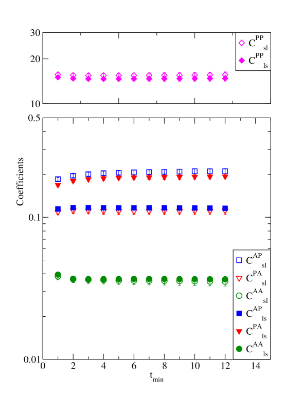
Figure 6: Comparison of $ls$ and $sl$ coefficients for all the pion correlators at $\kappa=0.1575$.

While the calculation of $C_{ss}$ is mandatory, in the literature (e.g.,alikhan ; orthprd ) $C_{sl}$ (corresponding to smeared sink and local source) has often been approximated by $C_{ls}$ and use $C_{ls}^{2}/C_{ss}$ to calculate $C_{ll}$. Since we have performed calculations with both local sink - smeared source ($ls$) and smeared source - local sink ($sl$) combinations, we can check the validity of this approximation . In Fig. 6 we plot $C_{ls}$ and $C_{sl}$ at $\kappa=0.1575$ for the all four pion correlators as functions of $t_{\rm min}$. Solid symbols are $ls$ and empty symbols are $sl$ correlators. As seen in the figure, all coefficients show decent plateau behavior. The data shown are at the respective optimum values of the smearing size parameter $s_{0}$ for each operator ($s_{0}=6$ for PP, $s_{0}=3$ for AA, AP and PA). While for the PP and the AA correlators, one should compare their respective $ls$ and $sl$ correlators, for the asymmetric correlators one should compare $C^{AP}_{ls}$ with $C^{PA}_{sl}$ and $C^{AP}_{sl}$ with $C^{PA}_{ls}$. As the figure also shows, it is grossly wrong to approximate $C^{AP}_{ls}$ by $C^{AP}_{sl}$ and similarly for PA. Actually the difference between $C^{AP}_{ls}$ and $C^{AP}_{sl}$ or between $C^{PA}_{ls}$ and $C^{PA}_{lsl}$ is significant, it is smearing size dependent and in this case it is about 50%. However, when one compares the correct quantities, i.e., $C^{AP}_{ls}$ and $C^{PA}_{sl}$, their central values differ by about 5%, while the central values of $C^{AP}_{sl}$ and $C^{PA}_{ls}$ differ by almost 10%. The difference between $ls$ and $sl$ coefficients for the case of the AA is the least (about 3%) while for PP it is about 5%.

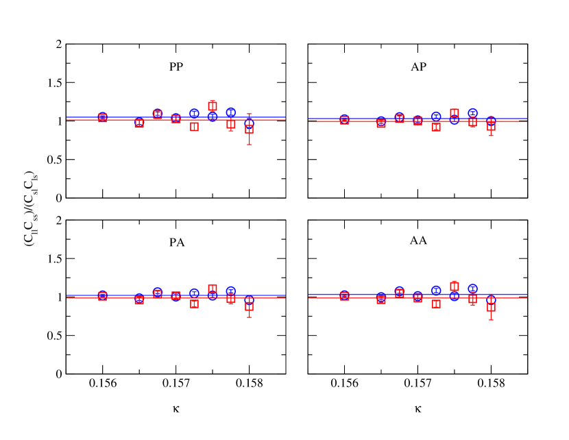
Figure 7: $C_{ll}C_{ss}/C_{sl}C_{ls}$ for all four pion operators as function of $\kappa$. This ratio should be equal to unity. The blue circles (red squares) represent data where the pion mass is determined from the PP (AA) correlator.

In Fig. 7 we show $C_{ll}C_{ss}/C_{sl}C_{ls}$ for all four pion correlators as function of $\kappa$. This ratio should be equal to unity. The circles (squares) represent data where the pion mass was determined from the PP (AA) correlator. The straight lines represent average values of the respective ratios. They are very close to unity (within a few percent). While the squares (pion mass taken from AA) show more fluctuation, the average is almost unity; the circles (mass taken from PP) are more stable, but their average shows a few percent bias above unity in all the four correlators. This general character is displayed in all the results of the derived quantities we have obtained, viz., data where $m_{\pi}$ was determined from AA show more fluctuation than the data where $m_{\pi}$ was determined from PP, but show the correct general trend, in particular seem to show less finite size effect (discussed later).

Before we end the discussion on the details of the implementation of the gaussian smearing, we present two figures to illustrate two particular features of the smearing. In Fig. 8 we show an example of oversmearing for the $ls$ PA correlator at $\kappa=0.15675$. While $s_{0}=1$ data look slightly undersmeared (albeit producing a decent plateau), $s_{0}=3$ completely destroys the plateau. $s_{0}=2$ produces a very stable plateau and has been accepted as the optimum value for this correlator, but the best value could have been somewhere between $s_{0}=1$ and $2$ (also please notice the significant difference between the $m_{\pi}$ values taken from the plateaux at $s_{0}=1$ and $2$). Our choice of $s_{0}=2$ for this correlator at this $\kappa$ is also dependent on the proper behavior (i.e. existence of stable plateau) of the other two smearing combinations, viz., $sl$ and $ss$ of the PA correlator at $\kappa=0.15675$.

Fig. 9 plots $am_{\pi}$ (computed from $ls$ AA correlator) versus $t_{\rm min}$ at $\kappa=0.1565$ for $s_{0}=1$ to $5$. The curious thing to observe in the plot is the crossing of the lines approximately at $t_{\rm min}=6$ indicating that $am_{\pi}$ is independent of $s_{0}$ for the fits using $t_{\rm min}=6$. One may conclude that the higher state contributions to the correlator are nearly absent at the crossing point and hence the value of $am_{\pi}$ at the crossing is fairly accurate. This kind of crossing does not take place always, but can be used whenever it does. Such a behavior was observed and discussed in the context of static quark potential with gauge field smearing in Ref. ape .

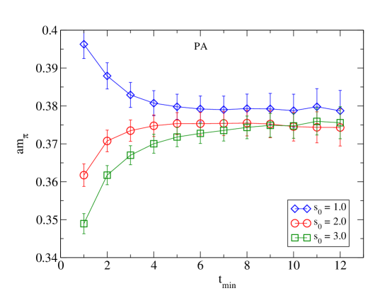
Figure 8: Example of oversmearing for the $ls$ PA correlator at $\kappa=0.15675$. The lines are just to guide the eye.

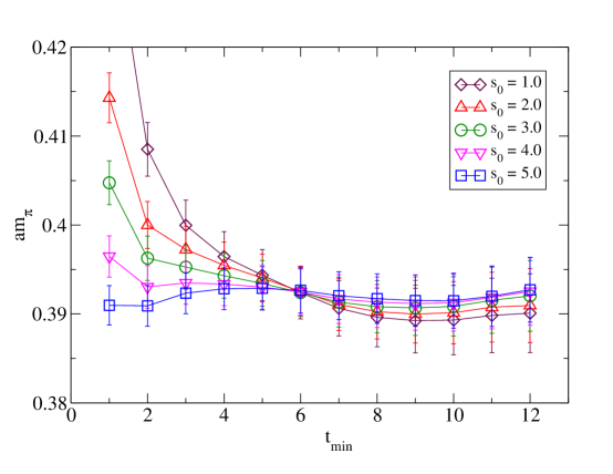
Figure 9: Crossing of $am_{\pi}$ determined from the AA correlator as function of $t_{\rm min}$ for different smearing size parameter $s_{0}$ at $\kappa=0.1565$. The lines are just to guide the eye.

The analysis for the rho correlator VV is done in a similar way, except that it was less tedious because VV was the only correlator we considered.

VII Results for the pion: $am_{\pi}$, $aF_{\pi}$ and $am_{q}$

We present in Table 3 all the results related to the pion. The results are presented in units of the lattice constant $a$. The results are put in two groups depending on whether $am_{\pi}$ is determined from the PP or the AA correlator, as described in the above section (Sec. VI). In each group, results have been presented for both the local (unsmeared) correlators and the smeared correlators. In each of these cases, as explained in Sec III, there are three ways each to evaluate $aF_{\pi}$ and the PCAC quark mass $am_{q}$.

$\kappa$	Observables		$am_{\pi}$ from PP		$am_{\pi}$ from AA
			with smearing	without smearing	with smearing	without smearing
	$am_{\pi}$		0.4503(16)	0.4522(19)	0.4506(28)	0.4513(32)
		$AA$	0.06698(87)	0.06628(87)	0.06711(83)	0.06615(82)
	$am_{q}$	$AP$	0.06744(40)	0.06574(30)	0.06764(52)	0.06570(43)
0.156		$PA$	0.06855(159)	0.06672(156)	0.06873(161)	0.06672(163)
		$AA$	0.09029(117)	0.09107(124)	0.09037(125)	0.09068(126)
	$aF_{\pi}$	$AP$	0.09090(91)	0.09033(90)	0.09109(131)	0.09006(108)
		$PA$	0.09239(202)	0.09168(200)	0.09256(207)	0.09145(196)
	$am_{\pi}$		0.3974(17)	0.3956(26)	0.3929(24)	0.3895(36)
		$AA$	0.05212(77)	0.05224(79)	0.05205(79)	0.05145(80)
	$am_{q}$	$AP$	0.05251(46)	0.05293(27)	0.05307(43)	0.05257(29)
0.1565		$PA$	0.05146(139)	0.05117(147)	0.05179(158)	0.05087(143)
		$AA$	0.07800(117)	0.07809(139)	0.07687(122)	0.07584(145)
	$aF_{\pi}$	$AP$	0.07859(97)	0.07913(93)	0.07838(80)	0.07748(104)
		$PA$	0.07701(194)	0.07650(222)	0.07650(217)	0.07498(217)
	$am_{\pi}$		0.3735(17)	0.3780(20)	0.3746(27)	0.3781(44)
		$AA$	0.04655(93)	0.04665(83)	0.04710(80)	0.04666(82)
	$am_{q}$	$AP$	0.04810(36)	0.04661(29)	0.04844(42)	0.04655(34)
0.15675		$PA$	0.04725(150)	0.04635(139)	0.04763(146)	0.04597(148)
		$AA$	0.07486(150)	0.07713(150)	0.07583(130)	0.07716(174)
	$aF_{\pi}$	$AP$	0.07735(97)	0.07706(105)	0.07799(106)	0.07697(140)
		$PA$	0.07598(229)	0.07662(223)	0.07669(223)	0.07601(259)
	$am_{\pi}$		0.3457(18)	0.3456(27)	0.3439(32)	0.3426(50)
		$AA$	0.04056(77)	0.04006(83)	0.04060(76)	0.03963(82)
	$am_{q}$	$AP$	0.04118(40)	0.04007(28)	0.04129(55)	0.04006(28)
0.157		$PA$	0.04052(153)	0.03933(152)	0.04044(161)	0.03986(135)
		$AA$	0.07138(137)	0.07179(165)	0.07109(140)	0.07074(186)
	$aF_{\pi}$	$AP$	0.07249(99)	0.07181(97)	0.07230(130)	0.07150(111)
		$PA$	0.07131(258)	0.07049(275)	0.07082(280)	0.07114(253)
	$am_{\pi}$		0.3147(20)	0.3194(25)	0.3122(26)	0.3030(48)
		$AA$	0.03491(64)	0.03520(70)	0.03500(65)	0.03367(75)
	$am_{q}$	$AP$	0.03431(33)	0.03355(30)	0.03451(36)	0.03334(32)
0.15725		$PA$	0.03632(126)	0.03516(122)	0.03656(127)	0.03490(127)
		$AA$	0.06762(129)	0.06986(157)	0.06731(129)	0.06513(170)
	$aF_{\pi}$	$AP$	0.06648(86)	0.06658(90)	0.06636(93)	0.06450(99)
		$PA$	0.07037(237)	0.06979(245)	0.07032(233)	0.06751(256)
	$am_{\pi}$		0.2876(20)	0.2890(29)	0.2893(32)	0.3000(61)
		$AA$	0.02663(81)	0.02618(85)	0.02706(77)	0.02740(78)
	$am_{q}$	$AP$	0.02896(36)	0.02804(30)	0.02933(61)	0.02814(33)
0.1575		$PA$	0.02697(125)	0.02615(122)	0.02731(136)	0.02630(112)
		$AA$	0.06073(197)	0.06089(216)	0.06153(176)	0.06440(202)
	$aF_{\pi}$	$AP$	0.06604(120)	0.06521(122)	0.06670(146)	0.06613(125)
		$PA$	0.06150(288)	0.06082(294)	0.06212(301)	0.06181(271)
	$am_{\pi}$		0.2481(38)	0.2554(39)	0.2360(49)	0.2345(76)
		$AA$	0.02173(58)	0.02233(60)	0.02116(70)	0.02122(61)
	$am_{q}$	$AP$	0.02039(36)	0.02081(28)	0.02116(42)	0.02167(42)
0.15775		$PA$	0.02298(94)	0.02289(100)	0.02270(126)	0.02306(124)
		$AA$	0.05523(162)	0.05726(169)	0.05325(189)	0.05279(187)
	$aF_{\pi}$	$AP$	0.05182(100)	0.05337(91)	0.05327(99)	0.05392(109)
		$PA$	0.05840(240)	0.05871(268)	0.05714(337)	0.05737(329)
	$am_{\pi}$		0.2278(28)	0.2255(53)	0.2142(81)	0.2051((167)
		$AA$	0.01481(67)	0.01462(69)	0.01452(75)	0.01369(81)
	$am_{q}$	$AP$	0.01348(44)	0.01380(44)	0.01435(62)	0.01431(52)
0.158		$PA$	0.01592(122)	0.01566(125)	0.01664(119)	0.01564(128)
		$AA$	0.04658(222)	0.04587(225)	0.04454(244)	0.04239(261)
	$af_{\pi}$	$AP$	0.04239(141)	0.04330(148)	0.04404(166)	0.04432(170)
		$PA$	0.05006(395)	0.04915(401)	0.05105(365)	0.04843(406)

Table 3: Results for $am_{\pi}$, $aF_{\pi}$ and PCAC quark mass $am_{q}$.

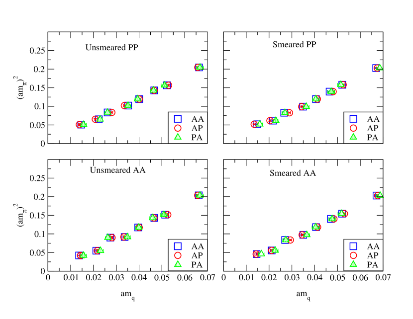
Figure 10: $(am_{\pi})^{2}$ obtained from unsmeared and smeared PP and AA correlators versus different evaluations of $am_{q}$.

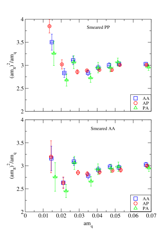
Figure 11: The ratio $(am_{\pi})^{2}/(am_{q})$ obtained from smeared PP and AA correlators versus different evaluations of $am_{q}$.

The errors presented in Table 3 are statistical errors calculated by the single-omission jackknife method calculated from 200 jackknife bins. In general, the $am_{\pi}$ errors increase as $\kappa$ increases. These errors are systematically more for the pion masses determined from the AA correlator than from the PP correlator and within each group more for the determination from the unsmeared correlators than the smeared correlators. $aF_{\pi}$ is the most inaccurate quantity presented in Table 3. In each group, both $aF_{\pi}$ and $am_{q}$ have the least errors when the correlator AP is used; they are the most inaccurate when the correlator PA is used. For determination of quantities when pion mass was determined from the unsmeared AA correlator, at times the quality of the plateau was poor resulting in inaccurate data; this was especially true for $\kappa=0.15725$ and $0.1575$.

Fig. 10 plots $(am_{\pi})^{2}$ determined from unsmeared and smeared PP and AA correlators versus different evaluations of $am_{q}$. Except for the data points with the lowest pion and quark masses, the rest appears to be roughly consistent with the lowest order (LO) chiral perturbation theory ($\chi PT$). As already mentioned, out of the four plots in Fig. 10, the bottom left plot (pion mass from unsmeared AA) looks the worst. In all cases, the PCAC quark mass $am_{q}$ determined from the AP and the PP correlator (shown in plots as AP: open circles) has the least error.

Any departure from LO $\chi PT$ shows up in the behavior of the ratio $(am_{\pi})^{2}/(am_{q})$, called the chiral ratio below, as a function $am_{q}$. This is plotted for the data obtained only from the smeared correlators in Fig. 11. Firstly we need to separate any effect of finite size effect on the masses before discussing the chiral behavior. We are quite confident that for the values of $\kappa$ from 0.156 to 0.1575, there is negligible finite size effect on these masses, because data, consistent with our numbers, are available in previous literature at some of these $\kappa$ values at larger volumes (see below for discussion and references), For the masses at $\kappa=0.15775$, our guess is that for different operators there is a difference in finite size effect. From both the Figs. 10 and 11, it seems that there is a little bit of finite size effect for the pion mass at this $\kappa$, but more with pion mass determined from PP than AA, because in the upper plot of Fig. 11 there is an upward trend at this point. This is not to be taken as an effect from next-to-leading order (NLO) $\chi PT$ because with standard values of low energy effective (LE) constants of $\chi PT$ obtained from other studies (both on the lattice and otherwise), there should not be an upward trend of the ratio (as seen in the upper plot here) at this pion mass.

Difference in the finite size effect on the pion mass calculated from different operators is an interesting observation and to the best of our knowledge has not been discussed in the literature before. It is fair to say that this is not an unexpected behavior. However, what is also interesting is that the generally accepted noisier operator AA produces less finite size effect.

If our data see only the LO $\chi PT$, then the ratio should be a perfect straight line parallel to the $am_{q}$ axis. If we believe our error bars, there is a significant downward trend of the ratio from the larger quark masses to the smaller quark masses (more pronounced with the AA and PA quark masses). For the lower plot of Fig. 11 this trend continues and intensifies to the second last point from the left (at $\kappa=0.15775$) which can only be an effect from higher order terms of $\chi PT$.

The left-most point (at $\kappa=0.158$) definitely has a significant finite size effect as we can compare our data with evaluations on larger volumes (see below). Even at this point, the pion mass determined from the smeared AA correlator has smaller finite size effect as apparent from the figure. We also like to point out that the finite size effects, its dependence on the pion operators etc have nothing to do with smearing or the smearing size milcw . The same effects are also visible from similar data from unsmeared operators (although not plotted in Fig. 11, but available in Table 3 and Fig. 10).

Fig. 12 plots $aF_{\pi}$ versus $am_{q}$ in way similar to Fig. 10. The bottom left plot where the pion mass is determined from unsmeared AA correlator has the most inaccuracies. The main difference with the $am_{\pi}^{2}$ plot is that the finite size effect at $\kappa=0.15775$ and 0.158 is now quite severe. This is consistent with $\chi PT$ which predicts four times larger (and opposite in sign) finite size effect for $aF_{\pi}$ as compared to $am_{\pi}^{2}$ cola . The behavior of $aF_{\pi}$ with $am_{q}$ using the AA operator (squares) show the most continuous behavior, even though these have larger error-bars compared to the $am_{q}$ data computed from the AP correlator.

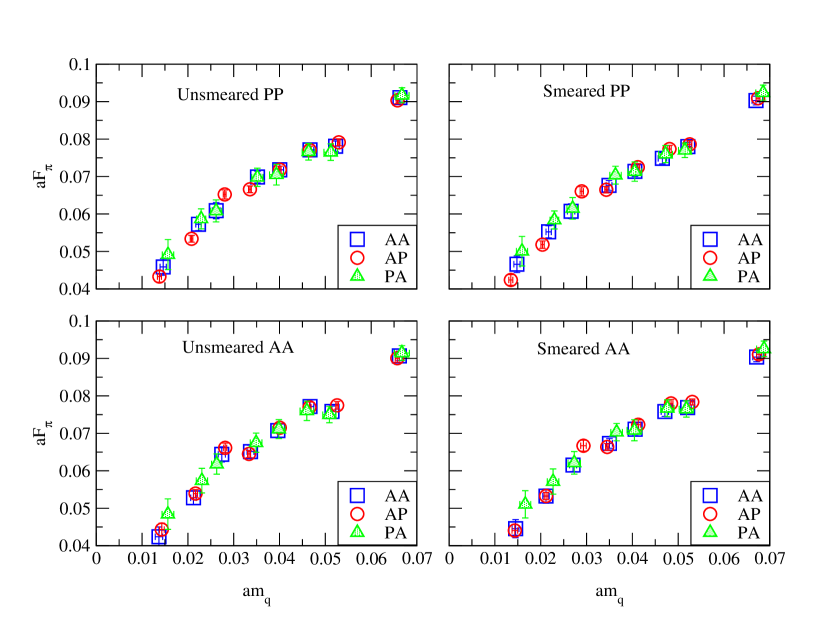
Figure 12: $aF_{\pi}$ obtained from unsmeared and smeared PP and AA correlators versus different evaluations of $am_{q}$.

VII.1 Chiral behavior

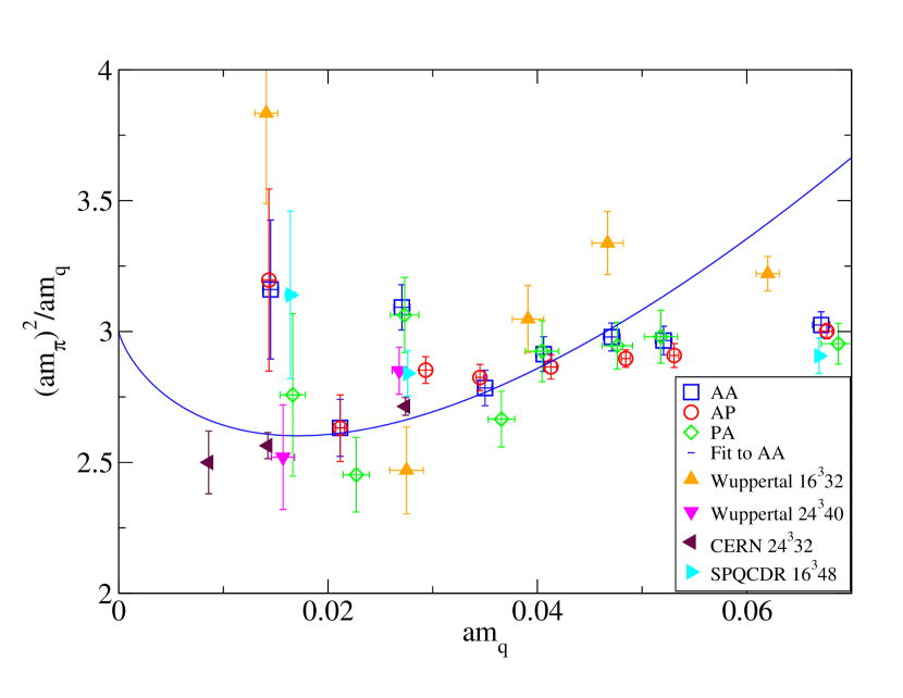
Figure 13: The chiral ratio $(am_{\pi})^{2}/am_{q}$ obtained from smeared AA correlator versus different evaluations of $am_{q}$. Figure includes data from other work at same or larger volume and a suggestive NLO chiral plot.

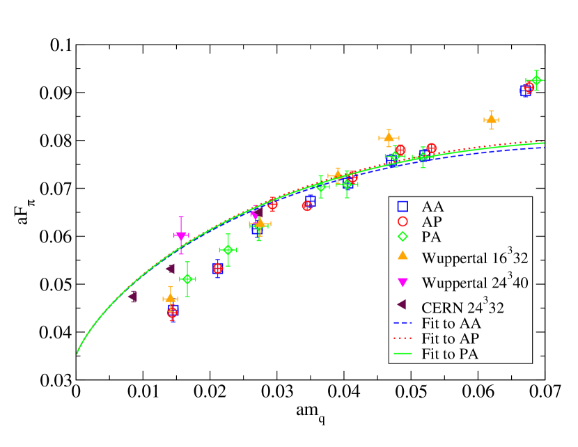
Figure 14: $aF_{\pi}$ obtained from smeared AA correlator versus different evaluations of $am_{q}$. Figure includes data from other work at same or larger volume and a suggestive NLO chiral plot

We have plotted in Figs. 13 and 14 the whole content of the bottom figures of Fig. 11 and 12 respectively (data from smeared AA correlator only, represented by open symbols) along with (unimproved) $N_{F}=2$ Wilson data at $\beta=5.6$ from Ref. orthprd ($16^{3}32$ and $24^{3}40$), Ref. besirevic ($16^{3}48$) and Ref. deldebbio2 ($24^{3}32$) (data from others represented by different filled symbols). These figures also show NLO $\chi PT$ leut plots

$$\frac{(am_{\pi})^{2}}{am_{q}} = 2aB\left[1-\frac{m_{q}B}{16\pi^{2}F^{2}}{\rm ln}\frac{\Lambda_{3}^{2}}{2m_{q}B}\right]$$ (30)

$$aF_{\pi} = aF\left[1+\frac{m_{q}B}{8\pi^{2}F^{2}}{\rm ln}\frac{\Lambda_{4}^{2}}{2m_{q}B}\right]$$ (31)

with $aF=0.035$, $aB=1.5$. With these values of $aF$ and $aB$ as input we actually could fit our data (for $am_{q}^{AA}$, represented by squares) for both the chiral ratio and $aF_{\pi}$. For the chiral ratio, the fits include points from $\kappa=0.15675,0.157,0.15725$ and 0.15775. The point at $\kappa=0.1575$ is excluded from the fit because of systematic fluctuations. The fit to the $aF_{\pi}$ data is also done with the AP and PA quark masses in a similar range of data. The values of $a\Lambda_{3}$ and $a\Lambda_{4}$ that come out of the fits are: $a\Lambda_{3}=0.374(7)$, $a\Lambda_{4}=0.813(11)$.

Let us state categorically that the chiral NLO plots are not to be taken as serious fits, they are shown more to understand our data and where the data of other works (with same parameters), especially on larger volumes, are in relation to our data and the chiral NLO plots. Firstly, the NLO fits for both the chiral ratio and the $aF_{\pi}$ are done with the same input values of $aF$ and $aB$. Secondly, the fit to the chiral ratio is done with $am_{q}^{AA}$ (denoted by open squares) and nearly goes through all the points of the fit, Our other data points with $am_{q}^{AP}$ (circles, with their small error bars) and with $am_{q}^{PA}$ (diamonds, with large error bars) are also close to this NLO curve. Thirdly, the data points on larger lattices (at $\kappa=0.158$ by deldebbio2 ; orthprd , at $\kappa=0.1575$ by deldebbio2 lie very close to both the NLO fits (Figs. 13 and 14). The data with the smallest quark mass from deldebbio2 at $\kappa=0.15825$ has a large error bar on the chiral ratio plot, however, on the $aF_{\pi}$ plot looks very close to the NLO fit. The errors for the $16^{3}$ data from orthprd ; besirevic are calculated by us from their quoted pion and quark mass data by quadrature (Ref. besirevic has no $F_{\pi}$ data either). Some of these $16^{3}$ data look a bit erratic, especially from orthprd . Finally, probably because of large finite size effect on $aF_{\pi}$, the numerical data computed on relatively smaller lattices (including ours) tend to have a larger downward bend than is consistent with acceptable values for the low energy constants. However, our fits with $aF$ and $aB$ as inputs, done from $\kappa=0.1565$ to 0.1575, for all the quark masses $am_{q}^{AA}$, $am_{q}^{AP}$ and $am_{q}^{PA}$ give a reasonable fit with the evaluations upto $\kappa=0.15825$ on larger lattices staying very close to this explorative NLO fit.

At this point if we look back at the Fig. 10 and take a closer look, we discover that this figure is not consistent with LO $\chi PT$, because data at larger masses do not go though the origin in a straight line. The data in all the plots of Fig. 10 actually have a small bend.

VII.2 Comparison of VWI and AWI masses

In all the Tables and Figures above, we have presented results for the quark mass from the PCAC relation, $am_{q}^{AWI}$, which is devoid of ${\cal O}(a)$ effects because the PCAC relation guarantees that the square of the pion mass vanishes as the quark mass approaches zero. $\chi PT$ can also be made consistent with this, once the quark masses used there are the PCAC masses ss .

Traditionally, one also defines the VWI (vector Ward Identity) quark mass as

$$am^{VWI}_{q}=\frac{1}{2}\left(\frac{1}{\kappa}-\frac{1}{\kappa_{c}}\right),$$ (32)

where $\kappa\rightarrow\kappa_{c}=1/8=0.125$ in the chiral limit for the free theory ($U_{x\mu}=1$).

At the tree level, this definition takes care of the ${\cal O}(a)$ additive quark mass. However, at the quantum level, $m^{VWI}_{q}$ should be devoid of ${\cal O}(a)$ effects only approximately. The effect should be worse at smaller values of $\beta$ with a larger lattice constant $a$.

The behaviour of $(am_{\pi})^{2}$ as function of $\frac{1}{\kappa}$ is shown in Fig. 15 for pion masses determined from unsmeared and smeared PP and AA correlators. Although the data from unsmeared AA correlators show more fluctuations, straight lines fits excluding $\kappa=0.158$ (because of sizable finite size effects) are possible in all cases giving a determination of $\kappa_{c}$. The values of $\kappa_{c}$ obtained are as follows: (i) 0.15858(3) (PP-smeared), (ii) 0.15862(4) (PP-unsmeared), (iii) 0.15854(4) (AA-smeared), and (iv) 0.15855(6) (AA-unsmeared). For the same lattice volume and $\beta$, SESAME and T$\chi$L Collaboration tlqcd obtained $\kappa_{c}=0.158493(16)$.

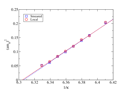
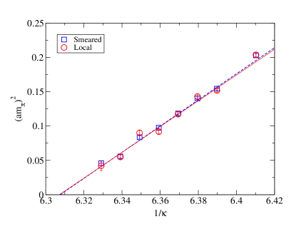
Figure 15: $(am_{\pi})^{2}$ obtained from unsmeared and smeared PP (left) and AA (right) correlators versus $\frac{1}{\kappa}$.

The values of $am^{VWI}_{q}$ calculated using Eq. (32) are presented in Table 4.

$\kappa$	$am_{\pi}$ from PP		$am_{\pi}$ from AA
	with smearing	without smearing	with smearing	without smearing
0.156	0.05215(55)	0.05294(75)	0.05135(75)	0.05155(126)
0.1565	0.04191(55)	0.04270(75)	0.04111(75)	0.04131(126)
0.15675	0.03681(55)	0.03761(75)	0.03601(75)	0.03621(126)
0.157	0.03173(55)	0.03253(75)	0.03094(75)	0.03113(126)
0.15725	0.02667(55)	0.02746(75)	0.02587(75)	0.02607(126)
0.1575	0.02162(55)	0.02242(75)	0.02083(75)	0.02102(126)
0.15775	0.01659(55)	0.01738(75)	0.01579(75)	0.01599(126)
0.158	0.01157(55)	0.01237(75)	0.01078(75)	0.01098(126)

Table 4: $am_{q}^{VWI}$ in dependence of $\kappa$.

We note that $m_{q}^{AWI}$ has no ${\cal O}(a)$ scaling violation whereas $m_{q}^{VWI}$ has some remaining ${\cal O}(a)$ scaling violation. Fig. 16 plots the deviation of $m_{q}^{VWI}$ from $m_{q}^{AWI}$ as a function of $\frac{1}{\kappa}$. We notice small fluctuations (a few percent) around a normalization factor of approximately 0.78 (i.e., $m_{q}^{AWI}\approx 0.78m_{q}^{VWI}$). Even at $\kappa=0.158$ where the fluctuation is maximum shows a deviation of about 6% from the normalization. If these deviations are any signature, scaling violations may be small in our case, This is to be expected at our lattice scale $a\approx 0.08{\rm fm}$ ($a^{-1}\sim 2.45{\rm GeV}$) qcd_paper1 .

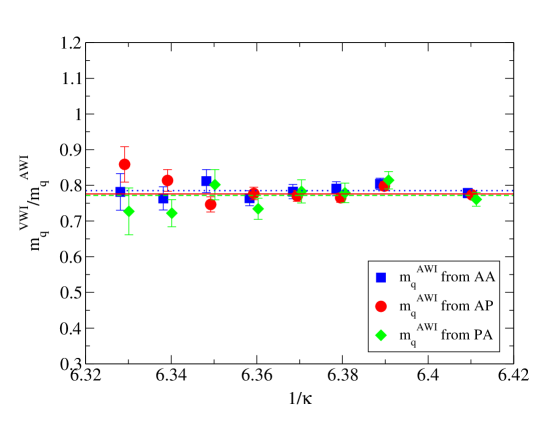
Figure 16: Deviation of of $m_{q}^{VWI}$ from $m_{q}^{AWI}$ (some of the data slightly shifted horizontally for clarity).

VIII Results for the Rho: $am_{\rho}$, $aF_{\rho}$ and different ratios

Table 5 presents our results for the rho mass and the decay constant in lattice units for all the $\kappa$ values of our simulation. The errors are again the single-omission jackknife errors computed from 200 jackknife bins. In general the errors are more for larger $\kappa$ and for data from unsmeared correlators (especially for $am_{\rho}$). With the range of pion masses reached in our simulations, $2m_{\pi}>m_{\rho}$ was always satisfied and there was no complication in the investigation of the rho correlator.

The data for $am_{\rho}$ is plotted in Fig. 17 as a function of $am_{q}^{AP}$. For clarity of the figure, other quark masses are not shown in this figure (even in this case, there are four different PCAC quark masses depending on whether the pion mass was determined from unsmeared or smeared PP or AA correlators). The straight line fits shown in the figure exclude points for the two extreme $\kappa$ and for $\kappa=0.15725$ (appearing to have a systematic error) and lead to a value close to the physical rho mass on chiral extrapolation. As expected, the lowest rho mass at $\kappa=0.158$ has some finite size effect.

Fig. 18 shows three ratios $F_{\pi}/F_{\rho}$, $1/f_{\rho}=F_{\rho}/m_{\rho}$ and $F_{\pi}/m_{\rho}$ obtained from smeared correlators versus PCAC quark masses. The left (right) figure shows the dependence of these ratios on AA, AP and PA quark masses when the pion mass was determined from the smeared PP (AA) correlator. The drop at small quark masses in the ratios $F_{\pi}/F_{\rho}$, and $F_{\pi}/m_{\rho}$ are mainly attributable to the most significant finite size effect of $F_{\pi}$. The quantity in the middle $1/f_{\rho}=F_{\rho}/m_{\rho}$ is actually a ratio of the other two ratios and with the elimination of $F_{\pi}$ cancels out whatever finite size effects of $F_{\rho}$ and $m_{\rho}$.

With phenomenological inputs of $m_{\rho}=771.1MeV$, $F_{\pi}=92.4MeV$ and $\sqrt{2}F_{\rho}=216MeV$, Fig. 18 also enables approximate estimations of the renormalization constants $Z_{V}$ and $Z_{A}$ associated with $F_{\rho}$ and $F_{\pi}$ respectively. Fit to all points of the ratio $1/f_{\rho}=F_{\rho}/m_{\rho}$ leads to $Z_{V}=0.659(2)$ and a similar fit to points corresponding to $\kappa=$0.1565 to 0.15725 for the ratio $F_{\pi}/m_{\rho}$ leads to $Z_{A}=0.76(1)$. These are remarkably close to the values quoted in deldebbio1 ; besirevic .

$\kappa$	$am_{\rho}$		$aF_{\rho}$
	with smearing	without smearing	with smearing	without smearing
0.156	0.5365(23)	0.5409(32)	0.1577(17)	0.1631(24)
0.1565	0.4935(25)	0.4890(41)	0.1460(17)	0.1443(27)
0.15675	0.4730(27)	0.4765(43)	0.1427(16)	0.1460(28)
0.157	0.4516(28)	0.4510(50)	0.1369(13)	0.1385(30)
0.15725	0.4170(45)	0.4202(56)	0.1266(31)	0.1300(30)
0.1575	0.4069(34)	0.4098(70)	0.1290(25)	0.1323(40)
0.15775	0.3811(70)	0.3847(82)	0.1175(47)	0.1221(44)
0.158	0.3675(71)	0.3697(122)	0.1103(99)	0.1130(62)

Table 5: $am_{\rho}$ and $aF_{\rho}$ from smeared and unsmeared VV correlators for all the values of $\kappa$

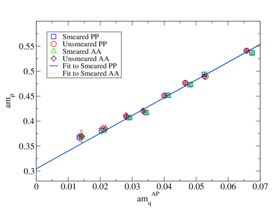
Figure 17: $am_{\rho}$ obtained from unsmeared and smeared PP and AA correlators versus $am_{q}^{AP}$.

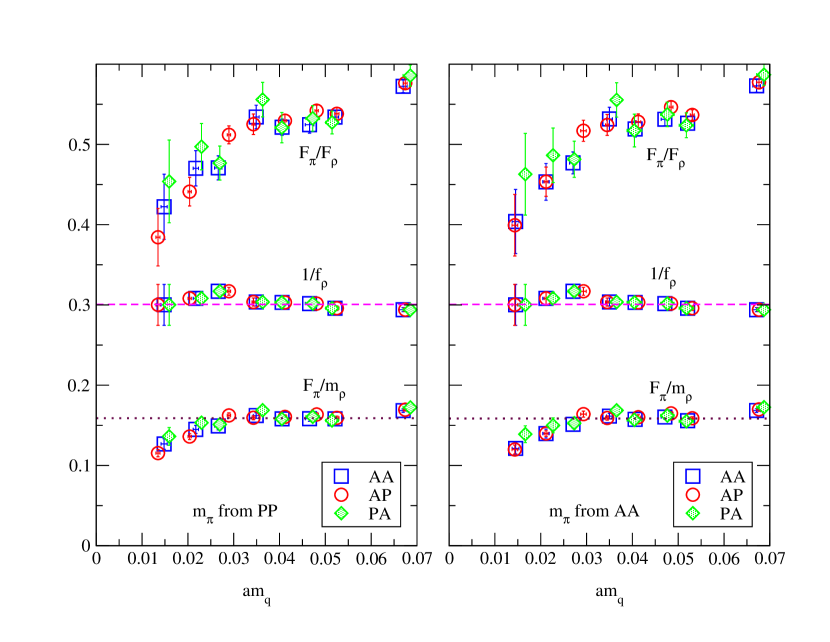
Figure 18: $F_{\pi}/F_{\rho}$, $1/f_{\rho}=F_{\rho}/m_{\rho}$ and $F_{\pi}/m_{\rho}$ obtained from smeared correlators versus different evaluations of $am_{q}$.

IX Summary and conclusions

Due to recent theoretical, algorithmic and technological advances, Lattice QCD with Wilson fermions has entered a very active phase. We have planned on a detailed lattice QCD investigation with Wilson and Wilson-type fermions. In this work we have taken the first step towards addressing the issues that are encountered probing the chiral regime of lattice QCD systematically. Here, our emphasis is to have fully dynamical simulations at an extensive set of $\kappa$ values and study accurate determinations of the masses and decay constants in as many ways as possible. We employ standard (unimproved) Wilson gauge and fermion actions with 2 fully dynamical light quark flavors on $16^{3}32$ lattice, $\beta=6/g^{2}=5.6$ at 8 values of bare quark masses (corresponding to fermionic hopping parameter $\kappa=0.156,~{}0.1565,~{}0.15675,~{}0.157,~{}0.15725,~{}0.1575,~{}0.15775,~{}0.158$). The lattice scale reached is respectable and $a\sim 0.08$ fm ($a^{-1}\sim 2.45$ GeV) qcd_paper1 .

In order to accurately extract the mass gap from the asymptotic behavior of Euclidean time correlation functions, various smearing techniques applied to the hadron operator have been employed in the literature. Among them, gaussian smearing which can be motivated from conceptually simple considerations can be implemented in numerical simulations in a simple and straight forward manner. To assess the strengths and weaknesses of the gaussian smearing, we have carried out an extensive study that employs local-smear, smear-local and smear-smear sink-source combinations at many values of the smearing size parameter $s_{0}$.

At each value of the smearing size, to extract meson observables, a variety of correlation functions are measured. Using the pseudoscalar and the fourth component of the axial vector densities denoted by P and A respectively, for the pion, PP, AA, AP and PA correlators are used since both P and A carry quantum numbers of pion. We have extracted mass gaps and amplitudes (coefficients of the correlators) for the smearing radius $s_{0}$ ranging from 1 to 8 in steps of 1 for all these corelation functions for all the three smearing combinations. At each $\kappa$, we find the optimum smearing size $s_{0}$ for each correlator type; the optimum $s_{0}$ in general is different for different correlators types and also varies with $\kappa$. In the case of pion, we do not detect any systematics in the optimum choice of $s_{0}$ as a function of $\kappa$ as is seen from Table 3 except that the optimum smearing size is smaller for AA, AP and PA than for PP. One should also be cautious about oversmearing. In the case of rho we find that $s_{0}$ gradually increases as $\kappa$ increases.

We have also carried out extensive calculations with local operators in order to quantify the systematic effects in the determination of masses and decay constants.

We have obtained the pion masses from PP and also from AA correlators. These masses are then used to determine the coefficients for all the correlators. In each case we obtained pion decay constant and quark masses using AA, AP and PA correlators. The values obtained using AP (PA) correlator usually has the lowest (highest) errors.

The general conclusion regarding the use of the different correlator types PP, AA, AP and PA appears to be the following: whenever the axial vector operator is at the source (i.e., AA or PA), the data (be it the pion mass, decay constant or the quark mass) seems to have more noise and statistical errors. However, despite that, these data seem to have a better general trend overall (be it consistency check for smearing (Fig. 7), comparison with the VWI quark mass (Fig. 16) or chiral trends (Figs. 13 and 14), they also seem to have significantly less finite volume effects.

The quantities derived from correlators with the psedoscalar operator (i.e., PP and AP) at the source seem to have the least statistical errors, however, they seem to carry some systematic errors and definitely show signs of stronger finite size effects at larger $\kappa$ values.

Although we have performed a lattice QCD investigation with fully dynamical quarks at a host of values of $\kappa$, we do not have nearly enough data points or small enough quark masses to have a reliable chiral extrapolation. Let us make it very clear that although it is one of our ultimate aims, in this paper it was not our intention either. Given our emphasis on other aspects, e.g., study of smearing in a very detailed manner or comparison of all pion correlators, we still can make a few interesting observations regarding chiral trend of our data. In both the behaviors of $aF_{\pi}$ and the chiral ratio $(am_{\pi})^{2}/(am_{q})$ versus $am_{q}$, we see indication of departure from LO $\chi PT$. The chiral ratio has a slope downwards in the range of $am_{q}$ = 0.05 - 0.025 and our data is more consistent with NLO $\chi PT$ than LO. Data from other works (with same parameters as ours) done at larger volumes are also consistent with this chiral trend including points at smaller quark masses upto $am_{q}\leq 0.015$. The chiral ratios at $\kappa=0.158$ with $16^{3}32$ lattices (from all collaborations including ours) show significant finite size effect.

The data for $aF_{\pi}$ is also consistent with NLO $\chi PT$ in the range $am_{q}$ = 0.05 - 0.03. The faster decrease with respect to $am_{q}$ at $\kappa=0.15775$ and 0.158 is clearly due to, and in accordance with $\chi PT$ finite size effects. This is again corroborated with the simulations done at the same and larger volumes for the same $\kappa$ range.

We have studied the deviation of $am_{q}^{VWI}$ from $am_{q}^{AWI}$ as a function of $\kappa$. We note that $am_{q}^{AWI}$ has no ${\cal O}(a)$ scaling violation whereas $am_{q}^{VWI}$ has some remaining ${\cal O}(a)$ scaling violations. We have noticed small fluctuations (a few percent) around a normalization factor of approximately 0.78. If these deviations are any signature, scaling violations may be small in our case.

The dimensionless ratio $\frac{F_{\rho}}{m_{\rho}}$ is remarkably independent of $am_{q}$ in the range 0.07 - 0.015 and we can easily extract the constant value of this ratio $\approx 0.301$. Comparison with the physical value of this ratio (0.198) yields an estimate of $Z_{V}\approx 0.659$. The dimensionless ratio $\frac{F_{\pi}}{m_{\rho}}$ is approximately independent of $am_{q}$ in the range 0.055 - 0.03. The deviation from constancy for the smallest two values of $am_{q}$ is due to finite size effects. The constant value extracted for the ratio is 0.159. Comparison with the physical value of this ratio (0.120) yields an estimate of $Z_{A}\approx 0.76$. It is encouraging that the extracted values for both these renormalization constants (which are independent of the lattice scale) are in agreement with those extracted non-perturbatively on the lattice in Ref. deldebbio1 ; besirevic .

We find our initial results interesting and very encouraging. Simulations are underway utilizing significantly larger lattices and improved algorithms in order to further test the accessibility of chiral region to the naive Wilson action (both gauge and fermion sectors). It will be interesting to compare our results obtained with unimproved Wilson fermion and gauge action to that with improved actions, for example, Refs. clover ; domain ; twisted .

Appendix A Fourier Transform Trick for Sink Smearing

In this appendix, we follow the discussion in Ref. hauswirth . Generically we need to calculate

$$\sum_{{\bf x}}\langle{\cal O}^{\rm sink}({\bf x},t){\cal O}^{\rm source}({\bf x}_{0},t_{0})\rangle~{}.$$ (33)

Case I (local source, local sink) We have

$$\sum_{{\bf x}}\langle{\overline{\psi}}({\bf x},t)\Gamma\psi({\bf x},t){\overline{\psi}}({\bf x}_{0},t_{0})\Gamma\psi({\bf x}_{0},t_{0})\rangle~{}=~{}\sum_{\bf x}\langle{\rm Trace}~{}(S({\bf x},t;{\bf x}_{0},t_{0})\Gamma S({\bf x}_{0},t_{0};{\bf x},t)\Gamma)\rangle~{}$$ (34)

where $\Gamma$ denotes any of the sixteen Dirac matrices. The fermion propagator $S(x,y)$ is obtained by solving the equation

$$MS=\delta$$ (35)

where $M$ is the Dirac-Wilson operator.

Writing the coordinates explicitly, we have,

$$\sum_{{\bf x}_{1},t_{1}}M({\bf z}_{1},\tau;{\bf x}_{1},t_{1})~{}S({\bf x}_{1},t_{1};{\bf{\bf y}}_{1},0)~{}=~{}\delta_{{\bf z}_{1},{\bf{\bf y}}_{1}}~{}\delta_{\tau,0}~{}.$$ (36)

For the calculation of the meson propagator, Eq. (34), we need to calculate only $S({\bf x},t;{\bf x}_{0},t_{0})$ since $S({\bf x}_{0},t_{0};{\bf x},t)$ is trivially calculated from

$$S({\bf x}_{0},t_{0};{\bf x},t)~{}=~{}\gamma_{5}~{}S^{\dagger}({\bf x},t;{\bf x}_{0},t_{0})~{}\gamma_{5}~{}.$$ (37)

Case II (local source, smeared sink)

$${\cal O}^{\rm sink}~{} = ~{}\sum_{{\bf x}_{1}{\bf x}_{2}}~{}\phi({\bf x}_{1}-{\bf x})~{}\phi({\bf x}_{2}-{\bf x})~{}{\overline{\psi}}({\bf x}_{1},t)\Gamma~{}\psi({\bf x}_{2},t)$$

$${\cal O}^{\rm source}~{} = ~{}{\overline{\psi}}({\bf x}_{0},t_{0})\Gamma~{}\psi({\bf x}_{0},t_{0})~{}.$$ (38)

Now we have,

$$\sum_{{\bf x}}\sum_{{\bf x}_{1}{\bf x}_{2}}~{}\phi({\bf x}_{1}-{\bf x})~{}\phi({\bf x}_{2}-{\bf x})~{}\langle{\rm Trace}~{}S({\bf x}_{2},t;{\bf x}_{0},t_{0})~{}\Gamma\gamma_{5}S^{\dagger}({\bf x}_{1},t;{\bf x}_{0},t_{0})\gamma_{5}~{}\Gamma\rangle~{}.$$ (39)

Going to momentum space,

$$\phi({\bf x}_{1}-{\bf x}_{0})~{} = ~{}1/N~{}\sum_{{\bf k}_{1}}~{}e^{-i{\bf k}_{1}\cdot({\bf x}_{1}-{\bf x}_{0})}~{}{\tilde{\phi}}({\bf k}_{1}),$$

$$S({\bf x}_{2},t;{\bf x}_{0},t_{0})~{} = ~{}1/N~{}\sum_{{\bf k}_{3}}~{}e^{-i{\bf k}_{3}\cdot({\bf x}_{2}-{\bf x}_{0})}~{}{\tilde{S}}({\bf k}_{3},t)~{},~{}{\rm etc}.,$$ (40)

we get,

$$(1/N)^{4}~{}\sum_{{\bf k}}~{}{\tilde{\phi}}({\bf k})~{}{\tilde{\phi}}({\bf k})~{}\langle{\rm Trace}~{}{\tilde{S}}({\bf k},t)~{}\Gamma~{}\gamma_{5}~{}{\tilde{S}}^{\dagger}({\bf k},t)~{}\gamma_{5}~{}\Gamma\rangle~{}.$$ (41)

Need to calculate only ${\tilde{S}}({\bf k},t)$ and ${\tilde{\phi}}({\bf k})$.

Case III (smeared source, local sink)

$${\cal O}^{\rm source}~{} = ~{}\sum_{{\bf x}_{1}{\bf x}_{2}}~{}\phi({\bf x}_{1}-{\bf x}_{0})~{}\phi({\bf x}_{2}-{\bf x}_{0})~{}{\overline{\psi}}({\bf x}_{1},t_{0})\Gamma~{}\psi({\bf x}_{2},t_{0})$$

$${\cal O}^{\rm sink}~{} = ~{}{\overline{\psi}}({\bf x},t)\Gamma~{}\psi({\bf x},t)~{}.$$ (42)

Now we have,

$$\sum_{{\bf x}}~{}\sum_{{\bf x}_{1}{\bf x}_{2}}~{}\phi({\bf x}_{1}-{\bf x}_{0})~{}\phi({\bf x}_{2}-{\bf x}_{0})~{}\langle{\rm Trace}S({\bf x},t;{\bf x}_{1},t_{0})~{}\Gamma~{}\gamma_{5}S^{\dagger}({\bf x},t;{\bf x}_{2},t_{0})\gamma_{5}\Gamma\rangle~{}.$$ (43)

$$=\sum_{\bf x}~{}\langle{\rm Trace}{\cal S}({\bf x},t;{\bf x}_{0},t_{0})\Gamma\gamma_{5}{\cal S}^{\dagger}({\bf x},t;{\bf x}_{0},t_{0})\gamma_{5}~{}\Gamma\rangle$$ (44)

where

$${\cal S}({\bf x},t;{\bf x}_{0},t_{0})~{}=~{}\sum_{{\bf x}_{1}}~{}\phi({\bf x}_{1}-{\bf x}_{0})S({\bf x},t;{\bf x}_{1},t_{0})~{}.$$ (45)

Starting from Eq. (36),

$$\sum_{{\bf x}_{1}}M({\bf y},t_{y};{\bf x},t)~{}S({\bf x},t;{\bf x}_{1},0)~{}\phi({\bf x}_{1}-{\bf x}_{0})~{}=~{}\sum_{{\bf x}_{1}}\delta({\bf y}-{\bf x}_{1})~{}\phi({\bf x}_{1}-{\bf x}_{0})~{}\delta(t_{y}-0)~{}.$$ (46)

i.e.,

$$M({\bf y},t_{y};{\bf x},t)~{}{\cal S}({\bf x},t;{\bf x}_{0},0)~{}=~{}\phi({\bf y}-{\bf x}_{0})~{}\delta(t_{y})~{}.$$ (47)

Once ${\cal S}$ is calculated, ${\cal S}^{\dagger}$ is calculated trivially.

Note that in this case there is no need to Fourier Transform. Case IV (smeared source, smeared sink) In this case again it is advantageous to perform Fourier Transform and we get

$$\sum_{\bf x}\langle{\cal O}^{\rm sink}({\bf x},t){\cal O}^{\rm source}({\bf x}_{0},t_{0})\rangle~{}=~{}\sum_{\bf k}~{}{\tilde{\phi}}({\bf k})~{}{\tilde{\phi}}({\bf k})\langle{\tilde{\cal S}}({\bf k},t)~{}\Gamma~{}\gamma_{5}{\tilde{\cal S}}^{\dagger}({\bf k},t)\gamma_{5}~{}\Gamma\rangle~{}.$$ (48)

References

- (1) K. G. Wilson, Phys. Rev. D 10, 2445 (1974). K. G. Wilson in New Phenomena in Subnuclear Physics, ed. A. Zichichi (Plenum Press, New York), Part A, p.69 (1975).
- (2) L. Del Debbio, L. Giusti, M. Luscher, R. Petronzio and N. Tantalo, JHEP 0602, 011 (2006).
- (3) L. Del Debbio, L. Giusti, M. Luscher, R. Petronzio and N. Tantalo, JHEP 0702, 056 (2007).
- (4) L. Del Debbio, L. Giusti, M. Luscher, R. Petronzio and N. Tantalo, JHEP 0702, 082 (2007).
- (5) Y. Kuramashi, arXiv:0711.3938 [hep-lat].
- (6) Asit K. De, A. Harindranath and Jyotirmoy Maiti, manuscript in preparation.
- (7) R. Sommer, Nucl. Phys. B 411, 839 (1994) [arXiv:hep-lat/9310022].
- (8) Craig McNeile, arXiv:0710.0985 [hep-lat].
- (9) G. Parisi, Prolegomena to any future computer evaluation of the QCD mass spectrum, Invited talk given at Summer Inst., Progress in Gauge Field Theory, Cargese, France, Sep 1-15, 1983. Published in Cargese Summer Inst. (1983).
- (10) A. Billoire, E. Marinari and G. Parisi, Phys. Lett. B 162 (1985) 160.
- (11) S. Aoki, M. Fukugita, S. Hashimoto, K.-I. Ishikawa, N. Ishizuka, Y. Iwasaki, K. Kanaya, T. Kaneda, S. Kaya, Y. Kuramashi, M. Okawa, T. Onogi, S. Tominaga, N. Tsutsui, A. Ukawa, N. Yamada, Phys. Rev. D 62, 094501 (2000) [arXiv:hep-lat/9912007].
- (12) C. Aubin, C. W. Bernard, C DeTar, J. Osborn, Steven Gottlieb. E. B. Gregory, D. Toussaint, U. M. Heller, J. E. Hetrick and R. Sugar, Phys. Rev. D 70, 114501 (2004) [arXiv:hep-lat/0407028].
- (13) See for example, A. Ali Khan, S. Aoki, G. Boyd, R. Burkhalter, S. Ejiri, M. Fukugita, S. Hashimoto, N. Ishizuka, Y. Iwasaki, K. Kanaya, T. Kaneko, Y. Kuramashi, T. Manke, K. Nagai, M. Okawa, H. P. Shanahan, A. Ukawa and T. Yoshie, Phys. Rev. D 65, 054505 (2002) [Erratum-ibid. D 67, 059901 (2003)] [arXiv:hep-lat/0105015].
- (14) See for example, S. Aoki, R. Burkhalter, M. Fukugita, S. Hashimoto, K-I. Ishikawa, N. Ishizuka, Y. Iwasaki, K. Kanaya, T. Kaneko, Y. Kuramashi, M. Okawa, T. Onogi, N. Tsutsui, A. Ukawa, N. Yamada and T. Yoshie, Phys. Rev. D 68, 054502 (2003) [arXiv:hep-lat/0212039].
- (15) T. A. DeGrand and R. D. Loft, Comput. Phys. Commun. 65, 84 (1991). Also see, T. A. DeGrand and R. D. Loft, Gaussian shell model trial wave functions for lattice QCD spectroscopy, COLO-HEP-249 (1991).
- (16) S. Hauswirth, Light hadron spectroscopy in quenched lattice QCD with chiral fixed-point fermions, arXiv:hep-lat/0204015.
- (17) K. M. Bitar, T. Degrand, R. Edwards, S. Gottlieb, U. M. Heller, A. D. Kennedy, J. B. Kogut, A. Krasnitz, W. Liu, M. C. Ogilvie, R. L. Renken, P. Rossi, D. K. Sinclair, R. L. Sugar, D. Toussaint, and K. C. Wang, Phys. Rev. D 49, 3546 (1994) [arXiv:hep-lat/9309011].
- (18) F. Butler, H. Chen, J. Sexton, A. Vaccarino and D. Weingarten, Nucl. Phys. B 421, 217 (1994) [arXiv:hep-lat/9310009]; Also see, F. Butler, H. Chen, J. Sexton, A. Vaccarino and D. Weingarten, Phys. Rev. Lett. 70, 2849 (1993) [arXiv:hep-lat/9212031].
- (19) C. W. Bernard, T. Blum, C. DeTar, S. Gottlieb, U. Heller, J. Hetrick, C. McNeile, K. Rummukainen, B. Sugar, D. Toussaint, and M. Wingate [MILC Collaboration], Nucl. Phys. Proc. Suppl. 60A, 3 (1998) [arXiv:hep-lat/9707014].
- (20) T. A. DeGrand [MILC Collaboration], [arXiv:hep-lat/9802012].
- (21) T. A. DeGrand, A. Hasenfratz and T. G. Kovacs, Nucl. Phys. Proc. Suppl. 73, 903 (1999) [arXiv:hep-lat/9809097].
- (22) B. Orth, T. Lippert and K. Schilling, Phys. Rev. D 72, 014503 (2005) [arXiv:hep-lat/0503016].
- (23) Neal Madras and Alan D. Sokal, J. Stat. Phys. 50, 109 (1988).
- (24) M. Albanese, F. Constantini, G. Fiorentini, F. Flore, M. P. Lombardo, R. Tripiccione, P. Bacilieri, L. Fonti, P. Giacomelli, E. Remiddi, M. Bernaschi, N. Cabibbo, E. Marinari, G. Parisi, G. Salina, S. Cabasino, F. Marzano, P. Paolucci, S. Petrarca, F. Rapuano, P. Marchesini, Phys. Lett. B192, 163 (1987).
- (25) J. Gasser and H. Leutwyler, Phys. Lett. B 184, 83 (1987). Also see, G. Colangelo and S. Durr, Eur. Phys. J. C 33, 543 (2004) [arXiv:hep-lat/0311023]; G. Colangelo, S. Durr and C. Haefeli, Nucl. Phys. B 721, 136 (2005) [arXiv:hep-lat/0503014].
- (26) D. Bećirević, B. Blossier, Ph. Boucaud, V. Giménez, V. Lubicz, F. Mescia, S. Simula and G. Tarantino, Nucl. Phys. B 734, 138 (2006) [arXiv:hep-lat/0510014].
- (27) H. Leutwyler, Nucl. Phys. Proc. Suppl. 94, 108 (2001) [arXiv:hep-ph/0011049].
- (28) S. R. Sharpe and R. L. . Singleton, Phys. Rev. D 58, 074501 (1998) [arXiv:hep-lat/9804028].
- (29) Gunnar S. Bali, Bram Bolder, Norbert Eicker, Thomas Lippert, Boris Orth, Peer Ueberholz, Klaus Schilling, and Thorsten Struckmann, Phys. Rev. D 62, 054503 (2000) [arXiv:hep-lat/0003012].
- (30) For example, M. Gockeler, Roger Horsley, Yoshifumi Nakamura, Dirk Pleiter, Paul E. L. Rakow, Gerrit Schierholz, Wolfram Schroers, Thomas Streuer, Hinnerk Stuben and James M. Zanotti, PoS LAT2006, 160 (2006) [arXiv:hep-lat/0610071].
- (31) For example, D. J. Antonio, T. Blum, K. C. Bowler, P. . Boyle, N. H. Christ, A. D. Cohen, M. A. Clark, C. Dawson, A. Hart, K. Hashimoto, T. Izubuchi, B. Joó, C. Jung, A. D. Kennedy, R. D. Kenway, S. Li, H. W. Lin, M. F. Lin, R. D. Mawhinney, C. M. Maynard, J. Noaki, S. Ohta, S. Sasaki, A. Soni, R. J. Tweedie, and A. Yamaguchi [RBC and UKQCD Collaborations], Phys. Rev. D 75, 114501 (2007) [arXiv:hep-lat/0612005].
- (32) For example, Ph. Boucaud, P. Dimopoulos, F. Farchioni, R. Frezzotti, V. Gimenez, G. Herdoiza, K. Jansen, V. Lubicz, G. Martinelli, C. McNeile, C, Michael, I. Montvay, D. Palao, M. Papinutto, J. Pickavance, G. C. Rossi, L. Scorzato, A. Schindler, S. Simula, C. Urbach and U. Wenger, Phys. Lett. B 650, 304 (2007) [arXiv:hep-lat/0701012].