Full perturbation solution for the flow in a rotating torus

Abstract

We present a perturbation solution for a pressure-driven fluid flow in a rotating toroidal channel. The analysis shows the difference between the solutions of full and simplified equations studied earlier. The result is found to be reliable for low Reynolds number (${\rm Re}$) as was the case for a previously studied solution for high ${\rm Re}$. The convergence conditions are defined for the whole range of governing parameters. The viscous flow exhibits some interesting features in flow pattern and hydrodynamic characteristics.

I Introduction

Fluid flow in a general curved pipe is known not to be one-dimensional since the pioneering work of Dean Dean (1927). A secondary flow develops when a fluid is driven by pressure gradient in a toroidal channel. In practice, this occurs in many applications: channels in industry, blood vessels in physiology, transport pipe systems, coolant pipe systems and others. In a considerable number of studies there has been a strong motivation for finding a solution for flows in a curved channel.

A stationary solution of the Navier-Stokes equation in a curved pipe was first analyzed by the perturbation method Dean (1927). An analytical solution was obtained for a simplified equation valid at a low value of the Dean number ${\rm De}={\rm Re}\,\kappa^{1/2}$. This solution was compared with the results of direct numerical simulation for the wide range of governing parameters Zhang et al. (2003). Later many authors considered this problem using different approaches. Pressure drop, heat and mass transfers were studied in detail (for review see e.g. Zhang et al. (2003)). Non-Newtonian fluid flow in a curved pipe shows a specific behavior for different rheologic cases (e.g. Chen et al. (2006) and references within). Magnetic field induction was experimentally studied in conductive fluid flow in toroidal channel Stepanov et al. (2006).

In the present paper we derive a perturbation analytical solution of the full equations taking into account all curvature effects. It is shown that the well known solution Dean (1927) corresponds to the case ${\rm Re}\gg 1$. In the general case the solution can not be parameterized by the Dean number only. The suggested solution properly describes the case of low Reynolds number (${\rm Re}$) and asymptotically approaches the known solution at high ${\rm Re}$. For high viscosity of the fluid the inertial terms in the Navier-Stokes equation are relatively unimportant and the flow pattern is determined by a balance of viscous forces and the pressure gradients in the fluid. Such flows, called creeping flows, are of nearly the same importance in practice as the inertial flows (with ${\rm Re}\gg 1$).

II Mathematical model

A curved pipe is considered as a toroidal channel with the outer radius $R_{c}$ and radius of the inner circular section $R$. We use a coordinate system $\{\rho,\varphi,\zeta\}$, where $\rho$ and $\varphi$ are polar coordinates in the cross-section and $\zeta$ is the linear coordinate along the channel (see Fig. 1).

Figure 1: The coordinate system in the toroidal channel.

The torus revolves around its main axis with a constant angular velocity $\Omega$ ($\Omega>0$ means co-rotation). The flow of an incompressible fluid in the rotating channel is governed by the equations

$$\begin{split}\frac{\partial{\mathbf{v}}\mathstrut}{\partial{t}}+\mathbf{v}\cdot\nabla\mathbf{v}&=-2\mathbf{\Omega}\times\mathbf{v}-\frac{\nabla p}{\rho_{0}}+\nu\triangle\mathbf{v},\\ \nabla\cdot\mathbf{v}&=0,\end{split}$$ (1)

where $\mathbf{v}$ is the velocity, $\rho_{0}$ is the fluid density and $\nu$ is the kinematic viscosity.

After introducing the vorticity $\mathbf{\omega}=\nabla\times\mathbf{v}$ pressure can be eliminated. The following Helmholtz equation is written as

$$\frac{\partial{\mathbf{\omega}}\mathstrut}{\partial{t}}+\left(\mathbf{v}\cdot\nabla\right)\mathbf{\omega}-\left(\mathbf{\omega}\cdot\nabla\right)\mathbf{v}=-2\nabla\times(\mathbf{\Omega}\times\mathbf{v})+\nu\operatorname{\triangle}\mathbf{\omega}.$$ (2)

Assuming that the flow is stationary and $\zeta$-independent Eqs. (1)-(2) can be reduced to the equations for two scalar functions: stream velocity $v_{\zeta}$ and stream function $\psi$ which is defined in such way that

$$\left\{v_{\rho},v_{\varphi},0\right\}=\operatorname{\nabla\times}\left(\psi\hat{\mathbf{\zeta}}\right)$$ (3)

The no-slip boundary conditions

$$v_{\zeta}|_{\rho=1}=\psi|_{\rho=1}=\left.\frac{\partial{\psi}\mathstrut}{\partial{\rho}}\right|_{\rho=1}=0$$ (4)

together with the regularity condition at the centerline must be satisfied. Following arguments in McConalogue and Srivastava (1968) we assume the pressure to be a linear function of $\zeta$. Therefore the pressure gradient is constant vector along channel.

Choosing $V$ as the characteristic velocity, the inner radius $R$ as the characteristic length and $Q$ as the characteristic pressure gradient we introduce dimensionless variables $\rho^{*}=\rho/R,\,\zeta^{*}=\zeta/R$, $v_{\zeta}^{*}=v_{\zeta}/V,\,\psi^{*}=\psi/(VR)$, $p^{*}=pR/K$. The following governing dimensionless parameters will be used: curvature ratio $\kappa=R/R_{c}$, Reynolds number ${\rm Re}=(VR)/\nu$, dimensionless angular velocity $F=(\Omega r_{c})/V$ and pressure parameter $G=(QR^{2})/(\rho_{0}\nu V)$ which is a ratio of the viscous and pressure forces. $r=(\kappa^{-1}-\rho\cos\varphi)$ is the dimensionless distance from the torus axis.

Thus, the following set of equations describes the problem (the superscript ’*’ is omitted everywhere below)

$$\left(D_{\varphi}\psi D_{r}v_{\zeta}-D_{r}\psi D_{\varphi}v_{\zeta}\right)=$$

$$2\kappa\,F\left(\frac{\cos\varphi}{\rho}\frac{\partial{\psi}\mathstrut}{\partial{\varphi}}+\sin\varphi\frac{\partial{\psi}\mathstrut}{\partial{\rho}}\right)+\frac{G}{r\kappa{{\rm Re}}}+\frac{1}{{\rm Re}}\mathcal{L}v_{\zeta},$$ (5)

$$D_{r}v_{\zeta}\hat{D}_{\varphi}v_{\zeta}-\hat{D}_{r}v_{\zeta}D_{\varphi}v_{\zeta}+D_{r}\psi\hat{D}_{\varphi}\mathcal{L}\psi-\hat{D}_{r}\mathcal{L}\psi D_{\varphi}\psi=$$

$$2\kappa F\left(\frac{\cos\varphi}{\rho}\frac{\partial{v_{\zeta}}\mathstrut}{\partial{\varphi}}+\sin\varphi\frac{\partial{v_{\zeta}}\mathstrut}{\partial{\rho}}\right)-\frac{1}{{\rm Re}}\mathcal{L}^{2}\psi,$$ (6)

while the derivation of the curl in these coordinates leads to the expression for stream function:

$$\begin{split}v_{\rho}&=D_{\varphi}\psi=\frac{\psi\sin\varphi}{\kappa^{-1}-\rho\cos\varphi}+\frac{1}{\rho}\frac{\partial{\psi}\mathstrut}{\partial{\varphi}},\\ v_{\varphi}&=-D_{r}\psi=\frac{\psi\cos\varphi}{\kappa^{-1}-\rho\cos\varphi}-\frac{\partial{\psi}\mathstrut}{\partial{\rho}}.\end{split}$$ (7)

Other differential operators are

$$\hat{D}_{r} = \frac{\partial{}\mathstrut}{\partial{\rho}}+\frac{\cos\varphi}{r},\qquad\hat{D}_{\varphi}=\frac{1}{\rho}\frac{\partial{}\mathstrut}{\partial{\varphi}}-\frac{\sin\varphi}{r},$$ (8)

$$\operatorname{\triangle}_{cyl} = \frac{\partial^{2}\!{}}{\partial{\rho}^{2}}+\frac{1}{\rho}\frac{\partial{}\mathstrut}{\partial{\rho}}+\frac{1}{\rho^{2}}\frac{\partial^{2}\!{}}{\partial{\varphi}^{2}}$$ (9)

$$\mathcal{L} = \operatorname{\triangle}_{cyl}-\frac{\cos\varphi}{r}\frac{\partial{}\mathstrut}{\partial{\rho}}-\frac{1}{r^{2}}+\frac{\sin\varphi}{\rho r}\frac{\partial{}\mathstrut}{\partial{\varphi}}.$$ (10)

The effect of curvature can be obtained after significant simplification of the governing equations (II) and (II). The idea of Dean Dean (1927) was to renormalize the stream function by a factor of ${\rm Re}$ and combine factors ${\rm Re}\,\kappa^{1/2}$ into the so called Dean number. The approximation $\kappa\ll 1$ is applied after that. Terms due to curvature remain only in the first two advective terms and the Coriolis force term in Eq. (II). Limit $\kappa\ll 1$ and fixed value ${\rm De}$ corresponds to limit ${\rm Re}\gg 1$. A perturbation solution of these simplified equations was reconsidered and compared with the results of direct numerical simulations in Zhang et al. (2003). We solve the equations (II) and (II) in general. This means that the viscous term corresponding to the toroidal Laplacian operator $\mathcal{L}$ (10) is not replaced by a cylindrical one (9). The term corresponding to the Coriolis force in Eq. (II) remains. All curvature contributions are kept in the advective terms and pressure gradient.

III Perturbation solution

Solution of Eqs. (II) and (II) can be expanded in power series in a small parameter $\kappa$

$$v_{\zeta} =v^{(0)}(\rho,\varphi)+\kappa v^{(1)}(\rho,\varphi)+\kappa^{2}v^{(2)}(\rho,\varphi)+\ldots,$$ (11)

$$\psi =\psi^{(0)}(\rho,\varphi)+\kappa\psi^{(1)}(\rho,\varphi)+\kappa^{2}\psi^{(2)}(\rho,\varphi)+\ldots$$ (12)

Expanding all operators (7)-(10) in the same series we can write the zero-order approximation of Eqs. (II) and (II) as

$$\begin{split}J\left({v^{(0)}},{\psi^{(0)}}\right)&=\frac{G}{{\rm Re}}+\frac{1}{{\rm Re}}\operatorname{\triangle}_{cyl}v^{(0)},\\ \!J\left({\operatorname{\triangle}_{cyl}\psi^{(0)}},{\psi^{(0)}}\right)&=\frac{1}{{\rm Re}}\operatorname{\triangle}_{cyl}^{2}\psi^{(0)},\end{split}$$ (13)

where $J\left({A},{B}\right)$ is the Jacobian of the functions $A$ and $B$ with respect to $\rho$ and $\varphi$:

$$J\left({A},{B}\right)=\frac{1}{\rho}\left(\frac{\partial{A}\mathstrut}{\partial{\rho}}\frac{\partial{B}\mathstrut}{\partial{\varphi}}-\frac{\partial{B}\mathstrut}{\partial{\rho}}\frac{\partial{A}\mathstrut}{\partial{\varphi}}\right).$$ (14)

This gives a solution corresponding to cylindrical geometry, namely to the Poiseuille flow

$$v^{(0)}=\frac{G}{4}\left(1-\rho^{2}\right),\;\psi^{(0)}=0.$$ (15)

The first-order approximation leads to the system

$$J\left({v^{(1)}},{\psi^{(0)}}\right)+J\left({v^{(0)}},{\psi^{(1)}}\right)+\psi^{(0)}v^{(0)}\frac{\partial{}\mathstrut}{\partial{z}}\ln\frac{v^{(0)}}{\psi^{(0)}}+\\ +\frac{1}{{\rm Re}}\frac{\partial{v^{(0)}}\mathstrut}{\partial{r}}=\frac{G}{{\rm Re}}\rho\cos\varphi+\frac{1}{{\rm Re}}\operatorname{\triangle}_{cyl}v^{(1)}+2F\frac{\partial{\psi^{(0)}}\mathstrut}{\partial{z}},$$ (16)

$$\frac{\operatorname{\triangle}_{cyl}^{2}\psi^{(1)}}{{\rm Re}}=J\left({\operatorname{\triangle}_{cyl}\psi^{(0)}},{\psi^{(1)}}\right)+J\left({\operatorname{\triangle}_{cyl}\psi^{(1)}},{\psi^{(0)}}\right)+\\ +2\left(F+v^{(0)}\right)\frac{\partial{v^{(0)}}\mathstrut}{\partial{z}}-\frac{2}{{\rm Re}}\frac{\partial{}\mathstrut}{\partial{r}}\operatorname{\triangle}_{cyl}\psi^{(0)}+\\ +J\left({\frac{\partial{\psi^{(0)}}\mathstrut}{\partial{r}}},{\psi^{(0)}}\right)+\frac{\partial{\left(\psi^{(0)}\cdot\operatorname{\triangle}_{cyl}\psi^{(0)}\right)}\mathstrut}{\partial{z}}$$ (17)

and its solution gives the first-order correction

$$v^{(1)}=\frac{3G\cos\varphi}{16}\rho\left(1-\rho^{2}\right)+\\ +\frac{G^{3}{\rm Re}^{2}\cos\varphi}{737280}\rho\left(1-\rho^{2}\right)\left(\rho^{6}-9\rho^{4}+21\rho^{2}-19\right)-\\ -\frac{G^{2}F{\rm Re}^{2}\cos\varphi}{18432}\rho\left(1-\rho^{2}\right)\left(\rho^{4}-3\rho^{2}+3\right),$$ (18)

$$\psi^{(1)}=\frac{G^{2}{\rm Re}\sin\varphi}{4608}\rho\left(\rho^{2}-4\right)\left(\rho^{2}-1\right)^{2}-\\ -\frac{GF{\rm Re}\sin\varphi}{192}\rho\left(\rho^{2}-1\right)^{2}.$$ (19)

This solution is different from the solution obtained by Zhang et al. (2003) (we denote the latter by superscript ’c’). The first-order solution has an additional term

$$v_{\zeta}-v_{\zeta}^{(c)} =\kappa\frac{3G\cos\varphi}{16}\rho\left(1-\rho^{2}\right)+O\left(\kappa^{2}\right).$$ (20)

$\psi^{(1)}$ has no difference from that in Zhang et al. (2003). The corrections of the second-order approximation $v^{(2)}$ and $\psi^{(2)}$ can be derived in a similar way. For the stream function we find

$$\psi-\psi^{(c)} =-\kappa^{2}\frac{\rho^{2}\left(1-\rho^{2}\right)^{2}\sin 2\varphi}{92160}\left(150G\text{Re}F+\right.$$

$$\left.+G^{2}\text{Re}\left(56-17\rho^{2}\right)\right)+O\left(\kappa^{3}\right).$$ (21)

We note that $\kappa$ and ${\rm Re}$ cannot be combined (for instance, in the Dean number) for parametrization of the present perturbation solution, both should be treated as independent parameters.

IV Convergence

It is clear that the perturbation solution is valid only at specific values of the governing parameters ${\rm Re}$, $F$, $G$ and $\kappa$ and the series must converge. The conditions on the governing parameters have been defined in order to satisfy the uniform convergence of the maximum value for each order of approximation.

All terms in the expressions for $v^{(i)}$ and $\psi^{(i)}$ have the form $(G{\rm Re})^{j}(F{\rm Re})^{k}/{\rm Re}$. So, for convergence analysis we use for convenience the following values: $G^{\prime}=G{\rm Re}$ and $F^{\prime}=F{\rm Re}$ which are the only factors that influence the convergence. The maximal powers of $G^{\prime}$ and $F^{\prime}$ included in $v^{(i)}$ grow as $2i+1$ and $i$ accordingly. However, these powers can be reached only in different terms such as $G^{\prime 2i+1}$ and $G^{\prime i+1}F^{\prime i}/{\rm Re}$. So the radius of convergence should be $O(G^{\prime-2}+F^{\prime-1})$. We estimate the radius of convergence $\kappa_{c}$ with the following technique. A supposition of uniform convergence neccessarily implies a monotonic decrease of $v^{(i)}$ majorants in (11). In order to know this we evaluate terms up to the 5th order, find the global maxima in the circle $\rho\leq 1$, and calculate largest $\kappa$, for which the maxima do not increase.

Thus we obtain $\kappa_{c}$ as a function of $G^{\prime}$ and $F^{\prime}$ (see Fig. 2), rather complex but holding some nice asymptotics. For large $F^{\prime}$ we have obtained a dependance of the following kind: $a+b\left|F^{\prime}-c\right|$. As pattern fitting has shown, the coefficients $a$, $b$ and $c$ grow linearly in $G^{\prime}$. The slope of the infinite branches grows as $b\sim G^{\prime}$.

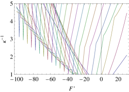
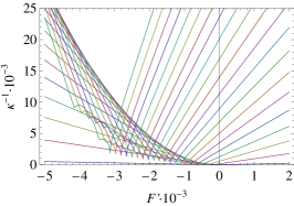
Figure 2: The dependence of convergence radius on $F^{\prime}$ for $G^{\prime}=5..705$ (top) and for $G^{\prime}=5..21000$ (bottom).

V Results

Detailed analysis of the solution was done in the earlier studies. Where the attention was centered on the case of large ${\rm Re}$. Our new finding deals with the case of small ${\rm Re}$ when the viscous term is comparable or larger than the convective one. This difference arises when new terms in the solution (20-III) dominate, i.e. when ${\rm Re}$ is small.

In the case of $F=0$ the result is shown in Fig. 3.

Figure 3: $\kappa=0.5$, ${\rm Re}=1$, $F=0$. Comparison of solutions. (a) $v_{\zeta}$, (b) $v_{\zeta}^{(c)}$, (c) $\psi$, (d) $\psi^{(c)}$.

One can see that the shift $\delta_{m}$ of the stream velocity maximum due to a centrifugal force directed outward from the torus axis is not valid at small Reynolds number. In fact for $\kappa\gtrsim 0.3$ there is a shift only in the opposite direction (inwards) because of viscous stresses in the region of convergence. This shift is mainly due to the difference (20). It has a dependence on ${\rm Re}$ shown in Fig. 4.

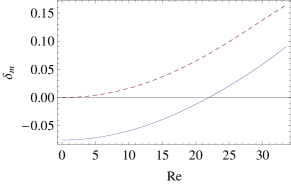
Figure 4: Shift $\delta_{m}$ of the maximum of stream velocity vs ${\rm Re}$ at $\kappa=0.1$. Dashed line stands corresponds to the solution $v_{\zeta}^{(c)}$.

When the torus rotates ($F\neq 0$) the Coriolis force gives rise to additional vortices in the cross-section. In the counter-rotating case such a vortex can act against the centrifugal vortex. This produces a four-vortex picture (see Fig. 5). Again we see that the flow pattern is different for a low Reynolds number. The vortex corresponding to the Coriolis force arises at the boundary while $\psi^{(c)}$ starts to grow in the center.

Figure 5: $\kappa=0.5$, ${\rm Re}=1$, $F=-0.63$. Comparison of solutions. (a) $\psi$, (b) $\psi^{(c)}$.

Axial shear-stress along the channel $\tau=-\left.\frac{\partial{v_{\zeta}}\mathstrut}{\partial{\rho}}\right|_{\rho=1}$ differs from that presented in Zhang et al. (2003). The first order residual is $3/16G\kappa\left(3\rho^{2}-1\right)\cos\varphi$. It does not change the pressure drop but produces a strong variation (about 40%) of friction at the boundary (see Fig. 6, thick curves). There is a similar difference in the azimuthal shear-stress $\tau_{\varphi}=-\left.\frac{\partial{v_{\varphi}}\mathstrut}{\partial{\rho}}\right|_{\rho=1}$. The second order residual is

$$\tau_{\varphi}-\tau_{\varphi}^{c}=\frac{G{\rm Re}(13G-25)\kappa^{2}\sin 2\varphi}{3840}.$$ (22)

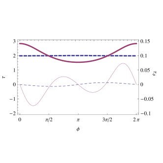
Figure 6: Axial shear-stress $\tau$ (bold lines, tick labels at left) and azimuthal shear-stress $\tau_{\varphi}$ (thin lines, tick labels at right) dependencies on angle: Dashed lines corresponds to the solution in Zhang et al. (2003). $\kappa=0.4,{{\rm Re}}=10,F=-0.49$.

This work shows that solution of the full governing equations reveals some specific features for flow in a toroidal channel: a shift of the maximum of the stream velocity toward the inner axis, the appearance of a second pair of vortices at the internal boundary, an additional $\varphi$-dependance of stresses. These are well pronounced at low values of the Reynolds number. The solution for a giving curvature $\kappa$ asymptotically approaches the known solution Zhang et al. (2003) at high ${\rm Re}$.