Spectral resolution in hyperbolic orbifolds, quantum chaos, and cosmology

Abstract

We present a few subjects from physics that have one in common: the spectral resolution of the Laplacian.

1 Introduction

If we look to nature, we observe dynamics and structure formation in various aspects. Several theories exist that explain the growth of structure quantitatively. On the smallest scale, it is quantum mechanics that governs the dynamics, whereas on the largest scale the evolution of our universe follows the Einstein field equations.

For all scales and almost any kind of observation we have equations at hand that quantify our findings. Many of these equations contain the spectral resolution of the Laplacian. Just think of the Schrödinger equation. In absence of forces or when the potential can be transformed into the metric, the stationary Schrödinger equation reduces to the eigenvalue equation of the Laplacian subject to some boundary conditions.

Spectral resolution has important consequences on many topics. Focusing on a few particular subjects, we start with an example from thermodynamics and demonstrate the importance of the spectral density. According to Weyl’s law, the spectral density in leading order does not depend on the shape of the boundaries. In consequence, the properties of thermodynamic systems are universal.

Less universal is the distribution of the eigenvalues. A central subject of quantum chaos is to classify the distribution of eigenvalues in dependence of whether the corresponding classical system is chaotic. In an explicit example, we compute the spectrum of the Laplacian numerically and confirm a conjecture of arithmetic quantum chaos.

Finally, we use the eigenvalues and eigenfunctions of the Laplacian to compute the temperature fluctuations in the cosmic microwave background.

2 Thermodynamics

The thermodynamic properties of an ideal gas can be deduced from the logarithm of the partition function,

$$\ln Z\equiv-\eta\sum_{\alpha}\ln(1-\eta z\mathrm{e}^{-\beta\varepsilon_{\alpha}}),$$

where $\alpha$ stands for the quantum numbers of a single particle with energy $\varepsilon_{\alpha}$, $z=\mathrm{e}^{\beta\mu}$ is the fugacity, $\beta=\frac{1}{kT}$ is the inverse temperature, and $\eta$ is the statistic parameter that distinguishes between bosons, $\eta=1$, and fermions, $\eta=-1$.

Introducing the spectral density

$$d(\varepsilon):=\sum_{\alpha}\delta(\varepsilon-\varepsilon_{\alpha})$$

the partition function can be expressed by an integral

$$\ln Z=-\eta\int_{-\infty}^{\infty}d(\varepsilon)\ln(1-\eta z\mathrm{e}^{-\beta\varepsilon})\,\mathrm{d}\varepsilon$$

with the advantage that it is easier to compute an integral than a sum analytically.

Example 1 (The ideal gas inside a cube)

The quantum microstate of an ideal gas in thermal equilibrium is subject to the stationary Schrödinger equation

$$H\Psi=E\Psi$$

with Dirichlet boundary conditions at $x,y,z=0$ and $x,y,z=L$. Since the Hilbert space of an ideal gas separates, the Hamiltonian $H$ can be expressed by the sum of single-particle Hamiltonians $h_{j}=-\frac{\hbar^{2}}{2m}\Delta_{j},\ j=1,\ldots,N$, where the Laplacian $\Delta_{j}$ acts only on the coordinates of the $j$-th particle. Solving $h\psi=\varepsilon\psi$ yields the single-particle wave functions

$$\psi_{n_{x},n_{y},n_{z}}=\sqrt{\tfrac{2}{L}}\sin\Big{(}\frac{p_{x}x}{\hbar}\Big{)}\sqrt{\tfrac{2}{L}}\sin\Big{(}\frac{p_{y}y}{\hbar}\Big{)}\sqrt{\tfrac{2}{L}}\sin\Big{(}\frac{p_{z}z}{\hbar}\Big{)}$$

and the single-particle eigenvalues

$$\varepsilon_{n_{x},n_{y},n_{z}}=\frac{p_{x}^{2}+p_{y}^{2}+p_{z}^{2}}{2m}=\frac{\hbar^{2}\pi^{2}}{2mL^{2}}(n_{x}^{2}+n_{y}^{2}+n_{z}^{2})$$

with the quantum numbers $n_{x},n_{y},n_{z}\in\mathds{N}$.

In the thermodynamic limit, $V\to\infty$, the spectrum becomes continuous. Consequently, the sum over the quantum numbers,

$$\sum_{\alpha}=\sum_{n_{x}}\sum_{n_{y}}\sum_{n_{z}}\sum_{m=-s}^{s},$$

can be replaced by integrals

$$\sum_{n_{x}=1}^{\infty}\to\int_{0}^{\infty}\mathrm{d}n_{x}=\frac{L}{2\pi\hbar}\int_{-\infty}^{\infty}\mathrm{d}p_{x}\,,\qquad\mathrm{d}p_{x}=\frac{\hbar\pi}{L}\mathrm{d}n_{x},$$

resulting in

$$\sum_{\alpha}\to\frac{V}{(2\pi\hbar)^{3}}(2s+1)\int_{\mathds{R}^{3}}\mathrm{d}^{3}p,$$

where $V=L^{3}$ is the volume and $s$ is the spin.

Evaluating the spectral density

$$d(\varepsilon)=\sum_{\alpha}\delta(\varepsilon-\varepsilon_{\alpha})\to\frac{V}{(2\pi\hbar)^{3}}(2s+1)\int\mathrm{d}^{3}p\,\delta(\varepsilon-\varepsilon_{\alpha})$$

with

$$\delta(\varepsilon-\varepsilon_{\alpha})=\delta(\varepsilon-\frac{p^{2}}{2m})=\frac{2m}{2|p|}\big{(}\delta(|p|-\sqrt{2m\varepsilon})+\delta(|p|+\sqrt{2m\varepsilon})\big{)}.$$

yields

$$d(\varepsilon)\sim(2s+1)\frac{(2m)^{\frac{3}{2}}}{4\pi^{2}\hbar^{3}}V\sqrt{\varepsilon}\quad\text{for}\quad\varepsilon\geq 0\qquad\text{and}\qquad d(\varepsilon)=0\quad\text{for}\quad\varepsilon<0.$$

Inserting it into the partition function gives

$$\ln Z=-\eta(2s+1)\frac{V}{\lambda^{3}}\frac{2}{\sqrt{\pi}}\int_{0}^{\infty}\mathrm{d}x\,\sqrt{x}\ln(1-\eta z\mathrm{e}^{-x})\,,\qquad\lambda:=\sqrt{\tfrac{2\pi\hbar^{2}}{m}\beta}\,.$$

Taylor expanding the integrand

$$\ln(1-\eta z\mathrm{e}^{-x})=-\sum_{n=1}^{\infty}\frac{(\eta z\mathrm{e}^{-x})^{n}}{n}=\eta z\mathrm{e}^{-x}+\frac{1}{2}z^{2}\mathrm{e}^{-2x}+O(z^{3}),$$

and evaluating the conditioning equation for the chemical potential, we have

$$N\equiv z\frac{\partial\ln Z}{\partial z}=(2s+1)\frac{V}{\lambda^{3}}z\big{(}1+\eta\frac{z}{2\sqrt{2}}+O(z^{2})\big{)}.$$

Hence, the thermal equation of state

$$J:=-\frac{1}{\beta}\ln Z\equiv-pV,$$

results in the virial expansion of the ideal gas

$$pV=NkT\big{(}1-\frac{\eta}{2s+1}\frac{N}{V}\frac{\lambda^{3}}{4\sqrt{2}}+\ldots\big{)}.$$

Interested in the inner energie, we obtain

$$U\equiv-\frac{\partial}{\partial\beta}\ln Z=\frac{3}{2}\frac{1}{\beta}\ln Z=\frac{3}{2}pV.$$

For further details and insight into thermodynamics, we refer the reader to any standard textbook on statistical physics, e.g. [15].

But what, if we ask for the ideal gas being inside a 3-sphere? Do we need to compute the entire example again, beginning with the spectral resolution of the Laplacian in a sphere?

Theorem 1 (Weyl’s law [29, 4])

If a quantum system is restricted to a finite volume $V$ in $D$ dimensions, its level counting function

$$N(E):=\#\{\,E_{i}\,|\,E_{i}\leq E\}\equiv\int_{-\infty}^{E}d(E)\,\mathrm{d}E$$

is asymptotically equal to

$$N(E)\sim(2s+1)C_{D}VE^{\frac{D}{2}}$$

in the semiclassical limit, $E\to\infty$, where

$$C_{D}=\frac{1}{\Gamma(\frac{D}{2}+1)}\big{(}\frac{m}{2\pi\hbar^{2}}\big{)}^{\frac{D}{2}}$$

is a universal constant that only depends on the dimension $D$, but not on the specific shape of the boundary.

Weyl’s law is nice. It tells us that the results of thermodynamics are universal, i.e. they are independent of the boundary shape.

3 Quantum chaos

In terms of classical mechanics a system is described by specifying the values of its coordinates and velocities, $x_{1},\ldots,x_{f}$ and $\dot{x}_{1},\ldots,\dot{x}_{f}$, where $f$ is the number of degrees of freedom.

If there exist $f$ linear independent constants of motion that are in involution with each other, there is a set of canonical coordinates on the phase space, the action-angle variables. The action variables are constants of motion and the angle variables are the natural linear, periodic coordinates on the torus. The motion on the torus is linear in the angle variables, and the system is called classically integrable.

If there do not exist $f$ linear independent constants of motion, the system is called classical non-integrable or chaotic. The dynamics is non-linear and shows an exponential sensitivity to initial conditions.

Being a limiting case of quantum mechanics, one might expect to see the properties of classical mechanics in quantum theory. But it is not this simple. The Schrödinger equation is linear and there is no exponential sensitivity to initial conditions. Quantum chaos relies on the behaviour of the corresponding classical system. A quantum system is called chaotic if and only if the corresponding classical system is non-integrable.

Central questions of quantum chaos concern the eigenvalue statistics and the distribution of eigenvalues in the semiclassical limit.

We use the following assumptions: The quantum mechanical system is desymmetrised with respect to all its unitary symmetries, and whenever we examine the distribution of the eigenvalues, we regard them on the scale of the mean level spacings. Moreover, it is believed that after desymmetrisation a generic quantum Hamiltonian possesses no degenerate eigenvalues.

Conjecture 1 (Berry, Tabor [6])

If the corresponding classical system is integrable, the eigenvalues behave like independent random variables and the distribution of the nearest-neighbour spacings is close to the Poisson distribution, i.e. there is no level repulsion.

Conjecture 2 (Bohigas, Giannoni, Schmit [8, 9])

If the corresponding classical system is chaotic, the eigenvalues are distributed like the eigenvalues of hermitian random matrices. The corresponding ensembles depend only on the symmetries of the system:

• For chaotic systems without time-reversal invariance the distribution of the eigenvalues should be close to the distribution of the Gaussian Unitary Ensemble (GUE) which is characterised by a quadratic level repulsion.

• For chaotic systems with time-reversal invariance and integer spin the distribution of the eigenvalues should be close to the distribution of the Gaussian Orthogonal Ensemble (GOE) which is characterised by a linear level repulsion.

• For chaotic systems with time-reversal invariance and half-integer spin the distribution of the eigenvalues should be close to the distribution of the Gaussian Symplectic Ensemble (GSE) which is characterised by a quartic level repulsion.

These conjectures are very well confirmed by numerical calculations, but several exceptions are known. Here are two examples:

Exception 1

The harmonic oscillator is classically integrable, but its spectrum is equidistant.

Exception 2

The geodesic motion on surfaces with constant negative curvature provides a prime example for classical chaos. In some cases, however, the nearest-neighbour distribution of the eigenvalues of the Laplacian on these surfaces appears to be Poissonian.

Conjecture 3 (Arithmetic Quantum Chaos [7, 10])

On surfaces of constant negative curvature that are generated by arithmetic fundamental groups, the distribution of the eigenvalues of the quantum Hamiltonian are close to the Poisson distribution. Due to level clustering small spacings occur comparably often.

In the next sections, we compute numerically the eigenvalues and eigenfunctions of the Laplacian that describe the quantum mechanics of a point particle moving freely in the non-integrable three-dimensional hyperbolic space of constant negative curvature generated by the Picard group. The Picard group is arithmetic and we find that our results are in accordance with the conjecture of arithmetic quantum chaos.

4 The modular surface

For simplicity we first introduce the topology and geometry of the two-dimensional surface of constant negative curvature that is generated by the modular group [26]. It will then be easy to carry over to the three-dimensional space of constant negative curvature that is generated by the Picard group.

The construction begins with the upper half-plane,

$${\cal H}=\{(x,y)\in\mathds{R}^{2},\quad y>0\},$$

equipped with the hyperbolic metric of constant negative curvature

$$ds^{2}=\frac{dx^{2}+dy^{2}}{y^{2}}.$$

A free particle on the upper half-plane moves along geodesics, which are straight lines and semicircles perpendicular to the $x$-axis, respectively. Expressing a point $(x,y)\in{\cal H}$ as a complex number $z=x+\mathrm{i}y$, all isometries of the hyperbolic metric are given by the group of linear fractional transformations,

$$z\mapsto\gamma z=\frac{az+b}{cz+d},\quad a,b,c,d\in\mathds{R},\quad ad-bc=1,$$

which is isomorphic to the group of matrices

$$\gamma=\begin{pmatrix}a&b\\ c&d\end{pmatrix}\in\operatorname{SL}(2,\mathds{R}),$$

up to a common sign of the matrix entries,

$$\operatorname{SL}(2,\mathds{R})/\{\pm 1\}=\operatorname{PSL}(2,\mathds{R}).$$

In analogy to the concept of a fundamental cell in a regular lattice of a crystal we can introduce a fundamental domain of a discrete group $\Gamma\subset\operatorname{PSL}(2,\mathds{R})$.

Definition 1

A fundamental domain of the discrete group $\Gamma$ is an open subset ${\cal F}\subset{\cal H}$ with the following conditions: The closure of ${\cal F}$ meets each orbit $\Gamma z=\{\gamma z,\ \gamma\in\Gamma\}$ at least once, ${\cal F}$ meets each orbit $\Gamma z$ at most once, and the boundary of ${\cal F}$ has Lebesgue measure zero.

If we choose the group $\Gamma$ to be the modular group,

$$\Gamma=\operatorname{PSL}(2,\mathds{Z}),$$

which is generated by a translation and an inversion,

$$\begin{pmatrix}1&1\\ 0&1\end{pmatrix}:\ z\mapsto z+1\qquad\text{and}\qquad\begin{pmatrix}0&-1\\ 1&0\end{pmatrix}:\ z\mapsto-z^{-1},$$

the fundamental domain of standard shape is

$${\cal F}=\{z=x+\mathrm{i}y\in{\cal H},\quad-\frac{1}{2}<x<\frac{1}{2},\quad|z|>1\}.$$

The isometric copies of the fundamental domain $\gamma{\cal F},\ \gamma\in\Gamma$, tessellate the upper half-plane completely without any overlap or gap. Identifying the fundamental domain ${\cal F}$ and parts of its boundary with all its isometric copies $\gamma{\cal F},\ \forall\gamma\in\Gamma$, defines the topology to be the quotient space $\Gamma\backslash{\cal H}$. The quotient space $\Gamma\backslash{\cal H}$ can also be thought of as the fundamental domain ${\cal F}$ with its faces glued according to the elements of the group $\Gamma$.

Any function being defined on the upper half-plane that is invariant under linear fractional transformations,

$$f(z)=f(\gamma z)\quad\forall\gamma\in\Gamma,$$

can be identified with a function living on the quotient space $\Gamma\backslash{\cal H}$ and vice versa.

With the hyperbolic metric the quotient space $\Gamma\backslash{\cal H}$ inherits the structure of an orbifold. An orbifold locally looks like a manifold, with the exception that it is allowed to have elliptic fixed-points.

The orbifold of the modular group has one parabolic and two elliptic fixed-points,

$$z=\mathrm{i}\infty,\quad z=\mathrm{i},\quad\text{and}\quad z=\frac{1}{2}+\mathrm{i}\frac{\sqrt{3}}{2}.$$

The parabolic one fixes a cusp at $z=\mathrm{i}\infty$ which is invariant under the parabolic element

$$\begin{pmatrix}1&1\\ 0&1\end{pmatrix}.$$

Hence, the orbifold of the modular group is non-compact. The volume element corresponding to the hyperbolic metric reads

$$d\mu=\frac{dxdy}{y^{2}},$$

such that the volume of the orbifold $\Gamma\backslash{\cal H}$ is finite,

$$\operatorname{vol}(\Gamma\backslash{\cal H})=\frac{\pi}{3}.$$

Scaling the units such that $\hbar=1$ and $2m=1$, the stationary Schrödinger equation which describes the quantum mechanics of a point particle moving freely in the orbifold $\Gamma\backslash{\cal H}$ becomes

$$(\Delta+\lambda)f(z)=0,$$

where the hyperbolic Laplacian is given by

$$\Delta=y^{2}(\frac{\partial^{2}}{\partial x^{2}}+\frac{\partial^{2}}{\partial y^{2}})$$

and $\lambda$ is the scaled energy. We can relate the eigenvalue problem defined on the orbifold $\Gamma\backslash{\cal H}$ to the eigenvalue problem defined on the upper-half space, with the eigenfunctions being subject to the automorphy condition relative to the discrete group $\Gamma$,

$$f(\gamma z)=f(z)\quad\forall\gamma\in\Gamma.$$

In order to avoid solutions that grow exponentially in the cusp, we impose the boundary condition

$$f(z)=O(y^{\kappa})\quad\text{for}\quad z\to\mathrm{i}\infty,$$

where $\kappa$ is some positive constant.

The solutions of this eigenvalue problem can be identified with Maass waveforms [17]. Numerically, they are most efficiently computed using Hejhal’s algorithm [14].

5 The Picard surface

In the three-dimensional case one considers the upper-half space,

$${\cal H}=\{(x_{0},x_{1},y)\in\mathds{R}^{3},\quad y>0\}$$

equipped with the hyperbolic metric

$$ds^{2}=\frac{dx_{0}^{2}+dx_{1}^{2}+dy^{2}}{y^{2}}.$$

The geodesics of a particle moving freely in the upper half-space are straight lines and semicircles perpendicular to the $x_{0}$-$x_{1}$-plane, respectively.

Expressing any point $(x_{0},x_{1},y)\in{\cal H}$ as a quaternion, $z=x_{0}+\mathrm{i}x_{1}+\mathrm{j}y$, with the multiplication defined by $\mathrm{i}^{2}=-1,\ \mathrm{j}^{2}=-1,\ \mathrm{i}\mathrm{j}+\mathrm{j}\mathrm{i}=0$, all motions in the upper half-space are given by linear fractional transformations

$$z\mapsto\gamma z=(az+b)(cz+d)^{-1},\quad a,b,c,d\in\mathds{C},\quad ad-bc=1.$$

The group of these transformations is isomorphic to the group of matrices

$$\gamma=\begin{pmatrix}a&b\\ c&d\end{pmatrix}\in\operatorname{SL}(2,\mathds{C})$$

up to a common sign of the matrix entries,

$$\operatorname{SL}(2,\mathds{C})/\{\pm 1\}=\operatorname{PSL}(2,\mathds{C}).$$

The motions provided by the elements of $\operatorname{PSL}(2,\mathds{C})$ exhaust all orientation preserving isometries of the hyperbolic metric on ${\cal H}$.

We now choose the discrete group $\Gamma\subset\operatorname{PSL}(2,\mathds{C})$ that is generated by the cosets of the following elements,

$$\begin{pmatrix}1&1\\ 0&1\end{pmatrix},\quad\begin{pmatrix}1&\mathrm{i}\\ 0&1\end{pmatrix},\quad\begin{pmatrix}0&-1\\ 1&0\end{pmatrix},$$

which yield two translations and one inversion,

$$z\mapsto z+1,\quad z\mapsto z+\mathrm{i},\quad z\mapsto-z^{-1}.$$

This group $\Gamma$ is called the Picard group. The three motions generating $\Gamma$, together with the coset of the element

$$\begin{pmatrix}\mathrm{i}&0\\ 0&-\mathrm{i}\end{pmatrix}$$

that is isomorphic to the symmetry

$$z=x+\mathrm{j}y\mapsto\mathrm{i}z\mathrm{i}=-x+\mathrm{j}y,$$

can be used to construct the fundamental domain of standard shape

$${\cal F}=\{z=x_{0}+\mathrm{i}x_{1}+\mathrm{j}y\in{\cal H},\quad-\frac{1}{2}<x_{0}<\frac{1}{2},\quad 0<x_{1}<\frac{1}{2},\quad|z|>1\}.$$

Identifying the faces of the fundamental domain according to the elements of the group $\Gamma$ leads to a realisation of the quotient space $\Gamma\backslash{\cal H}$.

With the hyperbolic metric the quotient space $\Gamma\backslash{\cal H}$ inherits the structure of an orbifold that has one parabolic and four elliptic fixed-points,

$$z=\mathrm{j}\infty,\quad z=\mathrm{j},\quad z=\frac{1}{2}+\mathrm{j}\sqrt{\frac{3}{4}},\quad z=\frac{1}{2}+\mathrm{i}\frac{1}{2}+\mathrm{j}\sqrt{\frac{1}{2}},\quad z=\mathrm{i}\frac{1}{2}+\mathrm{j}\sqrt{\frac{3}{4}}.$$

The parabolic fixed-point corresponds to a cusp at $z=\mathrm{j}\infty$ that is invariant under the parabolic elements

$$\begin{pmatrix}1&1\\ 0&1\end{pmatrix}\quad\text{and}\quad\begin{pmatrix}1&\mathrm{i}\\ 0&1\end{pmatrix}.$$

The volume element deriving from the hyperbolic metric reads

$$d\mu=\frac{dx_{0}dx_{1}dy}{y^{3}},$$

such that the volume of the non-compact orbifold $\Gamma\backslash{\cal H}$ is finite,

$$\operatorname{vol}(\Gamma\backslash{\cal H})=\frac{\zeta_{K}(2)}{4\pi^{2}}\simeq 0.3053218647...,$$

where

$$\zeta_{K}(s)=\frac{1}{4}\sum_{\nu\in\mathds{Z}[\mathrm{i}]-\{0\}}(\nu\bar{\nu})^{-s},\quad\Re s>1,$$

is the Dedekind zeta function.

We are interested in the square-integrable eigenfunctions of the Laplacian,

$$\Delta=y^{2}\big{(}\frac{\partial^{2}}{\partial x_{0}^{2}}+\frac{\partial^{2}}{\partial x_{1}^{2}}+\frac{\partial^{2}}{\partial y^{2}}\big{)}-y\frac{\partial}{\partial y},$$

that determine the quantum mechanics of a point particle moving freely in the orbifold $\Gamma\backslash{\cal H}$. We identify the solutions with Maass waveforms [18].

Since Maass waveforms are automorphic, and therefore periodic in $x_{0}$ and $x_{1}$, it follows that they can be expanded into a Fourier series,

$$f(z)=u(y)+\sum_{\beta\in\mathds{Z}[\mathrm{i}]-\{0\}}a_{\beta}yK_{\mathrm{i}r}(2\pi|\beta|y)\operatorname{e}^{2\pi\mathrm{i}\Re\beta x},$$

where

$$u(y)=\begin{cases}b_{0}y^{1+\mathrm{i}r}+b_{1}y^{1-\mathrm{i}r}&\text{if $r\not=0$},\\ b_{2}y+b_{3}y\ln y&\text{if $r=0$}.\end{cases}$$

$K_{\mathrm{i}r}(x)$ is the K-Bessel function whose order is connected with the eigenvalue $\lambda$ by

$$\lambda=r^{2}+1.$$

If a Maass waveform vanishes in the cusp,

$$\lim_{z\to\mathrm{j}\infty}f(z)=0,$$

it is called a Maass cusp form. Maass cusp forms are square integrable over the fundamental domain, $\langle f,f\rangle<\infty$, where

$$\langle f,g\rangle=\int_{\Gamma\backslash{\cal H}}\bar{f}g\,d\mu$$

is the Petersson scalar product.

According to the Roelcke-Selberg spectral resolution of the Laplacian [22], its spectrum contains both a discrete and a continuous part. The discrete part is spanned by the constant eigenfunction $f_{0}$ and a countable number of Maass cusp forms $f_{1},f_{2},f_{3},\ldots$ which we take to be ordered with increasing eigenvalues, $0=\lambda_{0}<\lambda_{1}\leq\lambda_{2}\leq\lambda_{3}\leq\ldots$. The continuous part of the spectrum $\lambda\geq 1$ is spanned by the Eisenstein series $E(z,1+\mathrm{i}r)$ which are known analytically [11]. The Fourier coefficients of the functions $\Lambda_{K}(1+\mathrm{i}r)E(z,1+\mathrm{i}r)$ are given by

$$b_{0}=\Lambda_{K}(1+\mathrm{i}r),\quad b_{1}=\Lambda_{K}(1-\mathrm{i}r),\quad a_{\beta}=2\sum_{\begin{subarray}{c}\lambda,\mu\in\mathds{Z}[\mathrm{i}]\\ \lambda\mu=\beta\end{subarray}}\big{|}\frac{\lambda}{\mu}\big{|}^{\mathrm{i}r},$$

where

$$\Lambda_{K}(s)=4\pi^{-s}\Gamma(s)\zeta_{K}(s)$$

has an analytic continuation into the complex plane except for a pole at $s=1$.

Normalising the Maass cusp forms according to

$$\langle f_{n},f_{n}\rangle=1,$$

we can expand any square integrable function $\phi\in L^{2}(\Gamma\backslash{\cal H})$ in terms of Maass waveforms,

$$\phi(z)=\sum_{n\geq 0}\langle f_{n},\phi\rangle f_{n}(z)+\frac{1}{2\pi\mathrm{i}}\int_{\Re s=1}\langle E(\cdot,s),\phi\rangle E(z,s)\,ds.$$

The eigenvalues and their associated Maass cusp forms are not known analytically. Thus, one has to approximate them numerically. By making use of the Hecke operators and the multiplicative relations among the coefficients, Steil [25] obtained a non-linear system of equations which allowed him to compute $2545$ consecutive eigenvalues. In [28], we extend these computations with the use of a variant of Hejhal’s algorithm [14]. Our favourite explanation of the algorithm is published in [27].

6 Results

The modular surface, i.e. the two-dimensional hyperbolic orbifold that is generated by the modular group, has a reflection symmetry. This reflection symmetry commutes with the Laplacian. Consequently, the eigenfunctions fall into two symmetry classes. We call an eigenfunction to be even or odd depending on whether $f(-x+\mathrm{i}y)=f(x+\mathrm{i}y)$ or $f(-x+\mathrm{i}y)=-f(x+\mathrm{i}y)$ holds. We also call the corresponding eigenvalue to be even or odd, respectively.

In table 1, the first ten consecutive even and the first ten consecutive odd eigenvalues of the Laplacian on the modular surface are listed.

Table 1: The first ten even and the first ten odd eigenvalues of the negative Laplacian on the modular surface. Listed is $r$, related to the eigenvalue via $\lambda=r^{2}+\frac{1}{4}$.

even odd

$$13 .77975135189 9 .53369526135$$

$$17 .73856338106 12 .17300832468$$

$$19 .42348147083 14 .35850951826$$

$$21 .31579594020 16 .13807317152$$

$$22 .78590849419 16 .64425920190$$

$$24 .11235272984 18 .18091783453$$

$$25 .82624371271 19 .48471385474$$

$$26 .15208544922 20 .10669468255$$

$$27 .33270808315 21 .47905754475$$

$$28 .53074769292 22 .19467397757$$

Table 2: The first few eigenvalues of the negative Laplacian on the Picard surface. Listed is $r$, related to the eigenvalues via $\lambda=r^{2}+1$.

$${\mathbf{D}} {\mathbf{G}} {\mathbf{C}} {\mathbf{H}}$$

$$\ 8 .55525104 \ 6 .62211934$$

$$11 .10856737 10 .18079978$$

$$12 .86991062 12 .11527484 12 .11527484$$

$$14 .07966049 12 .87936900$$

$$15 .34827764 14 .14833073$$

$$15 .89184204 14 .95244267 14 .95244267$$

$$17 .33640443 16 .20759420$$

$$17 .45131992 17 .45131992 16 .99496892 16 .99496892$$

$$17 .77664065 17 .86305643 17 .86305643$$

$$19 .06739052 18 .24391070$$

$$19 .22290266 18 .83298996$$

$$19 .41119126 19 .43054310 19 .43054310$$

$$20 .00754583 20 .30030720 20 .30030720$$

$$20 .70798880 20 .70798880 20 .60686743$$

$$20 .81526852 21 .37966055 21 .37966055$$

$$21 .42887079 21 .44245892$$

$$22 .12230276 21 .83248972 21 .83248972$$

$$22 .63055256 22 .58475297 22 .58475297$$

$$22 .96230105 22 .96230105 22 .85429195$$

$$23 .49617692 23 .49768305 23 .49768305$$

The Picard surface, i.e. the three-dimensional hyperbolic orbifold that is generated by the Picard group, has two symmetries such that the eigenfunctions of the Laplacian fall into four symmetry classes. The eigenfunctions and their corresponding eigenvalues are called to be of symmetry class ${\mathbf{D}}$, ${\mathbf{G}}$, ${\mathbf{C}}$, or ${\mathbf{H}}$ depending on whether

$$f(x+\mathrm{j}y)=f(\mathrm{i}x+\mathrm{j})=f(-\bar{x}+\mathrm{j}y),$$

$$f(x+\mathrm{j}y)=f(\mathrm{i}x+\mathrm{j})=-f(-\bar{x}+\mathrm{j}y),$$

$$f(x+\mathrm{j}y)=-f(\mathrm{i}x+\mathrm{j})=f(-\bar{x}+\mathrm{j}y),$$

$$f(x+\mathrm{j}y)=-f(\mathrm{i}x+\mathrm{j})=-f(-\bar{x}+\mathrm{j}y)$$

holds, respectively.

The first few consecutive eigenvalues of each symmetry class of the Laplacian on the Picard surface are listed in table 2.

Examining the eigenvalues, we find that there occur degenerate eigenvalues. The smallest degenerate eigenvalue of the Laplacian on the Picard surface is $\lambda=12.11527484^{2}+1$. The degeneracies result from the symmetries of the Picard surface. If desymmetrised, i.e. within a given symmetry class, there do not exist any degenerate eigenvalues. An explanation is given in [28].

Consider the level counting function

$$N(r):=\#\{\,r_{i}\ |\ r_{i}\leq r\}$$

and split it into two parts

$$N(r)=\bar{N}(r)+N_{fluc}(r).$$

Here $\bar{N}$ is a smooth function describing the average increase in the number of levels and $N_{fluc}$ describes the fluctuations around the mean such that

$$\lim_{R\to\infty}\frac{1}{R}\int_{1}^{R}N_{fluc}(r)dr=0.$$

According to Weyl’s law and higher order corrections for the Picard surface found by Matthies [19], the average increase in the number of levels is given by

$$\bar{N}(r)=\tfrac{\operatorname{vol}({\cal F})}{6\pi^{2}}r^{3}+a_{2}r\log r+a_{3}r+a_{4}$$

with the constants

$$a_{2} =-\tfrac{3}{2\pi},$$

$$a_{3} =\tfrac{1}{\pi}[\tfrac{13}{16}\log 2+\tfrac{7}{4}\log\pi-\log\Gamma(\tfrac{1}{4})+\tfrac{2}{9}\log(2+\sqrt{3})+\tfrac{3}{2}],$$

$$a_{4} =-\tfrac{1}{2}.$$

If desymmetrised into the four symmetry classes, the average increase in the number of levels is given by

$$\bar{N}(r)=\tfrac{1}{4}\tfrac{\operatorname{vol}({\cal F})}{6\pi^{2}}r^{3}+b_{1}r^{2}+b_{2}r\log r+b_{3}r+b_{4}$$

with the constants depending on the symmetry class as listed in table 3.

Table 3: The constants for the higher order corrections to Weyl’s law for each of the four symmetry classes of the Picard surface. The constants $b_{1}$ and $b_{2}$ are known analytically [19], whereas the constants $b_{3}$ and $b_{4}$ have been approximated numerically [28].

$$b_{1} b_{2} b_{3}\ \qquad b_{4}\qquad$$

$${\mathbf{D}} \tfrac{1}{24} -\tfrac{13}{8\pi} 0.8639... -0.288...$$

$${\mathbf{G}} -\tfrac{1}{24} \tfrac{3}{8\pi} 0.0285... -0.184...$$

$${\mathbf{C}} \tfrac{1}{96} -\tfrac{1}{8\pi} 0.0150... -0.062...$$

$${\mathbf{H}} -\tfrac{1}{96} -\tfrac{1}{8\pi} 0.0702... 0.034...$$

Figure 1: Level spacing distributions for the symmetry classes ${\mathbf{D}}$ (top left), ${\mathbf{G}}$ (top right), ${\mathbf{C}}$ (bottom left), and ${\mathbf{H}}$ (bottom right) of the Picard surface. The abscissae display the spacings $s$. The small crosses are the histograms of altogether $13949$ nearest-neighbour spacings. The dashed curves starting at the origins are the integrated distributions. For comparison, the full curves show the Poisson distribution.

Unfolding the spectrum,

$$x_{i}:=\bar{N}(r_{i}),$$

we are able to examine the distribution of the eigenvalues on the scale of the mean level spacings. Defining the sequence of nearest-neighbour level spacings with mean value $1$ as $i\to\infty$,

$$s_{i}:=x_{i+1}-x_{i},$$

we find that the spacing distribution comes close to that of a Poisson random process,

$$P_{\text{Poisson}}(s)=\mathrm{e}^{-s},$$

see figure 1, in accordance with the conjecture of arithmetic quantum chaos.

7 Cosmology

In the remaining sections we apply the eigenvalues and eigenfunctions of the Laplacian to a perturbed Robertson-Walker universe and compute the temperature fluctuations in the cosmic microwave background (CMB).

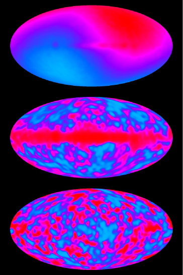
Figure 2: Sky maps of the temperature fluctuations in the CMB as observed by the NASA satellite mission COBE. The sky map on the top shows the dipole anisotropy after the mean background temperature of $T_{0}=2.725\,\text{K}$ has been subtracted. The amplitude of the dipole anisotropy is about $3\,\text{mK}$. Also subtracting the dipole yields the sky map in the middle. One sees the small temperature fluctuations whose amplitude is roughly $30\,\mu\text{K}$. But one also sees a lot of foreground contamination along the equator that comes from nearby stars in our galaxy. After removing the foregrounds one finally gets the sky map on the bottom showing the temperature fluctuations in the CMB. Downloaded from [30].

Figure 3: The expanding universe. At the time of last scattering occured a phase transition from an opaque to a transparent universe.

The CMB is a relic from the primeval fireball of the early universe. It is the light that comes from the time when the universe was $379\,000$ years old. It was predicted by Gamow in 1948 and explained in detail by Peebles [21]. In 1978, Penzias and Wilson won the Nobel Prize of Physics for first measuring the CMB at a wavelength of $7.35\,\text{cm}$. Within the resolution of their experiment they found the CMB to be completely isotropic over the whole sky. Later with the much better resolution of the NASA satellite mission Cosmic Background Explorer (COBE), Smoot et al. [23] found fluctuations in the CMB which are of amplitude $10^{-5}$ relative to the mean background temperature of $T_{0}=2.725\,\text{K}$, except for the large dipole moment, see figure 2, resulting in the Nobel Prize for Mather and Smoot in 2006. The small fluctuations in the CMB serve as a fingerprint of the early universe, since the temperature fluctuations are related to the density fluctuations at the time of last scattering. They show how isotropic the universe was at early times. In the inflationary scenario the fluctuations originate from quantum fluctuations which are inflated to macroscopic scales. Due to gravitational instabilities the fluctuations grow steadily and give rise to the formation of stars and galaxies.

The theoretical framework in which the CMB and its fluctuations are explained is Einstein’s general theory of relativity. Thereby a homogeneous and isotropic background given by a Robertson-Walker universe [12, 13, 16] is perturbed. The time-evolution of the perturbations can be computed in the framework of linear perturbation theory [5].

An explanation for the presence of the CMB is the following, see also figure 3: We live in an expanding universe. At early enough times the universe was so hot and dense that it was filled with a hot plasma consisting of ionised atoms, unbounded electrons, and photons. Due to Thomson scattering of photons with electrons, the hot plasma was in thermal equilibrium and the mean free path of the photons was small, hence the universe was opaque. Due to its expansion the universe cooled down and became less dense. When the universe was around $379\,000$ years old, its temperature $T$ has dropped down to approximately $3000\,\text{K}$. At this time, called the time of last scattering, the electrons got bound to the nuclei forming a gas of neutral atoms, mainly hydrogen and helium, and the universe became transparent. Since this time the photons travel freely on their geodesics through the universe. At the time of last scattering the photons had an energy distribution according to a Planck spectrum with temperature of nearly $3000\,\text{K}$. The further expansion of the universe redshifted the photons such that they nowadays have an energy distribution according to a Planck spectrum with temperature of $T_{0}=2.725\,\text{K}$. This is what we observe as the CMB.

Due to the thermal equilibrium before the time of last scattering the CMB is nearly perfectly isotropic, but small density fluctuations lead to small temperature fluctuations. The reason for the small temperature fluctuations comes from a variety of effects. The most dominant effects are the gravitational redshift that is larger in the directions of overdense regions, a small time delay in the transition from opaque to transparent that slightly reduces the Hubble redshift in the directions of overdense regions, the intrinsic temperature fluctuations, and the Doppler effect due to the velocity of the plasma.

8 Robertson-Walker universes

Assuming a universe whose spatial part is locally homogeneous and isotropic, its metric is given by the Robertson-Walker metric,

$$ds^{2}=dt^{2}-\tilde{a}^{2}(t)\gamma_{ij}dx^{i}dx^{j},$$

where we use the Einstein summation convention. Notice that we have changed the notation. Instead of the quaternion $z$ for the spatial variables, we now write $x=x_{0}+\mathrm{i}x_{1}+\mathrm{j}x_{2}$. $\gamma_{ij}$ is the metric of a homogeneous and isotropic three-dimensional space, and the units are rescaled such that the speed of light is $c=1$. Introducing the conformal time $d\eta=\frac{dt}{\tilde{a}(t)}$ we have

$$ds^{2}=a^{2}(\eta)\big{[}d\eta^{2}-\gamma_{ij}dx^{i}dx^{j}\big{]},$$

where $a(\eta)=\tilde{a}(t(\eta))$ is the cosmic scale factor.

With the Robertson-Walker metric the Einstein equations simplify to the Friedmann equations [12, 13, 16]. One of the two Friedmann equations reads

$$a^{\prime 2}+\kappa a^{2}=\frac{8\pi G}{3}T_{0}^{0}a^{4}+\frac{1}{3}\Lambda a^{4}$$

and the other Friedmann equation is equivalent to local energy conservation. $a^{\prime}$ is the derivative of the cosmic scale factor with respect to the conformal time $\eta$. $\kappa$ is the curvature parameter which we choose to be negative, $\kappa=-1$. $G$ is Newton’s gravitational constant, $T^{\mu}_{\nu}$ is the energy-momentum tensor, and $\Lambda$ is the cosmological constant.

Assuming the energy and matter in the universe to be a perfect fluid consisting of radiation, non-relativistic matter, and a cosmological constant, the time-time component of the energy-momentum tensor reads

$$T^{0}_{0}=\varepsilon_{\text{r}}(\eta)+\varepsilon_{\text{m}}(\eta),$$

where the energy densities of radiation and matter scale like

$$\varepsilon_{\text{r}}(\eta)=\varepsilon_{\text{r}}(\eta_{0})\big{(}\frac{a(\eta_{0})}{a(\eta)}\big{)}^{4}\quad\text{and}\quad\varepsilon_{\text{m}}(\eta)=\varepsilon_{\text{m}}(\eta_{0})\big{(}\frac{a(\eta_{0})}{a(\eta)}\big{)}^{3}.$$

Here $\eta_{0}$ denotes the conformal time at the present epoch.

Specifying the initial conditions (Big Bang!) $a(0)=0,\ a^{\prime}(0)>0$, the Friedmann equation can be solved analytically [3],

$$a(\eta)=\frac{-\big{(}\frac{\Omega_{\text{r}}}{\Omega_{\text{c}}}\big{)}^{\frac{1}{2}}{\cal P}^{\prime}(\eta)+\frac{1}{2}\big{(}\frac{\Omega_{\text{m}}}{\Omega_{\text{c}}}\big{)}\big{(}{\cal P}(\eta)-\frac{1}{12}\big{)}}{2\big{(}{\cal P}(\eta)-\frac{1}{12}\big{)}^{2}-\frac{1}{2}\frac{\Omega_{\Lambda}\Omega_{\text{r}}}{\Omega_{\text{c}}^{2}}}a(\eta_{0}),$$

where ${\cal P}(\eta)\equiv{\cal P}(\eta;g_{2},g_{3})$ denotes the Weierstrass ${\cal P}$-function. The so-called invariants $g_{2}$ and $g_{3}$ are determined by the cosmological parameters,

$$g_{2}=\frac{\Omega_{\Lambda}\Omega_{\text{r}}}{\Omega_{\text{c}}^{2}}+\frac{1}{12},\quad g_{3}=\frac{1}{6}\frac{\Omega_{\Lambda}\Omega_{\text{r}}}{\Omega_{\text{c}}^{2}}-\frac{1}{16}\frac{\Omega_{\Lambda}\Omega_{\text{m}}^{2}}{\Omega_{\text{c}}^{3}}-\frac{1}{216},$$

with

$$\Omega_{\text{r}}=\frac{8\pi G\varepsilon_{\text{r}}(\eta_{0})}{3H^{2}(\eta_{0})},\quad\Omega_{\text{m}}=\frac{8\pi G\varepsilon_{\text{m}}(\eta_{0})}{3H^{2}(\eta_{0})},\quad\Omega_{\text{c}}=\frac{1}{H^{2}(\eta_{0})a^{2}(\eta_{0})},\quad\Omega_{\Lambda}=\frac{\Lambda}{3H^{2}(\eta_{0})},$$

where

$$H(\eta)=\frac{a^{\prime}(\eta)}{a^{2}(\eta)}$$

is the Hubble parameter.

9 Perturbed Robertson-Walker universes

The idealisation to an exact homogeneous and isotropic universe was essential to derive the spacetime of the Robertson-Walker universe. But obviously, we do not live in a universe that is perfectly homogeneous and isotropic. We see individual stars, galaxies, and in between large empty space. Knowing the spacetime of the Robertson-Walker universe, we can study small perturbations around the homogeneous and isotropic background. Since the amplitude of the large scale fluctuations in the universe is of relative size $10^{-5}$, we can use linear perturbation theory. In longitudinal gauge the most general scalar perturbation of the Robertson-Walker metric reads

$$ds^{2}=a^{2}(\eta)\big{[}(1+2\Phi)d\eta^{2}-(1-2\Psi)\gamma_{ij}dx^{i}dx^{j}\big{]},$$

where $\Phi=\Phi(\eta,x)$ and $\Psi=\Psi(\eta,x)$ are functions of spacetime.

Assuming that the energy and matter density in the universe can be described by a perfect fluid, consisting of radiation, non-relativistic matter, and a cosmological constant, and neglecting possible entropy perturbations, the Einstein equations reduce in first order perturbation theory [20] to

$$\Phi=\Psi,$$

$$\Phi^{\prime\prime}+3\hat{H}(1+c_{\text{s}}^{2})\Phi^{\prime}-c_{\text{s}}^{2}\Delta\Phi+\big{(}2\hat{H}^{\prime}+(1+3c_{\text{s}}^{2})(\hat{H}^{2}+1)\big{)}\Phi=0,$$

where $\hat{H}=\frac{a^{\prime}}{a}$ and $c_{\text{s}}^{2}=(3+\frac{9}{4}\frac{\varepsilon_{\text{m}}}{\varepsilon_{\text{r}}})^{-1}$ are given by the solution of the non-perturbed Robertson-Walker universe. In the partial differential equation for $\Phi$ the Laplacian occurs. If the initial and the boundary conditions of $\Phi$ are specified, the time-evolution of the metric perturbations can be computed.

With the separation ansatz

$$\Phi(\eta,x)=\sum_{k}f_{k}(\eta)\psi_{k}(x)+\int dk\,f_{k}(\eta)\psi_{k}(x),$$

where the $\psi_{k}$ are the eigenfunctions of the negative Laplacian, and the $E_{k}$ are the corresponding eigenvalues,

$$-\Delta\psi_{k}(x)=E_{k}\psi_{k}(x),$$

the partial differential equation for $\Phi$ simplifies to

$$f_{k}^{\prime\prime}(\eta)+3\hat{H}(1+c_{\text{s}}^{2})f_{k}^{\prime}(\eta)+\big{(}c_{\text{s}}^{2}E_{k}+2\hat{H}^{\prime}+(1+3c_{\text{s}}^{2})(\hat{H}^{2}+1)\big{)}f_{k}(\eta)=0.$$

These ordinary differential equations (one for each eigenvalue $E_{k}$) can be computed numerically in a straightforward way, and we finally obtain the metric of the whole universe. This gives the input to the Sachs-Wolfe formula which connects the metric perturbations with the temperature fluctuations,

$$\frac{\delta T}{T_{0}}(\hat{n})=2\Phi(\eta_{\text{SLS}},x(\eta_{\text{SLS}}))-\frac{3}{2}\Phi(0,x(0))+2\int_{\eta_{\text{SLS}}}^{\eta_{0}}d\eta\,\frac{\partial}{\partial\eta}\Phi(\eta,x(\eta)),$$

where $\hat{n}$ is a unit vector in the direction of the observed photons. $x(\eta)$ is the geodesic along which the light travels from the surface of last scattering (SLS) towards us, and $\eta_{\text{SLS}}$ is the time of last scattering.

If we choose the topology of the universe to be the Picard surface, we can use the Maass waveforms of sections 5 and 6 in the separation ansatz for the metric perturbations $\Phi$. Let us further choose the initial conditions to be

$$f_{k}(0)=\frac{\sigma_{k}\alpha}{\sqrt{E_{k}\sqrt{E_{k}-1}}}\quad\text{and}\quad f_{k}^{\prime}(0)=\frac{-\Omega_{\text{m}}f_{k}(0)}{16(\Omega_{\text{c}}\Omega_{\text{r}})^{\frac{1}{2}}},$$

[3], which carry over to a Harrison-Zel’dovich spectrum. $\alpha$ is a constant independent of $k$ which is fitted to the amplitude of the observed temperature fluctuations. The quantities $\sigma_{k}$ are normal distributed random numbers.

The following cosmological parameters are used $\Omega_{\text{m}}=0.3,\Omega_{\Lambda}=0.65,\Omega_{\text{c}}=1-\Omega_{\text{tot}}=1-\Omega_{\text{r}}-\Omega_{\text{m}}-\Omega_{\Lambda},H(\eta_{0})=100\,h_{0}\,\text{km}\,\text{s}^{-1}\,\text{Mpc}^{-1}$ with $h_{0}=0.65$. The density $\Omega_{\text{r}}\approx 10^{-4}$ is determined by the current temperature $T_{0}=2.725\,\text{K}$. The point of the observer is chosen to be at $x_{\text{obs}}=0.2+0.1\mathrm{i}+1.6\mathrm{j}$. For numerical reasons the infinite spectrum is cut such that only the discrete eigenvalues with $E_{k}=k^{2}+1\leq 19601$ and their corresponding eigenfunctions are taken into account. The necessary computations are carried out in [1]. The resulting sky map is shown in figure 4.

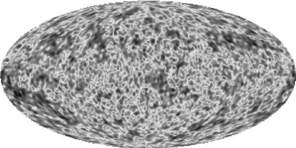
Figure 4: The sky map of the calculated temperature fluctuations of the CMB for $\Omega_{\text{tot}}=0.95,\Omega_{\text{m}}=0.3,\Omega_{\Lambda}=0.65,h_{0}=0.65$, and $x_{\text{obs}}=0.2+0.1\mathrm{i}+1.6\mathrm{j}$, if the discrete spectrum with $E_{k}=k^{2}+1\leq 19601$ is taken into account. (The figure is taken from [1]).

Concerning the topology of the universe which manifests itself in the suppression of power in the large scale anisotropies, there exist the cosmological observations from COBE and WMAP. In order to quantitatively compare our results with these observations, we introduce the two-point correlation function,

$$C(\vartheta)=\big{\langle}\delta T(\hat{n})\delta T(\hat{n}^{\prime})\big{\rangle}_{\cos\vartheta=\hat{n}\cdot\hat{n}^{\prime}}.$$

Figure 5 shows the correlation function corresponding to the calculated sky map of the Picard surface [2] in comparison with the results of the cosmological observations [24] and with the concordance model [24].

$C(\vartheta)\ [\mu\text{K}^{2}]$                                                 
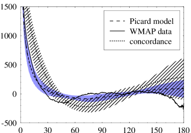
$\vartheta$

Figure 5: Correlation functions of the calculated temperature fluctuations on the Picard surface (dashed line) [2], of the WMAP observations (solid line) [24], and of the concordance model (dotted line) [24]. (The figure is borrowed from [2]).

We find quite good agreement of our calculated temperature fluctuations with the cosmological observations, whereas the results of the concordance model is not in good agreement with the data for $\vartheta\gtrsim 7^{\circ}$. Especially for large angular separations, $\vartheta\gtrsim 160^{\circ}$, the concordance model is not able to describe the observed anticorrelation in $C(\vartheta)$. This anticorrelation constitutes a fingerprint in the CMB that favours a non-trivial topology for the universe.

10 Acknowledgments

The author thanks Professor Hishamuddin Zainuddin for the invitation to the Theoretical Studies Laboratory at the Universiti Putra Malaysia and for the pleasant stay there. Collaborations with Ralf Aurich, Sven Lustig, and Frank Steiner are gratefully acknowledged. Highest thanks are due to Dennis A. Hejhal for sharing his knowledge with me. Part of the work has been supported by the European Commission under the Research Training Network (Mathematical Aspects of Quantum Chaos) no HPRN-CT-2000-00103. The free access to the Legacy Archive for Microwave Background Data Analysis (LAMBDA) [30] is appreciated. Support for LAMBDA is provided by the NASA Office of Space Science. The computations were run on the computers of the Universitäts-Rechenzentrum Ulm.

References

- [1] R. Aurich, S. Lustig, F. Steiner, and H. Then. Hyperbolic universes with a horned topology and the CMB anisotropy. Class. Quant. Grav., 21:4901–4925, 2004.
- [2] R. Aurich, S. Lustig, F. Steiner, and H. Then. Indications about the shape of the universe from the Wilkinson microwave anisotropy probe data. Phys. Rev. Lett., 94:021301, 2005.
- [3] R. Aurich and F. Steiner. The cosmic microwave background for a nearly flat compact hyperbolic universe. Mon. Not. Roy. Astron. Soc., 323:1016–1024, 2001.
- [4] V. G. Avakumović. Über die Eigenfunktionen auf geschlossenen Riemannschen Mannigfaltigkeiten. (German). Math. Z., 65:327–344, 1956.
- [5] J. Bardeen. Gauge-invariant cosmological perturbations. Phys. Rev. D, 22:1882–1905, 1980.
- [6] M. V. Berry and M. Tabor. Closed orbits and the regular bound spectrum. Proc. Roy. Soc. London Ser. A, 349:101–123, 1976.
- [7] E. B. Bogomolny, B. Georgeot, M.-J. Giannoni, and C. Schmit. Chaotic billiards generated by arithmetic groups. Phys. Rev. Lett., 69:1477–1480, 1992.
- [8] O. Bohigas, M.-J. Giannoni, and C. Schmit. Characterization of chaotic quantum spectra and universality of level fluctuation laws. Phys. Rev. Lett., 52:1–4, 1984.
- [9] O. Bohigas, M.-J. Giannoni, and C. Schmit. Spectral fluctuations, random matrix theories and chaotic motion. Stochastic processes in classical and quantum systems. Lecture Notes in Phys., 262:118–138, 1986.
- [10] J. Bolte, G. Steil, and F. Steiner. Arithmetical chaos and violation of universality in energy level statistics. Phys. Rev. Lett., 69:2188–2191, 1992.
- [11] J. Elstrodt, F. Grunewald, and J. Mennicke. Eisenstein series on three-dimensional hyperbolic space and imaginary quadratic number fields. J. Reine Angew. Math., 360:160–213, 1985.
- [12] A. Friedmann. Über die Krümmung des Raumes. (German). Z. Phys., 10:377–386, 1922.
- [13] A. Friedmann. Über die Möglichkeit einer Welt mit konstanter negativer Krümmung des Raumes. (German). Z. Phys., 21:326–332, 1924.
- [14] D. A. Hejhal. On eigenfunctions of the Laplacian for Hecke triangle groups. In D. A. Hejhal, J. Friedman, M. C. Gutzwiller, and A. M. Odlyzko, editors, Emerging applications of number theory, IMA Series No. 109, pages 291–315. Springer, 1999.
- [15] L. D. Landau and E. M. Lifshitz. Statistical Physics. Butterworth-Heinemann, 1951.
- [16] G. Lemaître. Un univers homogène de masse constante et de rayon croissant, rendant compte de la vitesse radiale de nébuleuses extragalactiques. (French). Ann. Soc. Sci. Bruxelles, 47A:47–59, 1927.
- [17] H. Maaß. Über eine neue Art von nichtanalytischen automorphen Funktionen und die Bestimmung Dirichletscher Reihen durch Funktionalgleichungen. (German). Math. Ann., 121:141–183, 1949.
- [18] H. Maaß. Automorphe Funktionen von mehreren Veränderlichen und Dirichletsche Reihen. (German). Abh. Math. Semin. Univ. Hamb., 16:72–100, 1949.
- [19] C. Matthies. Picards Billard. Ein Modell für Arithmetisches Quantenchaos in drei Dimensionen. (German). PhD thesis, Universität Hamburg, 1995.
- [20] V. F. Mukhanov, H. A. Feldman, and R. H. Brandenberger. Theory of cosmological perturbations. Phys. Reports, 215:203–333, 1992.
- [21] P. J. E. Peebles. The black-body radiation content of the universe and the formation of galaxies. Astroph. J., 142:1317–1326, 1965.
- [22] W. Roelcke. Das Eigenwertproblem der automorphen Formen in der hyperbolischen Ebene. (German). Math. Ann., 167:292–337, 1966, and 168:261–324, 1967.
- [23] G. F. Smoot, C. L. Bennett, A. Kogut, E. L. Wright, J. Aymon, N. W. Boggess, E. S. Cheng, G. De Amici, S. Gulkis, M. G. Hauser, G. Hinshaw, P. D. Jackson, M. Janssen, E. Kaita, T. Kelsall, P. Keegstra, C. Lineweaver, K. Loewenstein, P. Lubin, J. Mather, S. S. Meyer, S. H. Moseley, T. Murdock, L. Rokke, R. F. Silverberg, L. Tenorio, R. Weiss, and D. T. Wilkinson. Structure in the COBE Differential Microwave Radiometer first-year maps. Astroph. J., 396:L1–L5, 1992.
- [24] D. N. Spergel, L. Verde, H. V. Peiris, E. Komatsu, M. R. Nolta, C. L. Bennett, M. Halpern, G. Hinshaw, N. Jarosik, A. Kogut, M. Limon, S. S. Meyer, L. Page, G. S. Tucker, J. L. Weiland, E. Wollack, and E. L. Wright. First year Wilkinson microwave anisotropy probe (WMAP) observations: Determination of cosmological parameters. Astroph. J. Suppl., 148:175–194, 2003.
- [25] G. Steil. Eigenvalues of the Laplacian for Bianchi groups. In D. A. Hejhal, J. Friedman, M. C. Gutzwiller, and A. M. Odlyzko, editors, Emerging applications of number theory, IMA Series No. 109, pages 617–641. Springer, 1999.
- [26] A. Terras. Harmonic Analysis on Symmetric Spaces and Applications, volume 1. Springer, 1985.
- [27] H. Then. Maaß cusp forms for large eigenvalues. Math. Comp., 74:363-381, 2005.
- [28] H. Then. Arithmetic quantum choas of Maass waveforms. In P. Cartier, B. Julia, P. Moussa, and P. Vanhove, editors, Frontiers in Number Theory, Physics, and Geometry I. Springer, 2006.
- [29] H. Weyl. Das asymptotische Verteilungsgesetz der Eigenwerte linearer partieller Differentialgleichungen. (German). Math. Ann., 71:441–479, 1912.
- [30] The NASA Legacy Archive for Microwave Background Data Analysis (LAMBDA). http://lambda.gsfc.nasa.gov/product/map/.