Closure tests for mean field magnetohydrodynamics using a self consistent reduced model

Abstract

The mean electromotive force and $\alpha$ effect are computed for a forced turbulent flow using a simple nonlinear dynamical model. The results are used to check the applicability of two basic analytic ansätze of mean-field magnetohydrodynamics - the second order correlation approximation (SOCA) and the $\tau$ approximation. In the numerical simulations the effective Reynolds number $Re$ is $2-20$, while the magnetic Prandtl number $P_{m}$ varies from $0.1$ to $10^{7}$. We present evidence that the $\tau$ approximation may be appropriate in dynamical regimes where there is a small-scale dynamo. Catastrophic quenching of the $\alpha$ effect is found for high $P_{m}$. Our results indicate that for high $P_{m}$ SOCA gives a very large value of the $\alpha$ coefficient compared with the “exact” solution. The discrepancy depends on the properties of the random force that drives the flow, with a larger difference occuring for $\delta$-correlated force compared with that for a steady random force.

1 Introduction

It is widely believed that magnetic field generation in cosmic bodies is governed by turbulent motions of electrically conducting fluids (Moffatt, 1978; Parker, 1979; Weiss, 1994; Brandenburg and Subramanian, 2005). One of the most important outstanding problems of astrophysical magnetohydrodynamics is to explain the phenomenon of large-scale magnetic activity which is observed in a wide range of astrophysical objects, e.g. the Sun and late-type stars, galaxies, accretion disks, etc. In these cases the spatial and temporal scales of the generated magnetic fields can greatly exceed those of the turbulent fluctuating velocity and magnetic fields. According to mean-field magnetohydrodynamics (Moffatt, 1978; Parker, 1979; Krause and Rädler, 1980) the evolution of the large-scale magnetic field $\overline{\mathbf{B}}$ in turbulent highly-conducting fluid with mean velocity $\overline{\mathbf{U}}$ is governed by

$$\frac{\partial\overline{\mathbf{B}}}{\partial t}=\nabla\times\boldsymbol{\mathcal{E}}+\nabla\times(\overline{\mathbf{U}}\times\overline{\mathbf{B}})+\eta\nabla^{2}\overline{\mathbf{B}},$$ (1)

where the mean electromotive force, $\boldsymbol{\mathcal{E}}=\left\langle\mathbf{u}\times\mathbf{b}\right\rangle$ is given by the correlation between the fluctuating components of the velocity field of the plasma, $\mathbf{u}$, and the fluctuating magnetic fields, $\mathbf{b}$. We can expect a linear relationship between the mean electromotive force and the local large-scale magnetic field, if the assumption of scale-separation holds (Moffatt, 1978; Proctor, 2003):

$$\boldsymbol{\mathcal{E}}_{i}=(\nabla\times\left\langle\mathbf{u}\times\mathbf{b}\right\rangle)_{i}={\alpha_{ij}}\overline{{B}}_{j}+{\beta}_{ijk}\frac{\partial\overline{B}_{i}}{\partial x_{j}}+...,$$ (2)

where $\boldsymbol{\alpha}$ and $\boldsymbol{\beta}$ are tensors which are usually evaluated by considering the dynamic equations for the small-scale velocity and magnetic fields. If we suppose that $\overline{\mathbf{U}}=0$, these equations are

$$\frac{\partial\mathbf{b}}{\partial t} = \mathbf{\nabla}\left(\mathbf{u\times b}-\left\langle\mathbf{u}\times\mathbf{b}\right\rangle+\mathbf{u\times\overline{B}}\right)+\eta\mathbf{\nabla^{2}b},$$ (3)

$$\frac{\partial\mathbf{u}}{\partial t} = \nu\mathbf{\nabla^{2}u}-\mathbf{\nabla}\left(p+\frac{\mathbf{b^{2}}}{2\mu}+\frac{\left(\mathbf{b\cdot}\overline{\mathbf{B}}\right)}{\mu}\right)$$

$$+\nabla_{i}\left(\frac{1}{\mu}\mathbf{b}b^{i}-\mathbf{u}u^{i}\right)+\frac{1}{\mu}\left(\overline{\mathbf{B}}\cdot\mathbf{\nabla}\right)\mathbf{b}+\mathbf{f},$$

where $p$ is the fluctuating pressure, $\mathbf{f}$ is the random force driving the turbulence and $\eta,\nu$ are the molecular diffusivity and viscosity, respectively.

We could also self-consistently include the effects of rotation, since the Coriolis force is linear; this enhancement is left for a future paper.

Figure 1: The geometry of the model.

It is known that the symmetric part of $\boldsymbol{\alpha}$ and antisymmetric part of $\boldsymbol{\beta}$ in (2) give the source and diffusion terms of the mean magnetic field in (1), respectively. The antisymmetric part of $\boldsymbol{\alpha}$ is usually interpreted as the mean pumping velocity and the symmetric part of $\boldsymbol{\beta}$ may contain the additional source term $\overline{\mathbf{B}}$ (e.g. Rädler’s, $\boldsymbol{\Omega}\times\mathbf{J}$ effect, (Rädler, 1969)). For the solar dynamo the symmetric part of $\boldsymbol{\alpha}$ (or simply $\alpha$-effect) is a key ingredient of most mean-fields models which claim to explain the large-scale magnetic activity of the Sun.

There are currently two basic analytic methods for the approximate evaluation of $\boldsymbol{\mathcal{E}}$ and tensor coefficients in (2) on the basis of (3,1). The most usual method is the second order correlation approximation (SOCA)(Krause and Rädler, 1980) which is also known as first order smoothing (FOSA) (Moffatt, 1978). In this approximation, all the nonlinear contributions of the fluctuating velocity and fluctuating magnetic fields in (3,1) are neglected. This approximation has well-known limits to its accurate application. It is good either for poorly conducting plasma (low $R_{m}$) or for the weak turbulence case (low Strouhal number). Neither limit is very appropriate in astrophysics where we have highly-conducting strongly turbulent fluid. On the other hand the $\tau$-approximation, which uses a higher order momentum closure and could be relevant for exploring many common astrophysical situations, has no well defined mathematically formulated limits. The particular variant of the $\tau$-approximation that is used in the paper will be described below.

In the paper by Courvoisier et al. (2006) the authors attempted to evaluate some components of $\boldsymbol{\mathcal{E}}$ numerically. Their results indicate a nontrivial dependence of the $\alpha$ effect on the basic parameters of the turbulent flow, such as the correlation time, magnetic Reynolds number and the helicity of the flow. Here we develop a kind of shell model to explore some properties of mean-electromotive force and especially the $\alpha$ effect in a wide range of turbulent regimes. The model is useful for checking the basic approximations of mean-field magnetohydrodynamics as well, since it is simple enough to allow the rapid calculation of different cases over a wide parameter range while maintaining many properties of the full problem.

Figure 2: Electromotive force in $x$ direction for the low(top) and high(bottom) $P_{m}$, $\overline{B}/\nu=0.1$.

The shell-model approach has been widely used in turbulence modelling (Gledser et al., 1981; Bohr et al., 1998). A combination of the mean-field dynamo with a shellmodel was explored in Sokoloff and Frick (2003). There a dynamical system based on the shell-model was invoked to describe the dynamics of the small-scale fluctuating velocity and magnetic fields. Here, we utilize a similar idea but with a different purpose. Consider a velocity field with the Fourier representation

$$\mathbf{u}\left(\mathbf{x}\right)=\sum_{n=0}^{N}\left(\mathbf{\hat{u}}^{\left(n\right)}\mathbf{e}^{\imath\left(\mathbf{k}^{(n)}\cdot\mathbf{x}\right)}+\widetilde{\widehat{\mathbf{u}}}^{\left(n\right)}\mathbf{e}^{-\imath\left(\mathbf{k}^{(n)}\cdot\mathbf{x}\right)}\right).$$

Let $N=4$ and the wave-vectors form a tetrahedron as shown in Figure 1. Without loss of generality the wavevectors may be taken to have unit modulus. We suppose that the fluctuating magnetic field has the same representation, and that the nonlinear coupling terms only project onto this same set of vectors. It may be shown that the resulting closed nonlinear system obeys all the usual conservation laws in the absence of diffusion, and so seems a useful test bed for examining the accuracy of the various approximations. Projecting equations (3,1) onto the given Fourier components we get equations for the modes:

$$\partial_{t}\widehat{\mathbf{b}}^{\left(l\right)} = -\eta\widehat{\mathbf{b}}^{\left(l\right)}+\imath\left(\mathbf{\overline{B}}\cdot\mathbf{k}^{\left(1\right)}\right)\mathbf{\hat{u}}^{\left(1\right)}+\mathbf{\mathcal{M}}^{\left(l\right)}-\mathbf{\overline{\mathcal{M}}}^{\left(l\right)},$$ (5)

$$\partial_{t}\widehat{\mathbf{u}}^{\left(l\right)} = -\nu\widehat{\mathbf{u}}^{\left(l\right)}+\imath\left(\mathbf{\overline{B}}\cdot\mathbf{k}^{\left(1\right)}\right)\mathbf{\hat{b}}^{\left(1\right)}$$

$$+ \pi^{\left(l\right)}\circ\left(\mathbf{\mathcal{N}}^{\left(l\right)}-\overline{\mathbf{\mathcal{N}}}^{\left(l\right)}\right)+\pi^{\left(l\right)}\circ\mathbf{f}^{\left(l\right)}$$

where the superscript ^(l) means the number of the mode and $\pi_{ij}^{(l)}=\delta_{ij}-k_{i}^{(l)}k_{j}^{(l)}$. The nonlinear contributions are given in terms of the tensors $\mathbf{\mathcal{M}}^{\left(l\right)}$ and $\pi^{\left(l\right)}\circ\mathbf{\mathcal{N}}^{\left(l\right)}$ which are shown in Appendix A. We suppose for simplicity that $\nabla\cdot\mathbf{b}=\nabla\cdot\mathbf{u}=0$ so that each modal equation has all its terms perpendicular to ${\mathbf{k}}^{(l)}$. Equations (5,1) will be solved numerically. The FOSA solutions correspond to the case where all nonlinear contributions in (5,1) are neglected.

To formulate the variant of the $\tau$-approximation which is relevant for the given model we need equations for the second-order products of the fluctuating fields averaged over the ensemble of fluctuations. Starting from (5,1) we get:

$$\partial_{t}\left(\overline{\widehat{b_{i}}^{\left(l\right)}\widetilde{\hat{b}}_{j}^{\left(l\right)}}\right) = -2P_{m}^{-1}\overline{\widehat{b_{i}}^{\left(l\right)}\widetilde{\hat{b}}_{j}^{\left(l\right)}}+\nu^{-1}\left(\overline{\widetilde{\mathcal{M}}_{j}^{\left(l\right)}\hat{b}_{i}^{\left(l\right)}}+\overline{\mathcal{M}_{i}^{\left(l\right)}\widetilde{\hat{b}}_{j}^{\left(l\right)}}\right)$$ (7)

$$+ \nu^{-1}\left(\mathbf{\overline{B}}\cdot\mathbf{k}^{\left(1\right)}\right)\left(\overline{\widehat{u_{i}}^{\left(l\right)}\widetilde{\hat{b}}_{j}^{\left(l\right)}}-\overline{\widehat{b_{i}}^{\left(l\right)}\widetilde{\hat{u}}_{j}^{\left(l\right)}}\right),$$

$$\partial_{t}\left(\overline{\widehat{u_{i}}^{\left(l\right)}\widetilde{\hat{u}}_{j}^{\left(l\right)}}\right) = -2\overline{\widehat{u_{i}}^{\left(l\right)}\widetilde{\hat{u}}_{j}^{\left(l\right)}}$$ (8)

$$- \nu^{-1}\left(\mathbf{\overline{B}}\cdot\mathbf{k}^{\left(1\right)}\right)\left(\overline{\widehat{u_{i}}^{\left(l\right)}\widetilde{\hat{b}}_{j}^{\left(l\right)}}-\overline{\widehat{b_{i}}^{\left(l\right)}\widetilde{\hat{u}}_{j}^{\left(l\right)}}\right)$$

$$+ \nu^{-1}\left(\overline{\widetilde{\mathcal{N}}_{j}^{\left(l\right)}\hat{u}_{i}^{\left(l\right)}}+\overline{\mathcal{N}_{i}^{\left(l\right)}\widetilde{\hat{u}}_{j}^{\left(l\right)}}\right.$$

$$\leavevmode\nobreak\ \leavevmode\nobreak\ \leavevmode\nobreak\ \leavevmode\nobreak\ \leavevmode\nobreak\ +\leavevmode\nobreak\ \left.\overline{\widetilde{f^{(s)}}_{j}^{\left(l\right)}\hat{u}_{i}^{\left(l\right)}}+\overline{f_{i}^{(s)\left(l\right)}\widetilde{\hat{u}}_{j}^{\left(l\right)}}\right),$$

$$\partial_{t}\left(\overline{\widehat{u_{i}}^{\left(l\right)}\widetilde{\hat{b}}_{j}^{\left(l\right)}}\right)\!\! = \!\!-\left(1+P_{m}^{-1}\right)\overline{\widehat{u_{i}}^{\left(l\right)}\widetilde{\hat{b}}_{j}^{\left(l\right)}}+\nu^{-1}\overline{f_{i}^{(s)\left(l\right)}\widetilde{\hat{b}}_{j}^{\left(l\right)}}$$ (9)

$$+ \nu^{-1}\left(\mathbf{\overline{B}}\cdot\mathbf{k}^{\left(1\right)}\right)\left(\overline{\widehat{b_{i}}^{\left(l\right)}\widetilde{\hat{b}}_{j}^{\left(l\right)}}\!\!-\overline{\widehat{u_{i}}^{\left(l\right)}\widetilde{\hat{u}}_{j}^{\left(l\right)}}\right)$$

$$+ \nu^{-1}\left(\overline{\tilde{M}_{j}^{\left(l\right)}\hat{u}_{i}^{\left(l\right)}}+\overline{\mathcal{N}_{i}^{\left(l\right)}\widetilde{\hat{b}}_{j}^{\left(l\right)}}\right),$$

where the tilde above physical quantities means the complex conjugate and averaging over the ensemble of fluctuations is denoted by an overbar. In the $\tau$-approximation (see, e.g. Brandenburg and Subramanian (2005); Rogachevskii and Kleeorin (2003) ) we replace the third order contributions in (7,8,9) by the corresponding relaxation terms of the second-order contributions. For example, in (9) we set

$$\nu^{-1}\left(\overline{\tilde{M}_{j}^{\left(l\right)}\hat{u}_{i}^{\left(l\right)}}+\overline{\mathcal{N}_{i}^{\left(l\right)}\widetilde{\hat{b}}_{j}^{\left(l\right)}}\right)=-\tau^{-1}\overline{\widehat{u_{i}}^{\left(l\right)}\widetilde{\hat{b}}_{j}^{\left(l\right)}},$$ (10)

where $\tau$ denotes the typical relaxation time of the fluctuating terms. In this formulation $\tau$ is an external parameter of this approximation. We do not need to solve equations (7,8,9). Instead we will use the left part of (10) to find the mean electromotive force obtained with the $\tau$-approximation.

Figure 3: Relation between the energy of the small-scale velocity and magnetic fields. Squares are for Case 1 and circles are for Case 2.

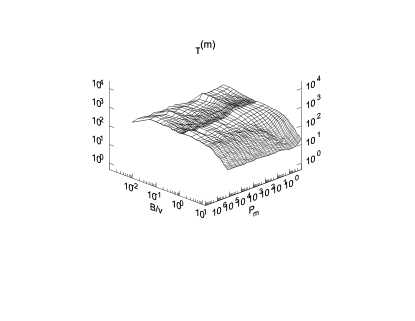
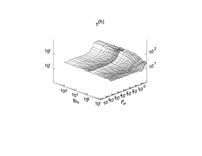
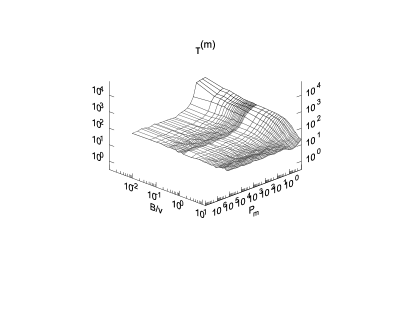
Figure 4: Correlation time. Left - hydrodynamic, right - magnetic. Upper panel: Case 1; lower panel: Case 2

The model (5,1) is clearly a good one when the diffusivities are large, but will not give any better results than the other truncations when the diffusivities are small. Nonetheless it does provide a useful simplification in mid ranges and permits the testing of the various approximations. Plainly a major simplification is that the fields are monochromatic. This could and should be remedied by increasing the number of shells, but this has not yet been attempted.

The model design

Equations (5, 1) were solved numerically using a second order time integration scheme. Time is measured by the typical diffusion time, $t\rightarrow t/\nu$. The random force is normalized with $\nu$ as well, $\mathbf{f}\rightarrow\mathbf{f}\nu$.

The evolution of the small-scale velocity and magnetic fields depends on the typical correlation time of the random force. The time step is $0.003$ (in dimensionless units, time is rescaled according to $t\rightarrow\nu t$). In what follows we consider two different cases. Case 1 is that of zero correlation time: the force is updated at each timestep. In Case 2, which has finite correlation time, the force was updated each 50-th time step.

The effective Reynolds number is given by $Re=u_{c}\ell_{c}/\nu$. In computations presented below we use $\nu=0.05$ and $\nu=0.01$. We define the random driving force by writing $\mathbf{f}^{l}=\mathbf{w}^{(l)}+i\mathbf{k}^{(l)}\times\mathbf{w}^{(l)}$, and similar for initial velocity and magnetic fields. For each $l$ $\mathbf{w}^{(l)}$ is a random vector whose components vary between $\pm 0.5$. The term $i\mathbf{k}^{(l)}\times\mathbf{w}^{(l)}$ is introduced to force positive helicity in the system. The initial velocity field is given helicity of the same sign. The electromotive force associated with the $\left(l\right)-$mode reads

$$\mathcal{E}_{i}^{(l)} = \varepsilon_{ijq}\hat{u}_{j}^{(l)}\widetilde{\hat{b}}_{q}^{(l)}\leavevmode\nobreak\ +c.c.\leavevmode\nobreak\ =\varepsilon_{ijq}\chi_{jq}^{(l)}$$ (11)

where tilde means the complex conjugate. Suppose the mean magnetic field has fixed direction, $\overline{\mathbf{B}}=\mathbf{e}_{x}B_{x}$. The important component of the mean electromotive force is $\mathcal{E}_{x}$, and so we define the $\alpha$ effect via $\alpha={\overline{\mathcal{E}}}_{x}/B_{x}$. The mean electromotive force ${\overline{\mathbf{\mathcal{E}}}}$ is found by summation over all modes and in averaging over the long-time interval equal to about 3000 diffusion times of the system (here $M$ is the total number of time-steps)

$$\overline{\mathcal{E}}_{i}=\varepsilon_{ijq}\frac{1}{M}\sum_{m=0}^{m=M}\sum^{(l)}\chi_{jq}^{(l)}$$ (12)

Typical realizations of $\mathcal{E}_{x}=\varepsilon_{ijq}\sum^{(l)}\chi_{jq}^{n}$ for case $P_{m}=\infty$ and $P_{m}=1$ are shown on the figure 2. The averaging was done over 16 such realizations. For the purpose of comparison we also solve equations (5, 1) using the first order smoothing approximation (FOSA), in which the tensors $\mathcal{M},\mathcal{N}$ are set to zero. To test the $\tau$ approximation we evaluate the third order moments (see explanations above):

$$\chi_{ij}^{(l),\ \tau}=\nu^{-1}\left(\overline{\tilde{M}_{j}^{\left(l\right)}\hat{u}_{i}^{\left(l\right)}}+\overline{\mathcal{N}_{i}^{\left(l\right)}\widetilde{\hat{b}}_{j}^{\left(l\right)}}\right)$$ (13)

Figure 5: $\mathcal{E}$ vs $P_{m}$, $B/\nu=0.1$. Left: Case 1. The FOSA solution is shown by circles, the exact solution by stars and squares show the $\tau$ approximation. The right hand graph shows the same data for Case 2.

Figure 6: $\mathcal{E}_{x}$ vs $B/\nu$. The top row shows comparisons between the full solution of the model and the approximations for Case 1. At left - the case $P_{m}=1$ at right - $P_{m}=10^{3}$. The FOSA solution is shown by circles, the full solution by stars, and squares show the $\tau$ approximation. The bottom shows the same data for Case 2.

First we give a detailed description of results for the case $\nu=0.05$. The results depend very much on whether there is a small-scale dynamo - that is whether a small scale field can exist in the absence of the imposed large scale field. The value of $P_{m}$ affects both the threshold and intensity of the small-scale dynamo. The relation between $P_{m}$ and the amplitude of the small-scale magnetic field fluctuations for $\overline{B}=0$ is shown in Figure 3. For Case 1 there is a small-scale dynamo if $P_{m}\geq 10$. Also, as may be verified directly from the equations, the amplitude of the mean electro-motive force tends to zero if $P_{m}$ approaches infinity. This is illustrated in Figure 5 for the case $B/\nu=1.$ The typical Reynolds number is $Re\approx 2.2$ for Case 1 and $Re\approx 4.8$ for Case 2.

For Case 2 the threshold is about, $P_{m}\approx 1$. We can see that for large $P_{m}$ there is approximate equipartition between the energies of the fluctuating velocity and magnetic field.

As well as examining the accuracy of FOSA, we will explore the usfulness of the $\tau$-approximation. The approximation relies on knowledge of the typical relaxation times $\tau^{(m)},\tau^{(h)}$ of magnetic and hydrodynamic fluctuations. These quantities were found from auto-correlation functions; for $\tau^{(h)}$ we have

$$\mathcal{I}^{\left(h\right)}\left(T\right) = \frac{\overline{\int u_{i}^{\left(l\right)}\left(t\right)u_{i}^{\left(l\right)}\left(t+T\right)dt}}{\overline{\int u_{i}^{\left(l\right)}\left(t\right)u_{i}^{\left(l\right)}\left(t\right)dt}},$$

$$\tau^{\left(h\right)} =T \left(\frac{\mathcal{I}^{\left(h\right)}\left(0\right)}{\mathcal{I}^{\left(h\right)}\left(T\right)}=e^{-1}\right),$$

and similarly for $\tau^{\left(m\right)}$. Both $\tau^{\left(h\right)}$ and $\tau^{\left(m\right)}$ are functions of $\overline{B}$ and $P_{m}$, as shown in Figure 4. As we can see, $\tau^{\left(h\right)}$ depends strongly on $\overline{B}$. Its variation with $P_{m}$ depends on the existence of the small-scale dynamo. On the other hand, $\tau^{\left(m\right)}$ does not show considerable variation either with $\overline{B}$ or $P_{m}$. To estimate the results of $\tau$ approximation we take $\overline{\tau}=\left(\tau^{\left(h\right)}+\tau^{\left(m\right)}\right)/2$.

The dependence of the calculated mean electromotive force on $P_{m}$ for the fixed strength of $\overline{B}$ is shown in Figure5. The maxima are at values of $P_{m}$ that are close to the thresholds for the small-scale dynamo. For high $P_{m}$, $\mathcal{E}$ fluctuates strongly about zero. The dependence of the magnitude of the mean electromotive force on $P_{m}$ is not easily determined for small values of $\overline{B}$ because of strong fluctuations.

To investigate the quenching of the $\alpha$-effect we need to examine the dependence of $\mathcal{E}_{x}$ on $B_{x}$. We approximate this with the following fitting functions, depending on three parameters $A_{1},A_{2},A_{3}$:

$$\frac{A_{1}B}{1+A_{2}B^{A_{3}}}$$ (14)

Examples of these fits for the different cases are shown on the fig6. The fit (14) does not work well for high $P_{m}$ as the mean electromotive force tends to zero and is highly fluctuating. However the limiting behaviour for strong magnetic fields is approximated quite well. The deviation of the FOSA from the exact solution is clearly seen for high conductivity and Case 2. In the same way we can say that the $\tau$ approximation gives a better fit to the exact solution for those parameter values. This is confirmed by the results shown in Figure 7, where we show variations of $A_{1-3}$ with $P_{m}$.

Figure 7: $A_{1,2,3}$ vs $P_{m}$. Top row: Case 1. The FOSA solution is shown by circles, the exact solution by stars, and the $\tau$ approximation by squares. The bottom row shows the same data for Case 2.

Several features are quite well seen in Figure 7. First, in Case 1 the $\tau$ approximation seems bad. Even the sign of effect is opposite to that for the exact solution. On the other hand a significant difference between the exact solution and FOSA is well seen for the high $P_{m}$. Second, “catastrophic quenching”, when $A_{2}\sim R_{m}$, is found for the high-conducting case. This phenomenon is more pronounced for FOSA than for the $\tau$ approximation and the full solution. Third, in Case 1 for FOSA the power $A_{3}$ of quenching function is about $1.8$ in the whole range while for Case 2 it is slightly higher - $2$. The quenching power of the exact and FOSA solutions are close.

Plots of the amplitude of $\mathcal{E}_{x}$ and the alpha-quenching as functions of $P_{m}$ and magnetic field strength $B/\nu$ are shown in Figure 8. Again we see that “catastrophic” quenching occurs for high $P_{m}$.

A formula that is widely quoted and has been justified by use of the $\tau$ approximation is the simple relation between kinetic and current helicities in turbulent flows and the $\alpha$ effect, $\alpha\sim\tau\left(h_{\mathcal{C}}-h_{\mathcal{K}}\right)$, where $h_{\mathcal{C}}=\mu^{-1}\left\langle\mathbf{b\cdot\nabla\times b}\right\rangle$ and $h_{\mathcal{K}}=\left\langle\mathbf{u\cdot\nabla\times u}\right\rangle$Brandenburg and Subramanian (2005); Krause and Rädler (1980); Moffatt (1978); Kuzanyan et al. (2006). In Figure 9 we show the $\alpha$ effect and residual helicity $c\tau^{(h)}\left(h_{\mathcal{C}}-h_{\mathcal{K}}\right)$(with $\tau^{(h)}$ as given in Figure 4) for two cases of the random force driving the turbulence. The coefficient was approximately chosen to match the maximum magnitude of the $\alpha$, we put $c=1/3$ both for Case 1 and for Case 2. Clearly, there is no unique relation between $\alpha$ and residual helicity on the whole range of $P_{m}$. Though there is correspondence in sign.

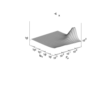
Figure 8: Plots of $-\mathcal{E}_{x}$ (left) and $\alpha$ (right) as functions of $B/v$ and $P_{m}$ for Case 2. Case 1 is similar (sf Figure7).

Figure 9: The alpha effect (dashed line) and residual helicity $c\tau^{(h)}\left(h_{\mathcal{C}}-h_{\mathcal{K}}\right)$ (solid line), for the steady forcing (left) and for the $\delta$-correlated random force (right), as functions of $P_{m}$ and $B/\nu=0.001$.

Next we consider some results for a somewhat higher Reynolds number with $\nu=.01$. Again we present results for two cases. Case 1 is that of zero correlation time: the force is updated at each timestep and $Re\approx 11$. In Case 2, which has finite correlation time, the force was updated each 50-th time step and $Re\approx 22.8$. The relation between $P_{m}$ and the amplitude of the small-scale magnetic field fluctuations for $\overline{B}=0$ is shown in Figure 10. For Case 1 there is a small-scale dynamo if $P_{m}\geq 1$, while it exists for $P_{m}>.1$ in Case 2 . Also in Case 2 we observe that for the high enough $P_{m}$ the energy of magnetic fluctuations is slightly larger than its kinetic counterpart.

Figure 10: $\nu=0.01$, Left: ratio between magnetic and kinetic energy as a function of $P_{m}$. Squares are Case 1 and circles are Case 2. Right: the residual helicity as a function of $P_{m}$: Case 1, dashed line, Case 2, solid line.

This seems to be a main reason why the $\alpha$ effect changes sign as $P_{m}$ varies from low to high values. Meanwhile the residual helicity ($\left(h_{\mathcal{C}}-h_{\mathcal{K}}\right)$) does not. This is demonstrated on Figure11 and helicity is shown at right side on Figure10. The reversal of sign the $\alpha$ effect for high $Rm$ was also found by Courvoisier et al. (2006). Having in mind that the energy of magnetic fluctuations dominates the kinetic energy of the flow we could interpret this on the basis of results of analytical calculations of the $\alpha$ effect for a rotating stratified turbulence within $\tau$- approximation as those given in, e.g., Rädler et al. (2003); Rogachevskii and Kleeorin (2004); Pipin (2007). Suppose that the vector $\mathbf{U}$ characterizes the stratification scale and $\mathbf{\Omega}$ is a global rotation velocity then for the case of slowly rotating media penetrated with a weak large-scale magnetic field, within $\tau$- approximation we obtain $\alpha\sim$$\left(\mathbf{\Omega\cdot U}\right)\tau_{c}^{2}\left({\displaystyle\frac{\left\langle b^{2}\right\rangle}{4\pi\rho}}-\left\langle u^{2}\right\rangle\right)$. However in this theory the sign of expression in the brackets is intimately related to the sign of the residual helicity which is not the case for the computational results presented above. This point needs further clarifications in the multiscale model.

Figure 11: $\nu=0.01$, the mean-electromotive force vs $P_{m}$ with mean field fixed to $B/\nu=0.01$, left is the the Case 1 right - Case 2. We decrease the values of $\mathcal{E}$ obtained from FOSA to factor 10 to make all the curves visible in one scale. Circles show FOSA, stars - exact solution and squares - for the $\tau$-approximation.

Discussion and conclusions

One of the core issues of mean-field dynamo theory is the absence of reliable method for evaluation of the kinetic coefficients which describe the influence of turbulent dynamics on the evolution of the large-scale field. This issue is related to the unsolved closure problem in turbulence theories. Here we have attempted to construct a simple nonlinear dynamical model that can be used for this purpose. The feasibility of the model was demonstrated by numerical calculation of the nonlinear $\alpha$ effect. Moreover, the model is helpful to check two basic analytic ansätze of mean-field magnetohydrodynamics - SOCA(FOSA) and the $\tau$ approximation, at least for moderate values of $R_{m}$. Our results indicate that the $\tau$ approximation may be useful in a dynamical regimes where the small-scale dynamo is active. On the other hand, the results show catastrophic quenching of the $\alpha$ effect for high $P_{m}$. This is not found in analytic computations either in Rogachevskii and Kleeorin (2004) or in Pipin (2007). Certainly the applicability limits of this approximation need further clarification, but we can say with some confidence that if the approximation schemes fail for the present model they are unlikely to be very good for a fully resolved calculation.

In the paper we present numerical calculations of the mean electromotive force for two different temporal regimes of the random force driving the turbulence. One case (Case 1) is essentially white-noise forcing and the other (Case 2) is a coloured noise with a random force which was updated each 50th time step (for our parameters this is about two diffusion times of the system). We found that in the high conductivity limit, the difference between SOCA and the full solution of the model is quite significant. In particular, the full $\alpha$ effect is more than 10 times smaller than that from SOCA. The difference in magnetic quenching is not very large. For high $P_{m}$ the $\alpha$effect is quenched $\alpha\sim\overline{B}^{-4}$ in the nonlinear model though SOCA gives $\alpha\sim\overline{B}^{-3}$ which is consistent with previous findings by Rüdiger and Kichatinov (1993); Sur et al. (2007).

The model is not competent to deal properly with turbulent diffusion because there no energy transfer to different spatial scales. In fact, it would be very useful to generalize the simple Fourier vector space given at Figure 1 to a more general one with several shells. Then the effect of non-uniform magnetic fields and nonuniform flow on the turbulence and the mean electromotive force can be investigated in a similar way. One possible generalisation would be to consider a decomposition of the fluctuating velocity of the form

$$\mathbf{u}\left(\mathbf{x}\right)=\sum_{j=1,3}\sum_{n=1,6}\mathbf{\hat{u}}^{(j,n)}e^{\imath(\mathbf{k}^{(j,n)}\cdot\mathbf{x})}+CC,$$

where for the superscripts $(j,n)$, $j=1,2,3$ is related to the number of a vector shell and $n=1,\ldots 6$ is the number of a mode, and $CC$ denotes complex conjugate. Each shell is similar to that of Figure 1. The modes of these shells interact in each triplet since e.g. $\mathbf{k}^{(1,1)}+\mathbf{k}^{(2,1)}+\mathbf{k}^{(3,1)}=0$ and $\left|\mathbf{k}^{(1,1)}\right|\neq\left|\mathbf{k}^{(2,1)}\right|\neq\left|\mathbf{k}^{(3,1)}\right|$. The dynamical system thus obtained obeys all conservation laws. It should be suitable for the evaluation of $\alpha$ and other effects which are important for the mean-field dynamo, e.g., turbulent diffusion, or joint effect due to global rotation, nonuniform magnetic field and nonuniform mean flow.

Acknowledgements

VVP thanks the Royal Society of London and Trinity College, Cambridge for financial support.

Appendix A

Nonlinear contributions in the induction eq.(5):

$$\mathcal{M}_{i}^{\left(1\right)} = \imath k_{n}^{(1)}\left(\widetilde{\hat{b}}_{n}^{(2)}\hat{u}_{i}^{\left(3\right)}-\widetilde{\hat{b}}_{i}^{(2)}\hat{u}_{n}^{\left(3\right)}+\widetilde{\hat{u}}_{i}^{(2)}\hat{b}_{n}^{\left(3\right)}-\widetilde{\hat{u}}_{n}^{(2)}\hat{b}_{i}^{\left(3\right)}\right.$$

$$\left.+\widetilde{\hat{b}}_{n}^{(4)}\hat{u}_{i}^{\left(5\right)}-\widetilde{\hat{b}}_{i}^{(4)}\hat{u}_{n}^{\left(5\right)}+\widetilde{\hat{u}}_{i}^{(4)}\hat{b}_{n}^{\left(5\right)}-\widetilde{\hat{u}}_{n}^{(4)}\hat{b}_{i}^{\left(5\right)}\right),$$

$$\mathcal{M}_{i}^{\left(2\right)} = \imath k_{n}^{(2)}\left(\widetilde{\hat{b}}_{n}^{(1)}\hat{u}_{i}^{\left(3\right)}-\widetilde{\hat{b}}_{i}^{(1)}\hat{u}_{n}^{\left(3\right)}+\widetilde{\hat{u}}_{i}^{(1)}\hat{b}_{n}^{\left(3\right)}-\widetilde{\hat{u}}_{n}^{(1)}\hat{b}_{i}^{\left(3\right)}\right.$$

$$\left.+\widetilde{\hat{b}}_{n}^{(6)}\hat{u}_{i}^{\left(4\right)}-\widetilde{\hat{b}}_{i}^{(6)}\hat{u}_{n}^{\left(4\right)}+\widetilde{\hat{u}}_{i}^{(6)}\hat{b}_{n}^{\left(4\right)}-\widetilde{\hat{u}}_{n}^{(6)}\hat{b}_{i}^{\left(4\right)}\right),$$

$$\mathcal{M}_{i}^{\left(3\right)} = \imath k_{n}^{(3)}\left(\hat{b}_{n}^{(1)}\hat{u}_{i}^{\left(2\right)}-\hat{b}_{i}^{(1)}\hat{u}_{n}^{\left(2\right)}+\hat{u}_{i}^{(1)}\hat{b}_{n}^{\left(2\right)}-\hat{u}_{n}^{(1)}\hat{b}_{i}^{\left(2\right)}\right.$$

$$\left.+\widetilde{\hat{b}}_{n}^{(6)}\hat{u}_{i}^{\left(5\right)}-\widetilde{\hat{b}}_{i}^{(6)}\hat{u}_{n}^{\left(5\right)}+\widetilde{\hat{u}}_{i}^{(6)}\hat{b}_{n}^{\left(5\right)}-\widetilde{\hat{u}}_{n}^{(6)}\hat{b}_{i}^{\left(5\right)}\right),$$

$$\mathcal{M}_{i}^{\left(4\right)} = \imath k_{n}^{(4)}\left(\hat{b}_{n}^{(6)}\hat{u}_{i}^{\left(2\right)}-\hat{b}_{i}^{(6)}\hat{u}_{n}^{\left(2\right)}+\hat{u}_{i}^{(6)}\hat{b}_{n}^{\left(2\right)}-\hat{u}_{n}^{(6)}\hat{b}_{i}^{\left(2\right)}\right.$$

$$\left.+\widetilde{\hat{b}}_{n}^{(1)}\hat{u}_{i}^{\left(5\right)}-\widetilde{\hat{b}}_{i}^{(1)}\hat{u}_{n}^{\left(5\right)}+\widetilde{\hat{u}}_{i}^{(1)}\hat{b}_{n}^{\left(5\right)}-\widetilde{\hat{u}}_{n}^{(1)}\hat{b}_{i}^{\left(5\right)}\right),$$

$$\mathcal{M}_{i}^{\left(5\right)} = \imath k_{n}^{(5)}\left(\hat{b}_{n}^{(1)}\hat{u}_{i}^{\left(4\right)}-\hat{b}_{i}^{(1)}\hat{u}_{n}^{\left(4\right)}+\hat{u}_{i}^{(1)}\hat{b}_{n}^{\left(4\right)}-\hat{u}_{n}^{(1)}\hat{b}_{i}^{\left(4\right)}\right.$$

$$\left.+\hat{b}_{n}^{(3)}\hat{u}_{i}^{\left(6\right)}-\hat{b}_{i}^{(3)}\hat{u}_{n}^{\left(6\right)}+\hat{u}_{i}^{(3)}\hat{b}_{n}^{\left(6\right)}-\hat{u}_{n}^{(3)}\hat{b}_{i}^{\left(6\right)}\right),$$

$$\mathcal{M}_{i}^{\left(6\right)} = \imath k_{n}^{(6)}\left(\widetilde{\hat{b}}_{n}^{(2)}\hat{u}_{i}^{\left(4\right)}-\widetilde{\hat{b}}_{i}^{(2)}\hat{u}_{n}^{\left(4\right)}+\widetilde{\hat{u}}_{i}^{(2)}\hat{b}_{n}^{\left(4\right)}-\widetilde{\hat{u}}_{n}^{(2)}\hat{b}_{i}^{\left(4\right)}\right.$$

$$\left.+\widetilde{\hat{b}}_{n}^{(3)}\hat{u}_{i}^{\left(5\right)}-\widetilde{\hat{b}}_{i}^{(3)}\hat{u}_{n}^{\left(5\right)}+\widetilde{\hat{u}}_{i}^{(3)}\hat{b}_{n}^{\left(5\right)}-\widetilde{\hat{u}}_{n}^{(3)}\hat{b}_{i}^{\left(5\right)}\right),$$

The nonlinear parts of momentum equation (1):

$$\mathcal{N}_{i}^{\left(1\right)} = \imath k_{n}^{(1)}\left(\widetilde{\hat{b}}_{n}^{(2)}\hat{b}_{i}^{\left(3\right)}+\widetilde{\hat{b}}_{i}^{(2)}\hat{b}_{n}^{\left(3\right)}+\widetilde{\hat{b}}_{n}^{(4)}\hat{b}_{i}^{\left(5\right)}+\widetilde{\hat{b}}_{i}^{(4)}\hat{b}_{n}^{\left(5\right)}\right.$$

$$\left.-\widetilde{\hat{u}}_{n}^{(2)}\hat{u}_{i}^{\left(3\right)}-\widetilde{\hat{u}}_{i}^{(2)}\hat{u}_{n}^{\left(3\right)}-\widetilde{\hat{u}}_{n}^{(4)}\hat{u}_{i}^{\left(5\right)}-\widetilde{\hat{u}}_{i}^{(4)}\hat{u}_{n}^{\left(5\right)}\right),$$

$$\mathcal{N}_{i}^{\left(2\right)} = \imath k_{n}^{(2)}\left(\widetilde{\hat{b}}_{n}^{(1)}\hat{b}_{i}^{\left(3\right)}+\widetilde{\hat{b}}_{i}^{(1)}\hat{b}_{n}^{\left(3\right)}+\widetilde{\hat{b}}_{n}^{(6)}\hat{b}_{i}^{\left(4\right)}+\widetilde{\hat{b}}_{i}^{(6)}\hat{b}_{n}^{\left(4\right)}\right.$$

$$\left.-\widetilde{\hat{u}}_{n}^{(1)}\hat{u}_{i}^{\left(3\right)}-\widetilde{\hat{u}}_{i}^{(1)}\hat{u}_{n}^{\left(3\right)}-\widetilde{\hat{u}}_{n}^{(6)}\hat{u}_{i}^{\left(4\right)}-\widetilde{\hat{u}}_{i}^{(6)}\hat{u}_{n}^{\left(4\right)}\right),$$

$$\mathcal{N}_{i}^{\left(3\right)} = \imath k_{n}^{(3)}\left(\hat{b}_{n}^{(1)}\hat{b}_{i}^{\left(2\right)}+\hat{b}_{i}^{(1)}\hat{b}_{n}^{\left(2\right)}+\widetilde{\hat{b}}_{n}^{(6)}\hat{b}_{i}^{\left(5\right)}+\widetilde{\hat{b}}_{i}^{(6)}\hat{b}_{n}^{\left(5\right)}\right.$$

$$\left.-\hat{u}_{n}^{(1)}\hat{u}_{i}^{\left(2\right)}-\hat{u}_{i}^{(1)}\hat{u}_{n}^{\left(2\right)}-\widetilde{\hat{u}}_{n}^{(6)}\hat{u}_{i}^{\left(5\right)}-\widetilde{\hat{u}}_{i}^{(6)}\hat{u}_{n}^{\left(5\right)}\right),$$

$$\mathcal{N}_{i}^{\left(4\right)} = \imath k_{n}^{(4)}\left(\widetilde{\hat{b}}_{n}^{(1)}\hat{b}_{i}^{\left(5\right)}+\widetilde{\hat{b}}_{i}^{(1)}\hat{b}_{n}^{\left(5\right)}+\hat{b}_{n}^{(6)}\hat{b}_{i}^{\left(2\right)}+\hat{b}_{i}^{(6)}\hat{b}_{n}^{\left(2\right)}\right.$$

$$\left.-\widetilde{\hat{u}}_{n}^{(1)}\hat{u}_{i}^{\left(5\right)}-\widetilde{\hat{u}}_{i}^{(1)}\hat{u}_{n}^{\left(5\right)}-\hat{u}_{n}^{(6)}\hat{u}_{i}^{\left(2\right)}-\hat{u}_{i}^{(6)}\hat{u}_{n}^{\left(2\right)}\right),$$

$$\mathcal{N}_{i}^{\left(5\right)} = \imath k_{n}^{(5)}\left(\hat{b}_{n}^{(1)}\hat{b}_{i}^{\left(4\right)}+\hat{b}_{i}^{(1)}\hat{b}_{n}^{\left(4\right)}+\hat{b}_{n}^{(6)}\hat{b}_{i}^{\left(3\right)}+\hat{b}_{i}^{(6)}\hat{b}_{n}^{\left(3\right)}\right.$$

$$\left.-\hat{u}_{n}^{(1)}\hat{u}_{i}^{\left(4\right)}-\hat{u}_{i}^{(1)}\hat{u}_{n}^{\left(4\right)}-\hat{u}_{n}^{(6)}\hat{u}_{i}^{\left(3\right)}-\hat{u}_{i}^{(6)}\hat{u}_{n}^{\left(3\right)}\right),$$

$$\mathcal{N}_{i}^{\left(6\right)} = \imath k_{n}^{(6)}\left(\widetilde{\hat{b}}_{n}^{(3)}\hat{b}_{i}^{\left(5\right)}+\widetilde{\hat{b}}_{i}^{(3)}\hat{b}_{n}^{\left(5\right)}+\widetilde{\hat{b}}_{n}^{(2)}\hat{b}_{i}^{\left(4\right)}+\widetilde{\hat{b}}_{i}^{(2)}\hat{b}_{n}^{\left(4\right)}\right.$$

$$\left.-\widetilde{\hat{u}}_{n}^{(2)}\hat{u}_{i}^{\left(4\right)}-\widetilde{\hat{u}}_{i}^{(2)}\hat{u}_{n}^{\left(4\right)}-\widetilde{\hat{u}}_{n}^{(3)}\hat{u}_{i}^{\left(5\right)}-\widetilde{\hat{u}}_{i}^{(3)}\hat{u}_{n}^{\left(5\right)}\right),$$

References

• Bohr etย al. [1998] Bohrย T., Jensenย M., Paladinย G., and Vulpianiย A., 1998 Dynamical systems approach to turbulence. Cambridge: Cambridge University Press
• Brandenburg and Subramanian [2005] Brandenburgย A. and Subramanian K., 2005, Phys. Rep., 417, 1
• Courvoisier etย al. [2006] Courvoisierย A., Hughesย D.W., and Tobiasย S.ย M., 2006, Phys.Rev.Lett., 96, 034503
• Gledser etย al. [1981] Gledser E.B., Dolzhanskij F., and Obuhov A.M., 1981, The hydrodynamical type systems and its applications. M.Nauka
• Krause and Rรคdler [1980] Krause F. and Rรคdler K.-H., 1980, Mean-Field Magnetohydrodynamics and Dynamo Theory. Berlin: Akademie-Verlag
• Kuzanyan etย al. [2006] Kuzanyan K.ย M., Pipin V.ย V., and Seehafer N., 2006, Sol.Phys., 233, 185
• Moffatt [1978] Moffatt H.ย K., 1978, Magnetic Field Generation in Electrically Conducting Fluids. Cambridge, England: Cambridge University Press
• Parker [1979] Parker E.ย N., 1979, Cosmical magnetic fields: Their origin and their activity. Oxford: Clarendon Press
• Pipin [2007] Pipin V.ย V., 2008, GAFD, 102 (astroโ€“ph/0606265)
• Proctor [2003] Proctor M.R.E., 2003, Dynamo processes: the interaction of turbulence and magnetic fields. In M.J. Thompson and J.ย Christensen-Dalsgaard, editors, Stellar Astrophysical Fluid Dynamics, pages 143โ€“158. Cambridge University Press
• Rรคdler [1969] Rรคdler K.-H., 1969, Monats. Dt. Akad. Wiss., 11, 194
• Rรคdler etย al. [2003] Rรคdler K.-H., Kleeorin N., and Rogachevskii I., 2003, Geophys. Astrophys. Fluid Dyn., 97, 249
• Rogachevskii and Kleeorin [2003] Rogachevskii I. and Kleeorin N., 2003, Phys. Rev.E, 68, 036301
• Rogachevskii and Kleeorin [2004] Rogachevskii I. and Kleeorin N., 2004, arXiv:astro-ph/0407375v2
• Rรผdiger and Kichatinov [1993] Rรผdiger G. and Kichatinov L.ย L., 1993, Astron. Astrophys., 269, 581
• Sokoloff and Frick [2003] Sokoloff D.D. and Frick P.G., 2003, Astr.Rep., 47, 511
• Sur etย al. [2007] Sur S.,Subramanian K., and Brandenburg A., 2007, Mon. Not. R. Astron. Soc., 376, 3, 1238
• Weiss [1994] Weiss N.O., 1994, Solar and stellar dynamos. In M.R.E Proctor and A.D. Gilbert, editors, Lectures on Solar and Planetary Dynamos, Cambridge University Press, 59