How to measure the effective action for disordered systems

Abstract

In contrast to standard critical phenomena, disordered systems need to be treated via the Functional Renormalization Group. The latter leads to a coarse grained disorder landscape, which after a finite renormalization becomes non-analytic, thus overcoming the predictions of the seemingly exact dimensional reduction. We review recent progress on how the non-analytic effective action can be measured both in simulations and experiments, and confront theory with numerical work.

1 Introduction

When talking to his experimental colleagues about the marvels of field theory and his recent achievements in computing the effective action of his favorite model, the conversation is likely to resemble this:

Theorist: I have a wonderful field theory, I can even calculate the effective action!

Experimentalist: Can I see it in an experiment? Can I measure it?

Theorist: …well, that’s difficult, but it tells you all you want to know …

Experimentalist: okay, I understand, another of these unverifiable predictions, …

Here we will see how to measure it, considering the explicit and far-from-trivial example of elastic manifolds in a disordered environment. Due to a lack of space, we will not be able to give all arguments in the necessary details. We recommend that the reader consults the recent “Basic Recipes and Gourmet Dishes”[1], to which we also refer for a more complete list of references.

2 The disordered systems treated here – our model

   

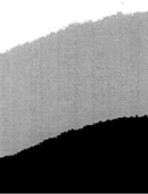
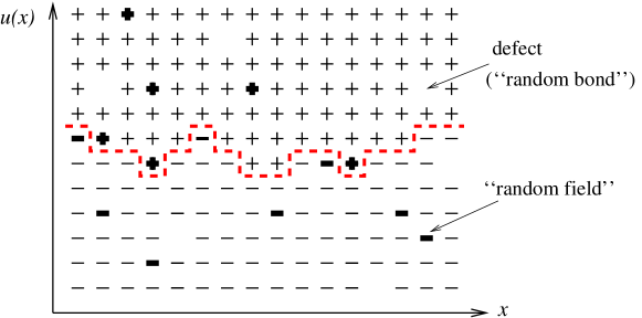
Figure 1: An Ising magnet at low temperatures forms a domain wall described by a function $u(x)$ (right). An experiment on a thin Cobalt film (left) [2]; with kind permission of the authors.

Let us first give some physical realizations. The simplest one is an Ising magnet. Imposing boundary conditions with all spins up at the upper and all spins down at the lower boundary (see figure 1), at low temperature $T$, a domain wall will form in between. In a pure system at $T=0$, this domain wall is completely flat; it will be roughened by disorder. Two types of disorder are common: random bond (which on a course-grained level represents missing spins) and random field (coupling of the spins to an external random magnetic field). Figure 1 shows, how the domain wall is described by a displacement field $u(x)$. Another example is the contact line of water (or liquid hydrogen), wetting a rough substrate. A realization with a 2-parameter field $\vec{u}(\vec{x})$ is the deformation of a vortex lattice: the position of each vortex is deformed from $\vec{x}$ to $\vec{x}+\vec{u}(\vec{x})$. A 3-dimensional example are charge density waves.

All these models are described by a displacement field

$$x\in\mathbb{R}^{d}\ \longrightarrow\ \vec{u}(x)\in\mathbb{R}^{N}\ .$$ (1)

For simplicity, we now set $N=1$. After some initial coarse-graining, the energy ${\cal H}={\cal H}_{\mathrm{el}}+{\cal H}_{\mathrm{DO}}$ consists out of two parts: the elastic energy, and the disorder:

$${\cal H}_{\mathrm{el}}[u]=\int{\mathrm{d}}^{d}x\,\frac{1}{2}\left(\nabla u(x)\right)^{2}\ ,\qquad{\cal H}_{\mathrm{DO}}[u]=\int{\mathrm{d}}^{d}x\,V(x,u(x))\ .$$ (2)

In order to proceed, we need to specify the correlations of disorder[3]:

$$\overline{V(x,u)V(x^{\prime},u^{\prime})}:=\delta^{d}(x-x^{\prime})R(u-u^{\prime})\ .$$ (3)

Fluctuations $u$ in the transversal direction will scale as

$$\overline{\left[u(x)-u(y)\right]^{2}}\sim|x-y|^{2\zeta}\ .$$ (4)

There are several useful observables. We already introduced the roughness-exponent $\zeta$. The second is the renormalized (effective) disorder function $R(u)$, and it is this object we want to measure here. Introducing replicas and averaging over disorder, we can write down the bare action or replica-Hamiltonian

$${\cal H}[u]=\frac{1}{T}\sum_{a=1}^{n}\int{\mathrm{d}}^{d}x\,\frac{1}{2}\left(\nabla u_{a}(x)\right)^{2}-\frac{1}{2T^{2}}\sum_{a,b=1}^{n}\int{\mathrm{d}}^{d}x\,R(u_{a}(x)-u_{b}(x))\ .$$ (5)

Let us stress that one could alternatively pursue a dynamic or a supersymmetric formulation. Since our treatment is perturbative in $R(u)$, the result is unchanged.

3 Dimensional reduction

There is a beautiful and rather mind-boggling theorem relating disordered systems to pure systems (i.e. without disorder), which applies to a large class of systems, e.g. random-field systems and elastic manifolds in disorder. It is called dimensional reduction and reads as follows[4]:

Theorem: A $d$-dimensional disordered system at zero temperature is equivalent to all orders in perturbation theory to a pure system in $d-2$ dimensions at finite temperature.

Experimentally, one finds that this result is wrong, the question being why? Let us stress that there are no missing diagrams or any such thing, but that the problem is more fundamental: As we will see later, the proof makes assumptions, which are not satisfied. Before we try to understand why this is so and how to overcome it, let us give one more example. We know that the width $u$ of a $d$-dimensional manifold at finite temperature in the absence of disorder scales as $u\sim x^{(2-d)/2}$. Making the dimensional shift implied by dimensional reduction leads to

$$\overline{\left[u(x)-u(0)\right]^{2}}\sim x^{4-d}\equiv x^{2\zeta}\quad\mbox{i.e.}\quad\zeta=\frac{4-d}{2}\ .$$ (6)

4 The Larkin-length

To understand the failure of dimensional reduction, let us turn to an interesting argument given by Larkin [5]. He considers a piece of an elastic manifold of size $L$. If the disorder has correlation length $r$, and characteristic potential energy $\bar{f}$, this piece will typically see a potential energy of strength $E_{\mathrm{DO}}=\bar{f}\left(\frac{L}{r}\right)^{\!\frac{d}{2}}.$ On the other hand, there is an elastic energy, which scales like $E_{\mathrm{el}}=c\,L^{d-2}.$ These energies are balanced at the Larkin-length $L=L_{c}$ with $L_{c}=\left(\frac{c^{2}}{\bar{f}^{2}}r^{d}\right)^{\frac{1}{4-d}}.$ More important than this value is the observation that in all physically interesting dimensions $d<4$, and at scales $L>L_{c}$, the membrane is pinned by disorder; whereas on small scales the elastic energy dominates. Since the disorder has a lot of minima which are far apart in configurational space but close in energy (metastability), the manifold can be in either of these minimas, and the ground-state is no longer unique. However exactly this is assumed in the proof of dimensional reduction.

5 The functional renormalization group (FRG)

Let us now discuss a way out of the dilemma: Larkin’s argument suggests that $d=4$ is the upper critical dimension. So we would like to make an $\epsilon=4-d$ expansion. On the other hand, dimensional reduction tells us that the roughness is $\zeta=\frac{4-d}{2}$ (see (6)). Even though this is systematically wrong below four dimensions, it tells us correctly that at the critical dimension $d=4$, where disorder is marginally relevant, the field $u$ is dimensionless. This means that having identified any relevant or marginal perturbation (as the disorder), we can find another such perturbation by adding more powers of the field. We can thus not restrict ourselves to keeping solely the first moments of the disorder, but have to keep the whole disorder-distribution function $R(u)$. Thus we need a functional renormalization group treatment (FRG). Functional renormalization is an old idea, and can e.g. be found in [6]. For disordered systems, it was first proposed in 1986 by D. Fisher [7]. Performing an infinitesimal renormalization, i.e. integrating over a momentum shell à la Wilson, leads to the flow $\partial_{\ell}R(u)$, with ($\epsilon=4-d$)

$$\partial_{\ell}R(u)=\left(\epsilon-4\zeta\right)R(u)+\zeta uR^{\prime}(u)+\frac{1}{2}R^{\prime\prime}(u)^{2}-R^{\prime\prime}(u)R^{\prime\prime}(0)\ .$$ (7)

The first two terms come from the rescaling of $R$ and $u$ respectively. The last two terms are the result of the 1-loop calculations, see e.g. [7, 1].

More important than the form of this equation is it actual solution, sketched in figure 2.

Figure 2: Change of $-R^{\prime\prime}(u)$ under renormalization and formation of the cusp.

After some finite renormalization, the second derivative of the disorder $R^{\prime\prime}(u)$ acquires a cusp at $u=0$; the length at which this happens is the Larkin-length. How does this overcome dimensional reduction? To understand this, it is interesting to study the flow of the second and forth moment. Taking derivatives of (7) w.r.t. $u$ and setting $u$ to 0, we obtain

$$\partial_{\ell}R^{\prime\prime}(0) = \left(\epsilon-2\zeta\right)R^{\prime\prime}(0)+R^{\prime\prime\prime}(0)^{2}\ \longrightarrow\ \left(\epsilon-2\zeta\right)R^{\prime\prime}(0)$$ (8)

$$\partial_{\ell}R^{\prime\prime\prime\prime}(0) = \epsilon R^{\prime\prime\prime\prime}(0)+3R^{\prime\prime\prime\prime}(0)^{2}+4R^{\prime\prime\prime}(0)R^{\prime\prime\prime\prime\prime}(0)\longrightarrow\epsilon R^{\prime\prime\prime\prime}(0)+3R^{\prime\prime\prime\prime}(0)^{2}.$$

Since $R(u)$ is an even function, and moreover the microscopic disorder is smooth (after some initial averaging, if necessary), $R^{\prime\prime\prime}(0)$ and $R^{\prime\prime\prime\prime\prime}(0)$ are 0, which we have already indicated. The above equations for $R^{\prime\prime}(0)$ and $R^{\prime\prime\prime\prime}(0)$ are in fact closed. The first tells us first that the flow of $R^{\prime\prime}(0)$ is trivial and that $\zeta=\epsilon/2\equiv\frac{4-d}{2}$. This is exactly the result predicted by dimensional reduction. The appearance of the cusp can be inferred from the second one. Its solution is $R^{\prime\prime\prime\prime}(0)\hskip 0.43057pt\raisebox{-4.30554pt}[0.0pt][3.44444pt]{\rule{0.43057pt}{11.84024pt}\hskip 0.86108pt}_{\ell}=\frac{c\,{\mathrm{e}}^{\epsilon\ell}}{1-3\,c\left({\mathrm{e}}^{\epsilon\ell}-1\right)/\epsilon}$, with $c=R^{\prime\prime\prime\prime}(0)\hskip 0.43057pt\raisebox{-4.30554pt}[0.0pt][3.44444pt]{\rule{0.43057pt}{11.84024pt}\hskip 0.86108pt}_{\ell=0}$. Thus after a finite renormalization $R^{\prime\prime\prime\prime}(0)$ becomes infinite: The cusp appears. By analyzing the solution of the flow-equation (7), one also finds that beyond the Larkin-length $R^{\prime\prime}(0)$ is no longer given by (8) with $R^{\prime\prime\prime}(0)^{2}=0$. The correct interpretation of (8), which remains valid after the cusp-formation, is $\partial_{\ell}R^{\prime\prime}(0)=\left(\epsilon-2\zeta\right)R^{\prime\prime}(0)+R^{\prime\prime\prime}(0^{+})^{2}.$ Renormalization of the whole function thus overcomes dimensional reduction. The appearance of the cusp also explains why dimensional reduction breaks down: The simplest way to see this is by redoing the proof for elastic manifolds in disorder, which in the absence of disorder is a simple Gaussian theory. Terms contributing to the 2-point function involve $R^{\prime\prime}(0)$, $TR^{\prime\prime\prime\prime}(0)$ and higher derivatives of $R(u)$ at $u=0$, which all come with higher powers of $T$. To obtain the limit of $T\to 0$, one sets $T=0$, and only $R^{\prime\prime}(0)$ remains. This is the dimensional-reduction result. However we just saw that $R^{\prime\prime\prime\prime}(0)$ becomes infinite. Not surprisingly $R^{\prime\prime\prime\prime}(0)T$ may also contributes; indeed one can show that it does, hence the proof fails.

6 The cusp and shocks

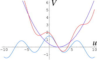
(a) $\quad\stackrel{{\scriptstyle\mbox{\small minimize}}}{{-\!\!\!-\!\!\!-\!\!\!-\!\!\!\longrightarrow}}\quad$ (b)

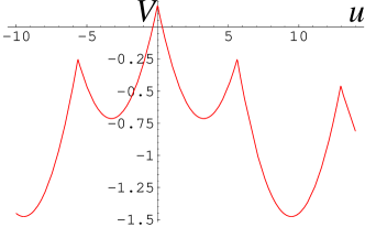
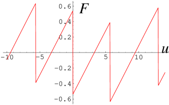
(c) $\quad\stackrel{{\scriptstyle\mbox{\small average}}}{{-\!\!\!-\!\!\!-\!\!\!-\!\!\!\longrightarrow}}\quad$ (d)

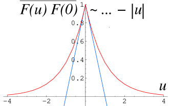
Figure 3: Generation of the cusp, as explained in the main text.

Let us give a simple argument of why a cusp is a physical necessity, and not an artifact. The argument is quite old and appeared probably first in the treatment of correlation-functions by shocks in Burgers turbulence. It was nicely illustrated in [8]. Suppose, we want to integrate out a single degree of freedom coupled with a spring. This harmonic potential and the disorder term are represented by the parabola and the lowest curve on figure 3(a) respectively; their sum is the remaining curve. For a given disorder realization, the minimum of the potential as a function of $u$ is reported on figure 3(b). Note that it has non-analytic points, which mark the transition from one minimum to another. Taking the derivative of the potential leads to the force in figure 3(c). It is characterized by almost linear pieces, and shocks (i.e. jumps). Calculating the force-force correlator, the dominant contribution for small distances is due to shocks. Their contribution is proportional to their probability, i.e. to the distance between the two observable points. This leads to $\overline{F(u)F(0)}=\overline{F(0)^{2}}-c|u|$, with some numerical coefficient $c$.

7 The field-theoretic version

The above toy model can be generalized to the field theory [9]. Consider an interface in a random potential, and add a quadratic potential well, centered around $w$:

$${\cal H}_{\mathrm{tot}}^{w}[u]=\int_{x}\frac{m^{2}}{2}(u(x)-w)^{2}+{\cal H}_{\mathrm{el}}[u]+{\cal H}_{\mathrm{DO}}[u]\ .$$ (9)

In each sample (i.e. disorder configuration), and given $w$, one finds the minimum energy configuration. This ground state energy is

$$\hat{V}(w):=\min_{u(x)}{\cal H}_{\mathrm{tot}}^{w}[u]\ .$$ (10)

It varies with $w$ as well as from sample to sample. Its second cumulant

$$\overline{\hat{V}(w)\hat{V}(w^{\prime})}^{c}=L^{d}R(w-w^{\prime})$$ (11)

defines a function $R(w)$ which is proven [9] to be the same function computed in the field theory, defined from the zero-momentum effective action [10]. Physically, the role of the well is to forbid the interface to wander off to infinity. The limit of small $m$ is taken to reach the universal limit. The factor of volume $L^{d}$ is necessary, since the width $\overline{u^{2}}$ of the interface in the well cannot grow much more than $m^{-\zeta}$. This means that the interface is made of roughly $L/L_{m}$ pieces of internal size $L_{m}\approx m$ pinned independently: (11) expresses the central-limit theorem and $R(w)$ measures the second cumulant of the disorder seen by each piece.

Figure 4: Filled symbols show numerical results for $Y(z)$, a normalized form of the interface displacement correlator $-R^{\prime\prime}(u)$ [Eq. (12)], for $D=2+1$ random field (RF) and $D=3+1$ random bond (RB) disorders. These suggest a linear cusp. The inset plots the numerical derivative $Y^{\prime}(z)$, with intercept $Y^{\prime}(0)\approx-0.807$ from a quadratic fit (dashed line). Open symbols plot the cross-correlator ratio $Y_{s}(z)=\Delta_{12}(z)/\Delta_{11}(0)$ between two related copies of RF disorder. It does not exhibit a cusp. The points are for confining wells with width given by $M^{2}=0.02$. Comparisons to 1-loop FRG predictions (curves) are made with no adjustable parameters. Reprinted from [11].

The nice thing about (11) is that it can be measured. One varies $w$ and computes (numerically) the new ground-state energy; finallying averaging over many realizations. This has been performed recently in [11] using a powerful exact-minimization algorithm, which finds the ground state in a time polynomial in the system size. In fact, what was measured there are the fluctuations of the center of mass of the interface $u(w)=L^{-d}\int{\mathrm{d}}^{d}x\,u_{0}(x;w)$:

$$\overline{[w-u(w)][w^{\prime}-u(w^{\prime})]}^{c}=m^{-4}L^{-d}\Delta(w-w^{\prime})$$ (12)

which measures directly the correlator of the pinning force $\Delta(u)=-R^{\prime\prime}(u)$. To see why it is the total force, write the equilibrium condition for the center of mass $m^{2}[w-u(w)]+L^{-d}\int{\mathrm{d}}^{d}x\,F(x,u)=0$ (the elastic term vanishes if we use periodic b.c.). The result is represented in figure 4. It is most convenient to plot the function $Y=\Delta(u)/\Delta(0)$ and normalize the $u$-axis to eliminate all non-universal scales.

  

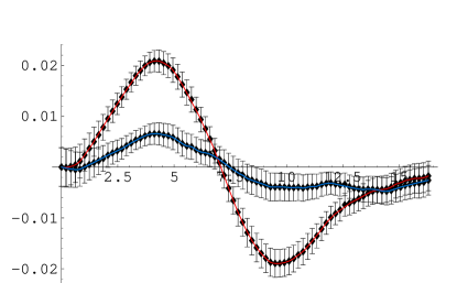
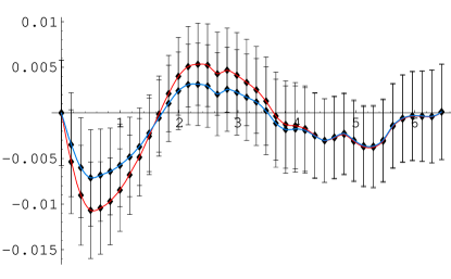
Figure 5: The measured $Y(u)$ with the 1- and 2-loop corrections subtracted. Left: RB-disorder, right: RF-disorder. One sees that the 2-loop corrections improve the precision.

Figure 6: Running the RG in a numerical simulation: Crossover from RB disorder to RF for a driven particle (left)[11]. Residual error for $Y(u)$ for a driven string [12] which show that statics and depinning are controled by different fixed points.

The plot in figure 4 is free of any parameter. It has several remarkable features. First, it clearly shows that a linear cusp exists in any dimension. Next it is very close to the 1-loop prediction. Even more remarkably the statistics is good enough [11] to reliably compare the deviations to the 2-loop predictions of [13].

When we vary the position $w$ of the center of the well, it is not a real motion. It means to find the new ground state for each $w$. Literally “moving” $w$ is another interesting possibility: It measures the universal properties of the so-called “depinning transition” [14, 12]. This was recently implemented numerically (see Fig. 6).

Acknowledgments

It is a pleasure to thank Wolfhard Janke and Axel Pelster, the organizers of PI-2007 for the opportunity to give this lecture. We thank Alan Middleton and Alberto Rosso for fruitful collaborations which allowed to measure the FRG effective action in numerics and Andrei Fedorenko and Werner Krauth for stimulating discussions. This work has been supported by ANR (05-BLAN-0099-01).

References

- [1] K. Wiese and P. L. Doussal, cond-mat/ 0611346 (2006).
- [2] S. Lemerle, J. Ferré, C. Chappert, V. Mathet, T. Giamarchi and P. Le Doussal, Phys. Rev. Lett. 80, p. 849 (1998).
- [3] This is explained in detail in [1].
- [4] K. Efetov and A. Larkin, Sov. Phys. JETP 45, p. 1236 (1977).
- [5] A. Larkin, Sov. Phys. JETP 31, p. 784 (1970).
- [6] F. Wegner and A. Houghton, Phys. Rev. A 8, 401 (1973).
- [7] D. Fisher, Phys. Rev. Lett. 56, 1964 (1986).
- [8] L. Balents, J. Bouchaud and M. Mézard, J. Phys. I (France) 6, 1007 (1996).
- [9] P. Le Doussal, Europhys. Lett. 76, 457 (2006).
- [10] P. L. Doussal, K. Wiese and P. Chauve, Phys. Rev. E , p. 026112 (2004).
- [11] A. Middleton, P. Le Doussal and K. Wiese, Phys. Rev. Lett. 98, p. 155701 (2007).
- [12] A. Rosso, P. Le Doussal and K. Wiese, Phys. Rev. B 75, p. 220201 (2007).
- [13] P. Chauve, P. L. Doussal and K. Wiese, Phys. Rev. Lett. 86, 1785 (2001).
- [14] P. Le Doussal and K. Wiese, EPL 77, p. 66001 (2007).