CALT-68-2666
NI-07085

Integrability of the string worldsheet theory in $AdS_{5}\times S^{5}$ is related to the existence of a flat connection depending on the spectral parameter. The transfer matrix is the open-ended Wilson line of this flat connection. We study the product of transfer matrices in the near-flat space expansion of the $AdS_{5}\times S^{5}$ string theory in the pure spinor formalism. The natural operations on Wilson lines with insertions are described in terms of $r$- and $s$-matrices satisfying a generalized classical Yang-Baxter equation. The formalism is especially transparent for infinite or closed Wilson lines with simple gauge invariant insertions.

1 Introduction

Integrability of superstring theory in $AdS_{5}\times S^{5}$ has been a vital input for recent progress in understanding the AdS/CFT correspondence. However quantum integrability of the string worldsheet sigma-model is far from having been established. The notion of quantum integrability is well developed for relativistic massive quantum field theories, which describe scattering of particles in two space-time dimensions. But the string worldsheet theory is a very special type of a quantum field theory, and certainly not a relativistic massive theory. It may not be the most natural way to think of the string worldsheet theory as describing a system of particles. It may be better to think of it as describing certain operators, or rather equivalence classes of operators. What does integrability mean in this case? Progress in this direction could be key to understanding the exact quantum spectrum, which goes beyond the infinite volume spectrum that is obtained from the asymptotic Bethe ansatz [1, 2].

The transfer matrix usually plays an important role in integrable models, in particular in conformal ones [3]. The renormalization group usually acts nontrivially on the transfer matrix [4, 5]. But the string worldsheet theory is special. The transfer matrix on the string worldsheet is BRST-invariant, and there is a conjecture that it is not renormalized. This was demonstrated in a one-loop calculation in [6].

In this paper we will revisit the problem of calculating the Poisson brackets of the worldsheet transfer matrices [7, 8, 9, 10, 11, 12]. The transfer matrix is a monodromy of a certain flat connection on the worldsheet, which exists because of classical integrability. One can think of it as a kind of Wilson line: given an open contour $C$, we calculate $T[C]=P\exp-\int_{C}J$. Instead of calculating the Poisson bracket we consider the product of two transfer matrices for two different contours, and considering the limit when one contour is on top of another:

At first order of perturbation theory studying this limit is equivalent to calculating the Poisson brackets – we will explain this point in detail. We find that the typical object appearing in this calculation is a dynamical (=field-dependent) R-matrix suggested by J.-M. Maillet [13, 14, 15]. The Maillet approach was discussed recently for the superstring in $AdS_{5}\times S^{5}$ in [16, 10, 12].

The transfer matrix is a parallel-transport type of object. Given two points $x$ and $y$ on the string worldsheet, we can consider the tangent spaces to the target at these two points, $T_{x}(AdS_{5}\times S^{5})$ and $T_{y}(AdS_{5}\times S^{5})$. The transfer matrix allows us to transport various vectors, tensors and spinors between $T_{x}(AdS_{5}\times S^{5})$ and $T_{y}(AdS_{5}\times S^{5})$. This allows to construct operators on the worldsheet by inserting the tangent space objects (for example $\partial_{+}x$) at the endpoints of the Wilson line:

or inside the Wilson line:

We study the products of the simplest objects of this type at the first order of perturbation theory. The results are summarised in Section 2. The subsequent sections contain derivations, the main points are in Sections 4.5 and 6. In Section 8 we discuss the consistency conditions (generalized Yang-Baxter equations).

2 Summary of results

This section contains a summary of our results, and in the subsequent sections we will describe the derivation.

2.1 Definitions

2.1.1 The definition of the transfer matrix

Two dimensional integrable systems are characterized by the existence of certain currents $J^{a}$, which have the property that the transfer matrix

$$T[C]=P\exp\left(-\int_{C}J^{a}e_{a}\right)\,,$$ (2.1)

is independent of the choice of the contour. In this definition $e_{a}$ are generators of some algebra. The algebra usually has many different representations, so the transfer matrix is labelled by a representation. We will write $T_{\rho}[C]$ where the generators $e_{a}$ act in the representation $\rho$.

For the string in $AdS_{5}\times S^{5}$ the algebra is the twisted loop algebra $L\mathfrak{psu(2,2|4)}$ and the coupling of the currents to the generators is the following:

$$J_{+}=(J_{0+}^{[\mu\nu]}-N_{0+}^{[\mu\nu]})e^{0}_{[\mu\nu]}+J_{3+}^{\alpha}e^{-1}_{\alpha}+J_{2+}^{\mu}e^{-2}_{\mu}+J_{1+}^{\dot{\alpha}}e^{-3}_{\dot{\alpha}}+N_{0+}^{[\mu\nu]}e^{-4}_{[\mu\nu]}$$ (2.2)

$$J_{-}=(J_{0-}^{[\mu\nu]}-N_{0-}^{[\mu\nu]})e^{0}_{[\mu\nu]}+J_{1-}^{\alpha}e^{1}_{\dot{\alpha}}+J_{2-}^{\mu}e^{2}_{\mu}+J_{3-}^{\dot{\alpha}}e^{3}_{\alpha}+N_{0-}^{[\mu\nu]}e^{4}_{[\mu\nu]}\,.$$ (2.3)

Here $e^{m}_{a}$ are the generators of the twisted loop algebra. We will use the evaluation representation of the loop algebra. In the evaluation representation $e_{a}^{m}$ are related to the generators of some representation of the finite-dimensional algebra $\mathfrak{psu(2,2|4)}$ in the following way:

$$e^{-3}_{\alpha}=z^{-3}t^{1}_{\alpha},\;\;e^{-2}_{\mu}=z^{-2}t^{2}_{\mu},\;\;e^{1}_{\alpha}=zt^{1}_{\alpha}\;\;\mbox{\it etc.}$$ (2.4)

where $z$ is a complex number, which is called “spectral parameter”. Further details on the conventions can be found in Section 3.1 and in [6].

2.1.2 Setup: expansion around flat space and expansion in powers of fields

The gauge group $\mathfrak{g}_{\bar{0}}\subset\mathfrak{psu(2,2|4)}$ acts on the currents in the following way:

$$\delta_{\xi_{\bar{0}}}J_{\bar{1}}=[\xi_{\bar{0}},J_{\bar{1}}]\;,\;\;\delta_{\xi_{\bar{0}}}J_{\bar{2}}=[\xi_{\bar{0}},J_{\bar{2}}]\;,\;\;\delta_{\xi_{\bar{0}}}J_{\bar{3}}=[\xi_{\bar{0}},J_{\bar{3}}]\;,\;\;$$

$$\delta_{\xi_{\bar{0}}}J_{\bar{0}}=-d\xi_{\bar{0}}+[\xi_{\bar{0}},J_{\bar{0}}]\;,\;\;\;\;\mbox{where }\xi_{\bar{0}}\in\mathfrak{g}_{\bar{0}}\,.$$ (2.5)

In terms of the coordinates of the coset space:

$$J=-dgg^{-1}\;,\;\;g\in PSU(2,2|4)\,.$$ (2.6)

The gauge invariance (2.5) acts on $g$ as follows:

$$g\mapsto hg\;,\;\;h=e^{\xi}\;,\;\;\xi\in\mathfrak{g}_{\bar{0}}\,.$$ (2.7)

There are two versions of the transfer matrix. One is $T$ given by Eq. (2.1) and the other is $g^{-1}Tg$. Notice that $g^{-1}Tg$ is gauge invariant, while $T$ is not. We should think of $T[C]$ as a map from the (supersymmetric) tangent space $T(AdS_{5}\times S^{5})$ at the starting point of $C$ to $T(AdS_{5}\times S^{5})$ at the endpoint of $C$.

The choice of a point in $AdS_{5}\times S^{5}$ leads to the special gauge, which we will use in this paper:

$$g=e^{R^{-1}(\vartheta_{L}+\vartheta_{R})}e^{R^{-1}x}\,.$$ (2.8)

Here $R$ is the radius of AdS space, and it is introduced in (2.8) for convenience. The action has a piece quadratic in $x,\vartheta$ and interactions which we can expand in powers of $x,\vartheta$. There are also pure spinor ghosts $\lambda,w$. All the operators can be expanded in powers of $x,\vartheta,\lambda,w$. We will refer to this expansion as “expansion in powers of elementary fields”, or “expansion in powers of $x$”. Every power of elementary field carries a factor $R^{-1}$. The overall power of $R^{-1}$ is equal to twice the number of propagators plus the number of uncontracted elementary fields. A propagator is a contraction of two elementary fields.

The currents are invariant under the global symmetries, up to gauge transformations. For example the global shift

$$S_{g_{0}}x=x+\xi+{1\over 3R^{2}}[x,[x,\xi]]+\ldots$$ (2.9)

results in the gauge transformation of the currents with the parameter

$$h(\vartheta,x;e^{\xi})=\exp\left(-{1\over 2R^{2}}[x,\xi]+\ldots\right)\,.$$ (2.10)

To have the action invariant we should also transform the pure spinors with the same parameter:

$$\delta_{\xi}\lambda=-\left[{1\over 2R^{2}}[x,\xi]\;,\;\lambda\right],\;\;\;\delta_{\xi}w_{+}=-\left[{1\over 2R^{2}}[x,\xi]\;,\;w_{+}\right]$$ (2.11)

and same rules for $\hat{w}_{-},\hat{\lambda}$.

2.2 Fusion and exchange of transfer matrices

2.2.1 The product of two transfer matrices

Consider the transfer matrix in the tensor product of two representations $\rho_{1}\otimes\rho_{2}$. There are two ways of defining this object. One way is to take the usual definition of the Wilson line

$$P\exp\left(-\int J^{a}(z)e_{a}\right)\,,$$ (2.12)

and use for $e_{a}$ the usual definition of the tensor product of generators of a Lie superalgebra:

$$\rho_{1}(e_{a})\otimes{\bf 1}+(-)^{F\bar{a}}\otimes\rho_{2}(e_{a})\,,$$ (2.13)

where $\bar{a}$ is $0$ if $e_{a}$ is an even element of the superalgebra, and $1$ if $e_{a}$ is an odd element of the superalgebra.

Another possibility is to consider two Wilson lines $T_{\rho_{1}}$ and $T_{\rho_{2}}$ and put them on top of each other. In other words, consider the product $T_{\rho_{2}}T_{\rho_{1}}$. In the classical theory these two definitions of the “composite” Wilson line are equivalent, because of this identity:

$$e^{\alpha}\otimes e^{\beta}=e^{\alpha\otimes 1+1\otimes\beta}\,.$$ (2.14)

But at the first order in $\hbar$ there is a difference. The difference is related to the singularities in the operator product of two currents.

Consider the example when the product of the currents has the following form:

$$J^{a}_{+}(w)J^{b}_{+}(0)={1\over w}A^{ab}_{c}J^{c}_{+}+\ldots\,,$$ (2.15)

where dots denote regular terms. Take two contours $C_{1}$ and $C_{2}$ and calculate the product

$$T_{\rho_{2}}[C_{2}]\;T_{\rho_{1}}[C_{1}]\,,$$ (2.16)

where the indices $\rho_{1}$ and $\rho_{2}$ indicate that we are calculating the monodromies in the representations $\rho_{1}$ and $\rho_{2}$ respectively. For example, suppose that the contour $C_{1}$ is the line $\tau=0$ (and $\sigma$ runs from $-\infty$ to $+\infty$), and the contour $C_{2}$ is at $\tau=y$ (and $\sigma\in[-\infty,+\infty]$). Suppose that we bring the contour of $\rho_{2}$ on top of the contour of $\rho_{1}$, in other words $y\to 0$. Let us expand both $T_{\rho_{2}}[C_{2}]$ and $T_{\rho_{1}}[C_{1}]$ in powers of $R^{-2}$, and think of them as series of multiple integrals of $J$. Consider for example a term in which one $\int J$ comes from $T_{\rho_{2}}[C_{2}]$ and another $\int J$ comes from $T_{\rho_{1}}[C_{1}]$. We get:

$$\int\int d\sigma_{1}d\sigma_{2}\;J_{+}^{a}(y,\sigma_{2})(e_{a}\otimes 1)\;J_{+}^{b}(0,\sigma_{1})(1\otimes e_{b})=$$

$$\int\int d\sigma_{1}d\sigma_{2}\;{1\over\sigma_{2}-\sigma_{1}+iy}A^{ab}_{c}J^{c}_{+}\;(e_{a}\otimes 1)(1\otimes e_{b})\,.$$ (2.17)

The pole ${1\over\sigma_{2}-\sigma_{1}+iy}$ leads to the difference between $\lim_{y\to 0}T_{\rho_{2}}[C+y]T_{\rho_{1}}[C]$ and $T_{\rho_{2}\otimes\rho_{1}}[C]$. Indeed, the natural definition of the double integral when $y=0$ would be that when $\sigma_{1}$ collides with $\sigma_{2}$ we take a principle value:

$$\mbox{V.P.}\int\int d\sigma_{1}d\sigma_{2}\;J_{+}^{a}(0,\sigma_{2})(e_{a}\otimes 1)\;J_{+}^{b}(0,\sigma_{1})(1\otimes e_{b})\,.$$ (2.18)

Here V.P. means that we treat the integral as the principal value when $\sigma_{1}$ collides with $\sigma_{2}$. Modulo the linear divergences, which we neglect, the integral (2.18) is finite. This is because $e_{a}\otimes 1$ commutes with $1\otimes e_{b}$. But such a VP integral is different from what we would get in the limit $y\to 0$, by a finite piece. Indeed:

$$\int dwJ_{+}^{a}(w+i\epsilon)J_{+}^{b}(0) = \mbox{V.P.}\int dwJ_{+}^{a}(w)J_{+}^{b}(0)+$$ (2.20)

$$+\pi iA^{ab}_{c}J_{+}^{c}(0)\,.$$

The second row is the difference between the VP prescription and the $\lim\limits_{y\to 0}$ prescription. The additional piece $\pi iA^{ab}_{c}J_{+}^{c}(0)$ could also be interpreted as the deformation of the generator to which $J_{+}^{c}$ couples in the definition of the transfer matrix:

$$J_{+}^{c}(e_{c}\otimes 1+(-)^{F\bar{c}}\otimes e_{c})\mapsto J_{+}^{c}\left(e_{c}\otimes 1+(-)^{F\bar{c}}\otimes e_{c}+\pi iA^{ab}_{c}e_{a}(-)^{F\bar{b}}\otimes e_{b}\right)\,.$$ (2.21)

We have two different definitions of the transfer matrix in the tensor product of two representations. Is it true that these two definitions actually give the same object? There are several logical possibilities:

1. There are several ways to define the transfer matrix, and they all give essentially different Wilson line-like operators.

2. We should interpret Eq. (2.21) as defining the deformed coproduct on the algebra of generators. The algebra of generators is in our case a twisted loop algebra of $\mathfrak{psu(2,2|4)}$. There are at least three possibilities:

   1. The proper definition of the transfer matrix actually requires the deformation of the algebra of generators $e^{a}$, and the deformed algebra has deformed coproduct.

   2. The algebra of generators is the usual loop algebra, but it has a nonstandard coproduct; $\lim_{y\to 0}T_{\rho_{2}}[C+y]T_{\rho_{1}}[C]$ is different from $T_{\rho_{1}\otimes\rho_{2}}[C]$, the difference being the use of a nonstandard coproduct. We are not aware of a mathematical theorem which forbids such a nontrivial coproduct.

   3. The coproduct defined by Eq. (2.21) is equivalent to the standard one, in a sense that it is obtained from the standard coproduct by a conjugation:

      $$\Delta^{0}(e^{c}) = e_{c}\otimes 1+(-)^{F\bar{c}}\otimes e_{c}$$ (2.22)

      $$\Delta(e^{c}) = e_{c}\otimes 1+(-)^{F\bar{c}}\otimes e_{c}+\pi iA^{ab}_{c}e_{a}\otimes(-)^{F\bar{c}}e_{b}=$$ (2.23)

      $$= e^{{\pi i\over 2}r}(e_{c}\otimes 1+(-)^{F\bar{c}}\otimes e_{c})e^{-{\pi i\over 2}r}\,.$$

We will argue that what actually happens (at the tree level) is a generalization of 2c. The deformation (2.23) is almost enough to account for the difference between $\lim_{y\to 0}T_{\rho_{2}}[C+y]T_{\rho_{1}}[C]$ and $T_{\rho_{1}\otimes\rho_{2}}[C]$, but in addition to (2.23) one has to do a field-dependent generalized gauge transformation. The correct statement is:

for a contour $C$ going from the point $A$ to the point $B$

$$\lim_{y\to 0}T_{\rho_{2}}[C+y]T_{\rho_{1}}[C]=e^{{\pi i\over 2}\hat{r}(A)}T_{\rho_{1}\otimes\rho_{2}}[C]e^{-{\pi i\over 2}\hat{r}(B)}$$ (2.24)

where $\hat{r}$ is field dependent (“dynamical”). In fact $\hat{r}$ is of the order $\hbar$. This paper is all about the tree level. Therefore all we are saying is:

$$\lim_{y\to 0}T_{\rho_{2}}[C+y]T_{\rho_{1}}[C]=T_{\rho_{1}\otimes\rho_{2}}[C]+{\pi i\over 2}\left(\;\hat{r}(A)\;T_{\rho_{1}\otimes\rho_{2}}[C]-T_{\rho_{1}\otimes\rho_{2}}[C]\;\hat{r}(B)\;\right)+\ldots$$ (2.25)

where dots stand for loop effects. The hat over the letter $r$ shows that this is a field-dependent object. We will also use a field-independent $r$-matrix which will be denoted $r$ without a hat; $r$ is the leading term in the near-flat-space expansion of $\hat{r}$, which is the expansion in powers of elementary fields explained in Section 2.1.2:

$$\hat{r}\;\;\;= r -{\pi i\over 2}\left(\;((z_{1}^{-2}-z_{1}^{2})t^{2})\otimes[t^{2},x]-[t^{2},x]\otimes((z_{2}^{-2}-z_{2}^{2})t^{2})\;\right)-$$ (2.26)

$$-{\pi i\over 2}\left(\;((z_{1}^{-3}-z_{1})t^{1})\otimes\{t^{3},\vartheta_{L}\}-\{t^{3},\vartheta_{L}\}\otimes((z_{2}^{-3}-z_{2})t^{1})\;\right)-$$

$$-{\pi i\over 2}\left(\;((z_{1}^{-1}-z_{1}^{3})t^{3})\otimes\{t^{1},\vartheta_{R}\}-\{t^{1},\vartheta_{R}\}\otimes((z_{2}^{-1}-z_{2}^{3})t^{3})\;\right)+$$

$$+\ldots$$

Here $r$ is given by Eq. (2.33) and dots stand for the terms of quadratic and higher orders in $x$ and $\vartheta$. The pure spinor ghosts do not enter into the expression for $\hat{r}$, only the matter fields $x$ and $\vartheta$.

Figure 1: Fusion of transfer matrices.

Figure 2: Exchange of transfer matrices.

The special thing about the constant term $r$ is that it is a rational function of the spectral parameter with the first order pole at $z_{u}=z_{d}$. The coefficients of the $x,\vartheta$-dependent terms are all polynomials in $z_{u},z_{d},z_{u}^{-1},z_{d}^{-1}$. The field dependence of the $\hat{r}$ matrix in this example is related to the fact that the pair of Wilson lines with “loose ends” is not a gauge invariant object.

Eq. (2.24) is schematically illustrated in Figure 2. A consequence of (2.24) is the equivalence relation for the exchange of the order of two transfer matrices, see Figure 2:

$$\lim_{C_{u}\searrow C_{d}}T_{C_{u}}({\rho_{u}^{z_{u}}})T_{C_{d}}({\rho_{d}^{z_{d}}})=\exp(\pi i\;\hat{r})\left[\lim_{C_{u}\nearrow C_{d}}T_{C_{u}}({\rho_{u}^{z_{u}}})T_{C_{d}}({\rho_{d}^{z_{d}}})\right]\exp(-\pi i\;\hat{r})\,.$$ (2.27)

2.2.2 Relation to Poisson brackets

At the tree level the calculation of the fusion of transfer matrices is equivalent to the calculation of the Poisson brackets. This follows from the definition of the Poisson bracket:

$$\{T_{\rho_{1}},T_{\rho_{2}}\}=\lim_{\hbar\to 0}{1\over i\hbar}\left(\lim_{y\to 0+}T_{\rho_{1}}[C+y]T_{\rho_{2}}[C]-\lim_{y\to 0+}T_{\rho_{2}}[C+y]T_{\rho_{1}}[C]\right)$$ (2.28)

and the equation:

$$\lim_{y\to 0+}T_{\rho_{1}}[C+y]T_{\rho_{2}}[C]+\lim_{y\to 0+}T_{\rho_{2}}[C+y]T_{\rho_{1}}[C]=2T_{\rho_{1}\otimes\rho_{2}}[C]+O(\hbar^{2})$$ (2.29)

which holds to the first order in $\hbar$. These two equations and Eq. (2.25) imply

$$\{T_{\rho_{1}}[C],T_{\rho_{2}}[C]\}=\pi\left(\;\hat{r}(A)\;T_{\rho_{1}\otimes\rho_{2}}[C]-T_{\rho_{1}\otimes\rho_{2}}[C]\;\hat{r}(B)\;\right)$$ (2.30)

and therefore the calculation of $\hat{r}$ is actually equivalent to the calculation of the Poisson brackets.

To derive (2.29) we expand the product $T[C+y]T[C]$ as normal ordered product plus contractions. At the tree level only one contraction is needed; schematically we get

$$J(w)J(0)=:J(w)J(0):+F(w,\bar{w})$$

where $F(w,\bar{w})$ is $1\over w$ or $1\over w^{2}$ or $1\over\bar{w}$ or $1\over\bar{w}^{2}$ times some expression regular at $w\to 0$; see Section 3. Then eq. (2.29) follows from the relation

$$\hbox{lim}_{\epsilon\rightarrow 0^{+}}\left({1\over(w+i\epsilon)^{n}}+{1\over(w-i\epsilon)^{n}}\right)=2\mbox{V.P.}{1\over w^{n}}$$ (2.31)

applied to the singular part of $F(w,\bar{w})$.

The ”standard” calculation of the Poisson bracket of two transfer matrices involves the equal time Poisson brackets of the currents $\{J(\sigma),J(\sigma^{\prime})\}$. This is proportional to $\delta(\sigma-\sigma^{\prime})$ or $\partial_{\sigma}\delta(\sigma-\sigma^{\prime})$. This is equivalent to what we are doing because:

$$\hbox{lim}_{\epsilon\rightarrow 0^{+}}\left({1\over(w+i\epsilon)^{n}}-{1\over(w-i\epsilon)^{n}}\right)={2\pi i(-1)^{n}\over(n-1)!}\;\partial_{\sigma}\delta(\sigma-\sigma^{\prime})$$ (2.32)

We conclude that the difference between our approach based on the notion of ”fusion” and the ”standard” approach to calculating the Poisson brackets is a matter of notations. (But we believe that our notations are more appropriate for calculating beyond the tree level.)

2.2.3 $r$- and $s$-matrices and generalized classical YBE

The open ended contours like the ones shown in Figures 2 and 2 are strictly speaking not gauge invariant. In our approach we fix the gauge (2.8) and therefore it is meaningful to consider these operators as operators in the gauge fixed theory. Nevertheless we feel that these are probably not the most natural objects to study, at least from the point of view of the differential geometry of the worldsheet.

Figure 3: An infinite Wilson line with an operator insertion

The natural objects to consider are infinite (or periodic) Wilson lines with various operator insertions, see Figure 3. How to describe the algebra formed by such operators? What is the relation between and   ?    We will find that the description of this algebra involves matrices $r$ and $s$ which have the following form:

$$r = {\Phi(z_{1},z_{2})\over z_{1}^{4}-z_{2}^{4}}(z_{1}z_{2}^{3}t^{1}\otimes t^{3}+z_{1}^{3}z_{2}t^{3}\otimes t^{1}+z_{1}^{2}z_{2}^{2}t^{2}\otimes t^{2})+2{\Psi(z_{1},z_{2})\over z_{1}^{4}-z_{2}^{4}}t^{0}\otimes t^{0}\,,$$ (2.33)

$$s = (z_{1}^{-1}z_{2}^{-3}-z_{1}^{3}z_{2})t^{3}\otimes t^{1}+(z_{1}^{-2}z_{2}^{-2}-z_{1}^{2}z_{2}^{2})t^{2}\otimes t^{2}+(z_{1}^{-3}z_{2}^{-1}-z_{1}z_{2}^{3})t^{1}\otimes t^{3}\,,$$ (2.34)

where

$$\Phi(z_{1},z_{2}) = (z_{1}^{2}-z_{1}^{-2})^{2}+(z_{2}^{2}-z_{2}^{-2})^{2}$$

$$\Psi(z_{1},z_{2}) = 1+z_{1}^{4}z_{2}^{4}-z_{1}^{4}-z_{2}^{4}\,.$$

The notations used in (2.33), (2.34) are explained in Section 3.1. In section 8 we will study the consistency conditions for $r$ and $s$, which generalize the standard classical Yang-Baxter algebra. At the tree level we will get a generalization of the classical Yang-Baxter equations:

$$[(r_{12}+s_{12}),(r_{13}+s_{13})]+[(r_{12}+s_{12}),(r_{23}+s_{23})]+[(r_{13}+s_{13}),(r_{23}-s_{23})]=t_{123}\,,$$ (2.35)

where the RHS is essentially a gauge transformation; the explicit expression for $t$ is (8.1). Note that neither $r$ nor $s$ satisfy the standard classical YBE on their own, and even the combination $r\pm s$ satisfies an analogue of the cYBE only when acting on gauge invariant quantities. Therefore we have a generalization of the classical Yang-Baxter equations with the gauge invariance built in.

2.3 Infinite Wilson lines with insertions

To explain how $r$ and $s$ enter in the description of the algebra of transfer matrices, we have to introduce some notations.

2.3.1 General definitions

Consider a Wilson line with an operator insertion, shown in Fig. 3. For this object to be gauge invariant, we want ${\cal O}$ to transform under the gauge transformations in the representation $\rho^{\prime}\otimes\rho^{*}$ of the gauge group $\mathfrak{g}_{\bar{0}}\subset\mathfrak{psu(2,2|4)}$. We will introduce the notation ${\bf H}(\rho_{1}\otimes\rho_{2})$ for the space of operators transforming in the representation $\rho_{1}\otimes\rho_{2}$ of $\mathfrak{g}_{0}$. With this notation:

$${\cal O}\in{\bf H}(\rho^{\prime}\otimes\rho^{*})\,.$$ (2.36)

Here $\rho^{*}$ means the representation dual to $\rho$.

For example, we can take $\rho$ the evaluation representation of the loop algebra corresponding to the adjoint of $\mathfrak{psu(2,2|4)}$, with some spectral parameter $z$, and take ${\cal O}=J_{2+}$:

$$J_{2+}\in{\bf H}(\mbox{ad}^{z}\otimes(\mbox{ad}^{z})^{*})\,.$$ (2.37)

In other words, consider:

$$P\exp\left(-\int_{0}^{+\infty}\mbox{ad}(J(z))\right)\;\mbox{ad}(J_{\bar{2}+})\;P\exp\left(-\int_{-\infty}^{0}\mbox{ad}(J(z))\right)\,.$$ (2.38)

This is gauge invariant because $\mbox{ad}\subset\mbox{ad}\otimes\mbox{ad}^{*}$ as a representation of $\mathfrak{psu}(2,2|4)$ and therefore also as a representation of $\mathfrak{g}_{\bar{0}}$. Of course, we could also pick ${\cal O}=\mbox{ad}(J_{\bar{1}+})$ or $\mbox{ad}(J_{\bar{3}+})$. These operators have engineering dimension $(1,0)$. Geometrically they correspond to $\partial_{+}x$ or $\partial_{+}\vartheta$.

Figure 4: Fusion operations $\mathcal{F}_{+}$, $\mathcal{F}_{-}$ and $\mathcal{G}_{+}$

We want to study the objects of this type in the situation when two contours come close to each other. For example, consider a Wilson line in the representation $\rho_{u}$ with some operator ${\cal O}$ inserted at the endpoint. Let us take another Wilson line, an infinite one, carrying the representation $\rho_{d}$, and put the Wilson line with the representation $\rho_{u}$ on top of the the one carrying $\rho_{d}$. In the limit when the separation goes to zero we should have a Wilson line carrying $\rho_{u}\otimes\rho_{d}$ at $-\infty$ and $\rho_{d}$ at $+\infty$.

This defines maps ${\cal F}_{\pm}$, see Figure 4. If ${\cal O}$ is inserted inside the contour (rather than at the endpoint) we get ${\cal G}_{\pm}$. To summarize:

$${\cal F}_{+}\; : \;{\bf H}(\rho_{u}^{*})\to{\bf H}(\rho_{u}^{*}\otimes\rho_{d}^{*}\otimes\rho_{d})$$ (2.39)

$${\cal F}_{-}\; : \;{\bf H}(\rho_{d}^{*})\to{\bf H}(\rho_{u}^{*}\otimes\rho_{d}^{*}\otimes\rho_{u})$$ (2.40)

$${\cal G}_{+}\; : \;{\bf H}(\rho_{u}^{*}\otimes\rho_{u}^{\prime})\to{\bf H}(\rho_{u}^{*}\otimes\rho_{d}^{*}\otimes\rho_{u}^{\prime}\otimes\rho_{d})$$ (2.41)

$${\cal G}_{-}\; : \;{\bf H}(\rho_{d}^{*}\otimes\rho_{d}^{\prime})\to{\bf H}(\rho_{u}^{*}\otimes\rho_{d}^{*}\otimes\rho_{u}\otimes\rho_{d}^{\prime})\,.$$ (2.42)

2.3.2 Split operators

We also want to be able to insert two operators: ${\cal O}^{i}_{up}$ into the upper line, and ${\cal O}^{j}_{dn}$ into the lower line, such that they are not separately gauge invariant, but $\sum_{i}{\cal O}^{i}_{up}{\cal O}^{i}_{dn}$ is gauge invariant. For example, for a gauge invariant operator ${\cal O}$ we can insert ${\cal C}^{\mu\nu}t^{2}_{\mu}\otimes\{t^{2}_{\nu},{\cal O}\}$ where ${\cal C}_{\mu\nu}={\cal C}_{\mu\nu}(x_{up},x_{dn},\vartheta_{up},\vartheta_{dn})$ is some kind of a parallel transport. This will be gauge invariant. We will use a thin vertical line to denote such a “split operator”

In the tensor product notations, for example when we write ${\cal C}^{\mu\nu}t^{2}_{\mu}\otimes\{t^{2}_{\nu},{\cal O}\}$, we assume that the first tensor generator in the tensor product (in this case $t^{2}_{\mu}$) acts on the upper Wilson line, and the second (in this case $\{t^{2}_{\nu},{\cal O}\}$) on the lower line. We will need such operators in the limit where the upper contour approaches the lower contour. Strictly speaking the split operator will depend on which parallel transport is used even in the limit of coinciding contours, by the mechanism similar to what we described in Section 2.2.1. We will not discuss this dependence in this paper, because it is not important at the tree level.

The exchange map ${\cal R}$ acts as follows:

$${\cal R}\;:\;{\bf H}_{split}(\rho_{1}^{out}\otimes(\rho_{1}^{in})^{*},\rho_{2}^{out}\otimes(\rho_{2}^{in})^{*})\to{\bf H}_{split}(\rho_{2}^{out}\otimes(\rho_{2}^{in})^{*},\rho_{1}^{out}\otimes(\rho_{1}^{in})^{*})\,.$$ (2.43)

The pictorial representation of $\cal R$ is:

2.3.3 Switch operators

Given $\rho$ a representation of $\mathfrak{psu(2,2|4)}$ we denote the evaluation representation $\rho^{z}$. Consider $\rho_{u}=\rho^{z_{u}^{in}}$, $\rho^{\prime}_{u}=\rho^{z_{u}^{out}}$ and $\rho_{d}=\rho^{z_{d}}$, where $z_{u}^{in}$, $z_{u}^{out}$ and $z_{d}$ are three different complex numbers. Take ${\cal O}=1$. This is gauge invariant because $\rho^{z_{u}^{in}}$ and $\rho^{z_{u}^{out}}$ are equivalent as representations of the gauge group $\mathfrak{g}_{0}$. We can think of such ${\cal O}$ as “the operator changing the spectral parameter”, or the “switch operator”

For abbreviation we write $\rho^{in}_{u}=\rho^{z_{u}^{in}}$ and $\rho^{out}_{u}=\rho^{z_{u}^{out}}$. Let us first consider the operation $\mathcal{G}_{+}$ in Figure 4, with $\mathcal{O}=1$. In Section 6.1 we will show that ${\cal G}_{+}({\bf 1})$ is given (at the tree level) by this formula:

$${\cal G}_{+}(1) = {\bf 1}+{\pi i\over 2}\left[(r+s)|_{\rho_{u}^{in}\otimes{\rho_{d}}}-(r+s)|_{\rho_{u}^{out}\otimes{\rho_{d}}}\right]+\ldots$$ (2.44)

Here the $r$ matrix appears from the diagrams involving the interaction of currents in the bulk of the contours. It comes from the deformed coproduct, see Eq. (2.23). The matrix $s$ comes from the diagrams which are localized near the insertion of ${\cal O}$. These are the additional diagrams existing because we inserted the impurities.

The corresponding exchange relation is:

where

$${\cal R}({\bf 1}_{switch}\otimes{\bf 1}) = 1+\pi i\;r_{+}(z_{up}^{in},z_{dn})-\pi i\;r_{+}(z_{up}^{out},z_{dn})+\ldots$$ (2.45)

$$r_{+} = r+s\,.$$

Similarly, if we lift the switched contour from the lower position to the upper position, we should insert ${\cal R}({\bf 1}\otimes{\bf 1}_{switch})$:

$${\cal R}({\bf 1}\otimes{\bf 1}_{switch}) = 1+\pi i\;r_{-}(z_{up}^{in},z_{dn})-\pi i\;r_{-}(z_{up}^{out},z_{dn})+\ldots$$ (2.46)

$$r_{-} = r-s\,.$$

It is useful to write down explicit formulas for $r_{\pm}=r\pm s$ following from (2.33) and (2.34):

$$\left.{r+s\over 2}\right|_{\rho_{u}\otimes\rho_{d}} = {1\over z_{u}^{4}-z_{d}^{4}}\left[(z_{d}^{2}-z_{d}^{-2})^{2}(z_{u}z_{d}^{3}t^{1}\otimes t^{3}+z_{u}^{2}z_{d}^{2}t^{2}\otimes t^{2}+z_{u}^{3}z_{d}t^{3}\otimes t^{1})+\right.$$ (2.47)

$$\phantom{2\over z_{u}^{4}-z_{d}^{4}}\left.+z_{u}^{2}z_{d}^{2}(z_{u}^{2}-z_{u}^{-2})(z_{d}^{2}-z_{d}^{-2})t^{0}\otimes t^{0}\right]\,,$$

$$\left.{r-s\over 2}\right|_{\rho_{u}\otimes\rho_{d}} = {1\over z_{u}^{4}-z_{d}^{4}}\left[(z_{u}^{2}-z_{u}^{-2})^{2}(z_{u}z_{d}^{3}t^{1}\otimes t^{3}+z_{u}^{2}z_{d}^{2}t^{2}\otimes t^{2}+z_{u}^{3}z_{d}t^{3}\otimes t^{1})+\right.$$ (2.48)

$$\phantom{2\over z_{u}^{4}-z_{d}^{4}}\left.+z_{u}^{2}z_{d}^{2}(z_{u}^{2}-z_{u}^{-2})(z_{d}^{2}-z_{d}^{-2})t^{0}\otimes t^{0}\right]\,.$$

We will use the notation

$$R_{+} = {\cal R}({\bf 1}_{switch}\otimes{\bf 1})$$ (2.49)

$$R_{-} = {\cal R}({\bf 1}\otimes{\bf 1}_{switch})\,.$$ (2.50)

2.3.4 Intersecting Wilson lines

In this paper we mostly consider exchange and fusion as relations in the algebra generated by transfer matrices with insertions. It is also possible to think of these operations as defining vertices connecting several Wilson lines in different representations. For example the fusion can be thought of as a triple vertex:

Such vertices will become important if we want to consider networks of Wilson lines. We want to define this triple vertex so that the diagram is indepependent of the position of the vertex, just as it is independent of the shape of the contours. At the tree level we suggest the following prescription:

The subscripts “go-around” and “V.P.” require explanation. They indicate different prescriptions for dealing with the collisions of the currents coupled to $t\otimes 1$ with the currents coupled to $1\otimes t$. Suppose that we consider the integral $\int dw\;J_{a}\;t^{a}\otimes 1$ and the integration contour has to pass through several insertions of $J_{b}\;1\otimes t^{b}$. The prescription is such that to the right of the point $V$ we treat the collision as the principal value integral, while to the left of $V$ the contour for $\int dw(J^{a}t_{a})\otimes 1$ it goes around the singularity in the upper half-plane:

The insertion of $1+{\hat{r}\over 2}$ is necessary to have independence of the position of the vertex $V$. Notice that in defining the worldsheet fusion we use $r$ rather than $r+s$ or $r-s$. This is different from the formula (2.44) for ${\cal G}_{+}$ which uses $r+s$.

2.4 Outline of the calculation

2.4.1 Use of flat space limit

We will use the near flat space expansion of $T[C+y]T[C]$, see Section 2.1.2. For our calculation it is important that the transfer matrix is undeformable. The definition given by Eqs. (2.1), (2.2) and (2.3) cannot be modified in any essential way. More precisely, we will use the following statement. Suppose that there is another definition of the contour independent Wilson line of the form

$$T^{new}=P\exp\left(-\int_{C}I^{a}e_{a}\right)\,,$$ (2.51)

where the new currents $I$ have ghost number zero and coincide with $J$ at the lowest order in the near flat space expansion. In other words:

$$I_{0\pm}=0+\ldots\;,\;\;I_{1\pm}=-{1\over R}\partial_{\pm}\vartheta_{R}+\ldots\;,\;\;I_{2\pm}=-{1\over R}\partial_{\pm}x+\ldots\;,\;\;I_{3\pm}=-{1\over R}\partial_{\pm}\vartheta_{L}+\ldots$$

where dots denote the terms of the order $1\over R^{2}$ or higher. Let us also require that $T^{new}$ is invariant (up to conjugation) under the global symmetries including the shifts (2.9). Then

$$(T^{new})_{A}^{B}=\exp(\varphi(A))T\exp(-\varphi(B))\,,$$ (2.52)

where $\varphi(w,\bar{w})$ is a power series in $x$ and $\vartheta$ with zero constant term. Eq. (2.52) says that the transfer matrix is an undeformable object.

2.4.2 Derivation of $\hat{r}$

We will start in Section 4 by calculating the couplings of $d_{\pm}x$ and $d_{\pm}\vartheta$. These are the standard couplings of the form $R^{-1}d_{\pm}x^{\mu}(t^{2}_{\mu}\otimes 1+1\otimes t^{2}_{\mu})$ plus corrections proportional to $R^{-3}d_{\pm}x$ arising as in Section 2.2.1. These couplings are defined up to total derivatives, i.e. up to the couplings of $dx$. In particular, a different prescription for the order of integrations would add a total derivative coupling. It will turn out that with one particular choice of the total derivative terms the coupling is of the form

$$\exp\left({\pi i\over 2}r\right)\left[dx^{\mu}(t^{2}_{\mu}\otimes 1+1\otimes t^{2}_{\mu})+d\theta^{\alpha}_{L}(t^{3}_{\alpha}\otimes 1+1\otimes t^{3}_{\alpha})+d\theta^{\dot{\alpha}}_{R}(t^{1}_{\dot{\alpha}}\otimes 1+1\otimes t^{1}_{\dot{\alpha}})\right]\exp\left(-{\pi i\over 2}r\right)\,.$$ (2.53)

where $r$ is the c-number matrix defined in Eq. (2.33). These total derivative terms are important, because they correspond to the field dependence of $\hat{r}$ in (2.24). The same prescription for the total derivatives gives the right couplings for $[x,d_{\pm}x]$ and $[\vartheta,d_{\pm}\vartheta]$ (Sections 5.2, 5.2.2 and 5.3). The best way to fix the total derivatives in our approach is by looking at the effects of the global shift symmetry (2.9) near the boundary, as we do in Section 6.2 deriving (2.26).

According to Section 2.4.1 Eq. (2.53) implies that:

$$\lim_{y\to 0}T_{\rho_{2}}[C+y]T_{\rho_{1}}[C]=\exp(\varphi(A))\exp\left({\pi i\over 2}r\right)T_{\rho_{1}\otimes\rho_{2}}[C]\exp\left(-{\pi i\over 2}r\right)\exp(-\varphi(A))\,.$$ (2.54)

The right hand side is $e^{{\pi i\over 2}\hat{r}(A)}T_{\rho_{1}\otimes\rho_{2}}[C]e^{-{\pi i\over 2}\hat{r}(B)}$, the difference between $r$ and $\hat{r}$ is due to the field dependent gauge transformation with the parameter $\varphi$.

2.4.3 Boundary effects and the matrix $s$

We then proceed to the study of the boundary effects and derive the exchange relations for the simplest gauge invariant insertion — the switch operator, see Eqs. (2.45) and (2.46). The matrix $s$ given by Eq. (2.34) arises from the diagrams localized on the insertion of the switch operator.

2.4.4 Dynamical vs. c-number

The $r$ and $s$ matrices appearing in the description of the exchange relations are generally speaking field dependent, and in our approach they are power series in $x$ and $\vartheta$. These series depend on which insertions we exchange, although the leading c-number term in $\hat{r}$ given by (2.33) should be universal. For the exchange of the switch operator we claim that $r$ and $s$ entering Eqs. (2.44), (2.45) and (2.46) are exactly c-number matrices given by (2.47) and (2.48). In other words, all the field dependent terms cancel out. The argument based on the invariance under the global shift symmetry is given in Section 6.1.

2.4.5 BRST transformation

The action of $Q$ on the switch operator is the insertion of $(-)^{F}\left({1\over z^{out}}-{1\over z^{in}}\right)\lambda$. The consistency of this action with the exchange relation is verified in Section 7.

3 Short distance singularities in the product of currents

3.1 Notations for generators and tensor product

Recall that the notations for generators of $L\mathfrak{psu}(2,2|4)$ is

$$e^{-3}_{\alpha}=z^{-3}t^{3}_{\alpha},\qquad e^{-2}_{\mu}=z^{-2}t^{2}_{\mu},\qquad e^{1}_{\alpha}=zt^{3}_{\alpha}\,.$$ (3.1)

The collective notations for the generators of $\mathfrak{psu}(2,2|4)$ are:

$$t^{i}_{a}\qquad i\in\mathbb{Z}_{4}\,,\quad a\in\{\dot{\alpha},\mu,\alpha,[\rho\sigma]\}\,.$$ (3.2)

The coproduct for superalgebra involves the operator $(-1)^{F}$, which has the property $(-1)^{F}t_{\alpha}^{3}=-t_{\alpha}^{3}(-1)^{F}$, see (2.21). The origin of $(-)^{F}$ can be understood from this example:

$$e^{\psi_{1}(t\otimes 1)}e^{\psi_{2}(t^{\prime}\otimes 1)}e^{\psi_{3}(t^{\prime\prime}\otimes 1)}\;\;e^{\psi_{1}(1\otimes t)}e^{\psi_{2}(1\otimes t^{\prime})}e^{\psi_{3}(1\otimes t^{\prime\prime})}\;\;|0>\otimes|0>=$$ (3.3)

$$=e^{\psi_{1}(t\otimes 1+(-)^{F}\otimes t)}e^{\psi_{2}(t^{\prime}\otimes 1+(-)^{F}\otimes t^{\prime})}e^{\psi_{3}(t^{\prime\prime}\otimes 1+(-)^{F}\otimes t^{\prime\prime})}|0\rangle\otimes|0\rangle\,,$$ (3.4)

where $\psi_{1,2,3}$ are three Grassman variables and $t,t^{\prime},t^{\prime\prime}$ three generators of some algebra, acting on the representation generated by a vector $|0\rangle$, where $(-)^{F}|0\rangle=|0\rangle$, $(-)^{F}t|0\rangle=-t|0\rangle$, $(-)^{F}t^{\prime}t|0\rangle=t^{\prime}t|0\rangle$ etc.

When we write the tensor products we will omit $(-)^{F}$ for the purpose of abbreviation. For example:

$$1\otimes t^{3}_{\alpha} \mapsto (-)^{F}\otimes t^{3}_{\alpha}$$ (3.5)

$$t^{3}_{\alpha}\otimes 1 \mapsto t^{3}_{\alpha}\otimes 1$$ (3.6)

$$1\otimes 1\otimes t^{3}_{\alpha} \mapsto (-)^{F}\otimes(-)^{F}\otimes t^{3}_{\alpha}$$ (3.7)

$$1\otimes t^{3}_{\alpha}\otimes 1 \mapsto (-)^{F}\otimes t^{3}_{\alpha}\otimes 1$$ (3.8)

$$t^{3}_{\alpha}\otimes 1\otimes 1 \mapsto t^{3}_{\alpha}\otimes 1\otimes 1$$ (3.9)

$$t^{3}_{\alpha}\otimes t^{3}_{\beta} \mapsto t^{3}_{\alpha}(-)^{F}\otimes t^{3}_{\beta}$$ (3.10)

Generally speaking $1\otimes 1\otimes\ldots\otimes 1\otimes t^{j}_{a}\otimes 1\otimes\ldots\otimes 1$ means:

$$(-)^{jF}\otimes(-)^{jF}\otimes\ldots\otimes(-)^{jF}\otimes t^{j}_{a}\otimes 1\otimes\ldots\otimes 1\,.$$ (3.11)

With these notations we have:

$$(t^{3}_{\alpha}\otimes 1)(1\otimes t^{3}_{\beta})=-(1\otimes t^{3}_{\beta})(t^{3}_{\alpha}\otimes 1)=t^{3}_{\alpha}\otimes t^{3}_{\beta}\,.$$ (3.12)

We also use the following abbreviations:

$$e^{-1}_{\alpha}\otimes e^{2}_{\mu}=(z^{-1}t^{3}_{\alpha})\otimes(z^{2}t^{2}_{\mu})=z_{u}^{-1}z_{d}^{2}\;t^{3}_{\alpha}\otimes t^{2}_{\mu}$$ (3.13)

$$e^{-1}_{\alpha}\wedge e^{2}_{\mu}={1\over 2}(e^{-1}_{\alpha}\otimes e^{2}_{\mu}-e^{2}_{\mu}\otimes e^{-1}_{\alpha})$$ (3.14)

$$e^{-1}_{\alpha}\wedge e^{1}_{\dot{\beta}}={1\over 2}(e^{-1}_{\alpha}\otimes e^{1}_{\dot{\beta}}+e^{1}_{\dot{\beta}}\otimes e^{-1}_{\alpha})\,.$$ (3.15)

When we write Casimir-like combinations of generators, we often omit the Lie algebra index:

$$t^{1}\otimes t^{3} = C^{\dot{\alpha}\alpha}t^{1}_{\dot{\alpha}}\otimes t^{3}_{\alpha}$$

$$t^{3}\otimes t^{1} = C^{\alpha\dot{\alpha}}t^{3}_{\alpha}\otimes t^{1}_{\dot{\alpha}}$$

$$t^{2}\otimes t^{2} = C^{\mu\nu}t^{2}_{\mu}\otimes t^{2}_{\nu}$$

$$t^{0}\otimes t^{0} = C^{[\mu\nu][\rho\sigma]}t^{0}_{[\mu\nu]}\otimes t^{0}_{[\rho\sigma]}\,.$$ (3.16)

We will also use this notation:

$$t^{i}\otimes t^{j}\otimes t^{k}=f_{a^{\prime}b^{\prime}c^{\prime}}C^{a^{\prime}a}C^{b^{\prime}b}C^{c^{\prime}c}\;t^{i}_{a}\otimes t^{j}_{b}\otimes t^{k}_{c}\,,$$ (3.17)

where

$$f_{abc}=f_{ab}{}^{c^{\prime}}C_{c^{\prime}c}=\mbox{Str}([t_{a},t_{b}]t_{c})\,.$$ (3.18)

For example:

$$t^{3}\otimes t^{1}\otimes t^{0}=f_{\dot{\alpha}\beta[\mu\nu]}C^{\dot{\alpha}\alpha}C^{\beta\dot{\beta}}C^{[\mu\nu][\rho\sigma]}t^{3}_{\alpha}\otimes t^{1}_{\dot{\beta}}\otimes t^{0}_{[\rho\sigma]}$$ (3.19)

Using these notations we can write, for example:

$$[t^{i}\otimes t^{4-i}\otimes{\bf 1}\;,\;t^{j}\otimes{\bf 1}\otimes t^{4-j}]=(-)^{i+j+ij}t^{(i+j)mod\;4}\otimes t^{4-i}\otimes t^{4-j}\,.$$ (3.20)

3.2 Short distance singularities using tensor product notations

Short distance singularities in the products of currents were calculated in [18, 6]. Here is the table in the “tensor product” notations:

$$J_{1+}\otimes J_{2+} = -{1\over w_{u}-w_{d}}t^{1}\otimes\{t^{3},\partial_{+}\vartheta_{L}\}$$

$$J_{3+}\otimes J_{2+} = -{2\over w_{u}-w_{d}}t^{3}\otimes\{t^{1},\partial_{+}\vartheta_{R}\}-{\overline{w}_{u}-\overline{w}_{d}\over(w_{u}-w_{d})^{2}}t^{3}\otimes\{t^{1},\partial_{-}\vartheta_{R}\}$$

$$J_{1+}\otimes J_{1+} = -{1\over w_{u}-w_{d}}t^{1}\otimes[t^{3},\partial_{+}x]$$

$$J_{3+}\otimes J_{3+} = -{2\over w_{u}-w_{d}}t^{3}\otimes[t^{1},\partial_{+}x]-{\overline{w}_{u}-\overline{w}_{d}\over(w_{u}-w_{d})^{2}}t^{3}\otimes[t^{1},\partial_{-}x]$$

$$J_{0+}\otimes J_{1+} = -{1/2\over w_{u}-w_{d}}t^{0}\otimes[t^{0},\partial_{+}\vartheta_{R}]-{1/2\over(w_{u}-w_{d})^{2}}t^{0}\otimes[t^{0},\vartheta_{R}]$$

$$J_{0+}\otimes J_{3+} = -{1/2\over w_{u}-w_{d}}t^{0}\otimes[t^{0},\partial_{+}\vartheta_{L}]-{1/2\over(w_{u}-w_{d})^{2}}t^{0}\otimes[t^{0},\vartheta_{L}]$$

$$J_{1-}\otimes J_{2+} = -{1\over w_{u}-w_{d}}t^{1}\otimes\{t^{3},\partial_{-}\vartheta_{L}\}$$

$$J_{1+}\otimes J_{2-} = -{1\over w_{u}-w_{d}}t^{1}\otimes\{t^{3},\partial_{-}\vartheta_{L}\}$$

$$J_{3-}\otimes J_{2+} = -{1\over\overline{w}_{u}-\overline{w}_{d}}t^{3}\otimes\{t^{1},\partial_{+}\vartheta_{R}\}$$

$$J_{3+}\otimes J_{2-} = -{1\over\overline{w}_{u}-\overline{w}_{d}}t^{3}\otimes\{t^{1},\partial_{+}\vartheta_{R}\}$$

$$J_{1+}\otimes J_{1-} = -{1\over w_{u}-w_{d}}t^{1}\otimes\{t^{3},\partial_{-}x\}$$

$$J_{3+}\otimes J_{3-} = -{1\over\overline{w}_{u}-\overline{w}_{d}}t^{3}\otimes\{t^{1},\partial_{+}x\}\,.$$

Such “tensor product notations” are very useful and widely used in expressing the commutation relations of transfer matrices. We will list the same formulas in more standard index notations in appendix A.3.

4 Calculation of $\Delta$

In this section we will give the details of the calculation which was outlined in Section 2.2.1.

4.1 The order of integrations

As we discussed in [6] the intermediate calculations depend on the choice of the order of integrations. We will use the symmetric prescription. This means that if we have a multiple integral, we will average over all possible orders of integration. For example in this picture:

we have three integrations, and therefore we average over 6 possible ways of taking the integrals. Another prescription would give the same answer (because after regularization the multiple integral is convergent, and does not depend on the order of integrations), but will lead to a different distribution of the divergences between the bulk and the boundary.

4.2 Contribution of triple collisions to $\Delta$

Triple collisions contribute to the comultiplication because of the double pole. Let us for example consider this triple collision:

Of course this is not really a collision, since only the lower two points collide. But we still call it a “triple collision” This has to be compared to:

where the integrals are understood in the sense of taking the principal value. We have to average over two ways of integrating: (1) first integrating over the position of the $z_{u}^{-2}d_{+}x$ on the upper contour, and then $z_{d}^{-2}d_{+}x$ on the lower contour and (2) first integrating over the position of $z_{d}^{-2}d_{+}x$ and then integrating over the position of $z_{u}^{-2}d_{+}x$. The first way of doing integrations does not contribute to $\Delta$, and the second does. Indeed, the contraction $\langle d_{+}xd_{+}x\rangle$ gives $-{1\over(w_{u}-w_{d})^{2}}z_{u}^{-2}z_{d}^{-2}\;t^{2}\otimes t^{2}$, and after we integrate over $w_{d}$ we get:

Then integration over $w_{u}$ gives the imaginary contribution $\int\left(-{dw_{u}\over w_{u}-w}\right)=-\pi i$:

The contribution from the contractions $\langle d_{+}\vartheta_{L}d_{+}\vartheta_{R}\rangle$ is similar, and the result for the contribution of triple collisions to $\Delta$ is:

$$\Delta^{triple}(e_{a}^{m})=\pi i{1\over 2}[C_{+}-C_{-},1\otimes e_{a}^{m}-e_{a}^{m}\otimes 1]\,,$$ (4.1)

where $1/2$ is because we average over two different orders of integration, and $C_{\pm}$ is defined as

$$C_{+} = (z^{-1}t^{3})\otimes(z^{-3}t^{1})+(z^{-2}t^{2})\otimes(z^{-2}t^{2})+(z^{-3}t^{1})\otimes(z^{-1}t^{3})$$ (4.2)

$$C_{-} = (z^{3}t^{3})\otimes(zt^{1})+(z^{2}t^{2})\otimes(z^{2}t^{2})+(zt^{1})\otimes(z^{3}t^{3})\,.$$ (4.3)

The expression (4.1) for $\Delta^{trpl}$ should be added to $\Delta^{dbl}$ which is generated by the double collisions. We will now calculate $\Delta^{dbl}$ and $\Delta^{\prime}=\Delta^{dbl}+\Delta^{trpl}$.

4.3 Coupling of $dx$

We have just calculated the contribution of triple collisions; now we will discuss the contribution of double collisions and the issue of total derivatives.

Effect of double collisions

Collision $$\mbox{contributes }\pi i\mbox{ times:}$$

$$J_{1+}J_{1+}: -z_{u}^{-3}z_{d}^{-3}\;t^{1}\wedge[t^{3},d_{+}x]+$$

$$J_{1-}J_{1-}: +2z_{u}z_{d}\;t^{1}\wedge[t^{3},d_{-}x]+z_{u}z_{d}\;t^{1}\wedge[t^{3},d_{+}x]+$$

$$J_{3+}J_{3-}: +2z_{u}^{-1}z_{d}^{3}\;t^{3}\wedge[t^{1},d_{+}x]+$$

$$J_{3-}J_{3-}: +z_{u}^{3}z_{d}^{3}\;t^{3}\wedge[t^{1},d_{-}x]-$$

$$J_{3+}J_{3+}: -2z_{u}^{-1}z_{d}^{-1}\;t^{3}\wedge[t^{1},d_{+}x]-z_{u}^{-1}z_{d}^{-1}\;t^{3}\wedge[t^{1},d_{-}x]-$$

$$J_{1-}J_{1+}: -2z_{u}z_{d}^{-3}t^{1}\wedge[t^{3},d_{-}x]+$$

$$J_{0\pm}J_{2\pm^{\prime}}: +{3\over 2}(z_{d}^{2}-z_{d}^{-2})[dx,t^{2}]\wedge t^{2}\,.$$ (4.4)

In the calculation of the contribution of $J_{0\pm}J_{2\pm^{\prime}}$ we take an average of first taking an integral over the position of $J_{0\pm}$ and then taking an integral over the position of $J_{2\pm^{\prime}}$. To summarize:

$${1\over\pi i}\Delta^{dbl}(dx) = \hbox to7.7778pt{}(-z_{u}^{-3}z_{d}^{-3}+z_{u}z_{d})t^{1}\wedge[t^{3},d_{+}x]+$$ (4.5)

$$+(z_{u}^{-1}z_{d}^{3}+z_{u}^{3}z_{d}^{-1}-2z_{u}^{-1}z_{d}^{-1})t^{3}\wedge[t^{1},d_{+}x]+$$

$$+(-z_{u}z_{d}^{-3}-z_{u}^{-3}z_{d}+2z_{u}z_{d})t^{1}\wedge[t^{3},d_{-}x]+$$

$$+(z_{u}^{3}z_{d}^{3}-z_{u}^{-1}z_{d}^{-1})t^{3}\wedge[t^{1},d_{-}x]+$$

$$+{3\over 2}(z_{u}^{2}-z_{u}^{-2})t^{2}\wedge[t^{2},dx]\,.$$

Effect of triple collisions:

$${1\over\pi i}\Delta^{trpl}(dx) = [C^{+}-C^{-},1\wedge(z^{-2}d_{+}x+z^{2}d_{-}x)]=$$

$$=(z_{u}^{-3}z_{d}^{-3}-z_{u}z_{d})t^{1}\wedge[t^{3},d_{+}x]+(z_{u}^{-1}z_{d}^{-5}-z_{u}^{3}z_{d}^{-1})t^{3}\wedge[t^{1},d_{+}x]+$$

$$+(z_{u}^{-2}z_{d}^{-4}-z_{u}^{2})t^{2}\wedge[t^{2},d_{+}x]+$$

$$+(z_{u}^{-3}z_{d}-z_{u}z_{d}^{5})t^{1}\wedge[t^{3},d_{-}x]+(z_{u}^{-1}z_{d}^{-1}-z_{u}^{3}z_{d}^{3})t^{3}\wedge[t^{1},d_{-}x]+$$

$$+(z_{u}^{-2}-z_{u}^{2}z_{d}^{4})t^{2}\wedge[t^{2},d_{-}x]\,.$$

This leads to the following expression for the total $\Delta^{\prime}$:

$${1\over\pi i}\Delta^{\prime}(dx) = \hbox to7.7778pt{}{1\over 2}((z_{u}^{2}-z_{u}^{-2})^{2}+(z_{d}^{2}-z_{d}^{-2})^{2})z_{u}^{-1}z_{d}^{-1}\;t^{3}\wedge[t^{1},d_{+}x]-$$ (4.6)

$$-{1\over 2}((z_{u}^{2}-z_{u}^{-2})^{2}+(z_{d}^{2}-z_{d}^{-2})^{2})z_{u}z_{d}\;t^{1}\wedge[t^{3},d_{-}x]$$

$$+(z_{u}^{-2}z_{d}^{-4}-z_{u}^{2})\;t^{2}\wedge[t^{2},d_{+}x]+$$

$$+(z_{u}^{-2}-z_{u}^{2}z_{d}^{4})\;t^{2}\wedge[t^{2},d_{-}x]+$$

$$+{3\over 2}(z_{u}^{2}-z_{u}^{-2})t^{2}\wedge[t^{2},dx]\,.$$

The calculations of this section can only fix the coupling of $d_{\pm}x$ up to total derivatives, i.e. terms proportional to $dx=d_{+}x+d_{-}x$. Only the terms proportional to $*dx=d_{+}x-d_{-}x$ are fixed. To fix the terms proportional to $dx$, we have to either study the couplings of $xdx$ or look at what happens at the endpoint of the contour. We will discuss this in Sections 5 and 6. The result it that the following additional coupling:

$${1\over 2}(z_{u}^{2}-z_{u}^{-2})t^{2}\wedge[t^{2},dx]\,,$$ (4.7)

should be added to (4.6).

4.4 Coupling of $d\vartheta_{L}$

Similar to the $dx$ terms, we can discuss the $d\vartheta$ coproduct.

Effect of double collisions. Here is the table:

Collision contributes $$\pi i$$ times

$$J_{1+}J_{2+} -2z_{u}^{-3}z_{d}^{-2}\;t^{1}\wedge\{t^{3},d_{+}\vartheta_{L}\}+$$

$$J_{1-}J_{2-} +2z_{u}z_{d}^{2}\;t^{1}\wedge\{t^{3},d_{+}\vartheta_{L}\}+4z_{u}z_{d}^{2}\;t^{1}\wedge\{t^{3},d_{-}\vartheta_{L}\}-$$

$$J_{1-}J_{2+} -2z_{u}z_{d}^{-2}\;t^{1}\wedge\{t^{3},d_{-}\vartheta_{L}\}-$$

$$J_{1+}J_{2-} -2z_{u}^{-3}z_{d}^{2}\;t^{1}\wedge\{t^{3},d_{-}\vartheta_{L}\}+$$

$$J_{0}J_{3} +{3\over 2}((z^{3}-z^{-1})t^{3})\wedge\{t^{1},d\vartheta_{L}\}$$

Contribution of triple collisions

$${1\over\pi i}\Delta^{trpl}(d\vartheta_{L}) = [C^{+}-C^{-},1\wedge(z^{-1}d_{+}\vartheta_{L}+z^{3}d_{-}\vartheta_{L})]=$$

$$=z_{u}^{-3}z_{d}^{-2}(1-z_{u}^{4}z_{d}^{4})\;t^{1}\wedge\{t^{3},d_{+}\vartheta_{L}\}+z_{u}^{-2}z_{d}^{-3}(1-z_{u}^{4}z_{d}^{4})\;t^{2}\wedge\{t^{2},d_{+}\vartheta_{L}\}+$$

$$+z_{u}^{-1}z_{d}^{-4}(1-z_{u}^{4}z_{d}^{4})\;t^{3}\wedge\{t^{1},d_{+}\vartheta_{L}\}+$$

$$+z_{u}^{-3}z_{d}^{2}(1-z_{u}^{4}z_{d}^{4})\;t^{1}\wedge\{t^{3},d_{-}\vartheta_{L}\}+z_{u}^{-2}z_{d}(1-z_{u}^{4}z_{d}^{4})\;t^{2}\wedge\{t^{2},d_{-}\vartheta_{L}\}+$$

$$+z_{u}^{-1}(1-z_{u}^{4}z_{d}^{4})\;t^{3}\wedge\{t^{1},d_{-}\vartheta_{L}\}$$

$$= (z_{u}^{-3}z_{d}^{-2}+z_{u}^{-2}z_{d}^{-3})(1-z_{u}^{4}z_{d}^{4})\;t^{1}\wedge\{t^{3},d_{+}\vartheta_{L}\}+$$

$$+z_{u}^{-1}z_{d}^{-4}(1-z_{u}^{4}z_{d}^{4})\;t^{3}\wedge\{t^{1},d_{+}\vartheta_{L}\}+$$

$$+(z_{u}^{-3}z_{d}^{2}+z_{u}^{-2}z_{d})(1-z_{u}^{4}z_{d}^{4})\;t^{1}\wedge\{t^{3},d_{-}\vartheta_{L}\}+$$

$$+z_{u}^{-1}(1-z_{u}^{4}z_{d}^{4})\;t^{3}\wedge\{t^{1},d_{-}\vartheta_{L}\}\,.$$

Just as in case of the couplings of $dx$, we observe that only the couplings proportional to $d_{+}x-d_{-}x$ are fixed by the calculation in this section. In fact the analysis of Section 5 will show that we have to add the following total derivative coupling:

$$(1/2)((z^{3}-z^{-1})t^{3})\wedge\{t^{1},d\vartheta_{L}\}\,.$$ (4.8)

Adding this to $\Delta^{dbl}+\Delta^{trpl}$ we get:

$${1\over\pi i}\Delta^{\prime}(d\vartheta_{L}) = -z_{u}z_{d}^{2}[(z_{d}^{2}-z_{d}^{-2})^{2}+(z_{u}^{2}-z_{u}^{-2})^{2}]\;t^{1}\wedge\{t^{3},d_{-}\vartheta_{L}\}+$$ (4.9)

$$+(2z_{u}^{3}-z_{u}^{-1}-z_{d}^{4}z_{u}^{3})t^{3}\wedge\{t^{1},d_{-}\vartheta_{L}\}-$$

$$-(2z_{u}^{-1}-z_{u}^{3}-z_{u}^{-1}z_{d}^{-4})t^{3}\wedge\{t^{1},d_{+}\vartheta_{L}\}\,.$$

4.5 The structure of $\Delta$

At the first order of perturbation theory $\Delta=\Delta_{0}+\Delta^{\prime}$ where $\Delta_{0}(t)=t\otimes 1+1\otimes t$ is the trivial coproduct. It follows from Sections 4.3 and 4.4 that $\Delta^{\prime}$ is given by the following formula:

$$\Delta^{\prime}={\pi i\over 2}\left[r,\Delta^{0}\right]\,,$$ (4.10)

where

$$r\;=\;{\Phi(z_{u},z_{d})\over z_{u}^{4}-z_{d}^{4}}(z_{u}z_{d}^{3}t^{1}\otimes t^{3}+z_{u}^{3}z_{d}t^{3}\otimes t^{1}+z_{u}^{2}z_{d}^{2}t^{2}\otimes t^{2})+2{\Psi(z_{u},z_{d})\over z_{u}^{4}-z_{d}^{4}}t^{0}\otimes t^{0}\,.$$ (4.11)

We used the notations:

$$\Phi(z_{u},z_{d}) = (z_{u}^{2}-z_{u}^{-2})^{2}+(z_{d}^{2}-z_{d}^{-2})^{2}$$

$$\Psi(z_{u},z_{d}) = 1+z_{u}^{4}z_{d}^{4}-z_{u}^{4}-z_{d}^{4}\,.$$

The following identities are useful in deriving (4.10).

$${[z_{u}z_{d}^{3}t^{1}\otimes t^{3}+z_{u}^{2}z_{d}^{2}t^{2}\otimes t^{2}+z_{u}^{3}z_{d}t^{3}\otimes t^{1}\,,\,(z_{u}^{-1}t^{3}_{\alpha})\otimes 1+1\otimes(z_{d}^{-1}t^{3}_{\alpha})]} =2z_{u}^{3}t^{3}\bullet\{t^{1},t^{3}_{\alpha}\}$$ (4.12)

$$[t^{0}\otimes t^{0},(z_{u}^{-1}t^{3}_{\alpha})\otimes 1+1\otimes(z_{d}^{-1}t^{3}_{\alpha})] =-2(z^{-1}t^{3})\bullet\{t^{1},t^{3}_{\alpha}\}$$

$$[z_{u}z_{d}^{3}t^{1}\otimes t^{3}+z_{u}^{2}z_{d}^{2}t^{2}\otimes t^{2}+z_{u}^{3}z_{d}t^{3}\otimes t^{1}\,,\,(z_{u}^{-2}t^{2}_{\mu})\otimes 1+1\otimes(z_{d}^{-2}t^{2}_{\mu})] =2z_{u}^{-1}z_{d}^{3}[t^{1},t^{2}_{\mu}]\bullet t^{3}$$

$$+2z_{d}^{2}[t^{2},t^{2}_{\mu}]\bullet t^{2}\,.$$

Here $\bullet$ denotes the symmetric tensor product; it is the opposite of $\wedge$. The minus sign in the last line of (4.12) is because $C^{\dot{\alpha}\beta}=-C^{\beta\dot{\alpha}}$. So in particular $2z_{u}^{3}t^{3}\bullet\{t^{1},t^{3}_{\alpha}\}=(z_{u}^{3}t^{3})\otimes\{t^{1},t^{3}_{\alpha}\}-\{t^{1},t^{3}_{\alpha}\}\otimes(z_{d}^{3}t^{3})$.

5 Generalized gauge transformations

5.1 Dress code

The coupling of fields to the generators of the algebra is strictly speaking not defined unambiguously, because of the possibility of a “generalized gauge transformation”

$$J\mapsto f(d+J)f^{-1}\,,$$ (5.1)

where $f$ is a group-valued function of fields, depending on the spectral parameter $z$. A “proper” gauge transformation would not depend on $z$ and would belong to the Lie group of $\mathfrak{g}_{0}$, while $f$ in (5.1) belongs to the Lie group of $\mathfrak{g}$ and does depend on $z$. Therefore it would perhaps be appropriate to call (5.1) “generalized gauge transformation” or maybe “change of dressing” If there is some insertion $A$ into the contour, then we should also transform $A\mapsto fAf^{-1}$.

One of the reasons to discuss the transformations (5.1) is that different prescriptions for the order of integrations are related to each other by such a “change of dressing” A similar story for log divergences was discussed in [6]. Different choices of the order of integration lead to different distribution of the log divergences between the bulk and the boundary.

We agreed in Section 4.1 to use the “symmetric prescription” for the order of integrations. It turns out that with this prescription $\lim_{y\to 0}T_{\rho_{2}}[C+y]T_{\rho_{1}}[C]$ comes out in the “wrong dressing” in the sense that the limit cannot be immediately presented in the form

$$P\exp\left(-\int J^{a}\Delta(t_{a})\right)\,.$$ (5.2)

In particular $x^{\mu}\partial_{+}x^{\nu}$ couples to a different algebraic expression than $x^{\mu}\partial_{-}x^{\nu}$, while in (5.2) they should both couple to $\Delta(t^{0}_{[\mu\nu]})$. However, it turns out that it is possible to satisfy the “dress code” (5.2) by the change of dressing of the type (5.1).

We will now stick to the symmetric prescription for the order of integrations and study the asymmetry between the couplings of $xd_{+}x$ and $xd_{-}x$, and the asymmetry between the couplings of $\vartheta d_{+}\vartheta$ and $\vartheta d_{-}\vartheta$. Then we will determine the generalized gauge transformation needed to satisfy (5.2), and this will fix the total derivative couplings discussed in Section 4.3. It turns out that in the symmetric prescription we will have to do the generalized gauge transformation (5.1) with the parameter:

$$f=1-{\pi i\over 2}\left(\;(z^{-2}-z^{2})t^{2})\wedge[t^{2},dx]+((z^{-1}-z^{3})t^{3})\wedge\{t^{1},d\vartheta_{L}\}+((z^{-3}-z)t^{1})\wedge\{t^{3},d\vartheta_{R}\}\;\right)+\ldots$$ (5.3)

In the next Sections 5.2 and 5.3 we will show that the gauge transformation with this parameter indeed removes the asymmetry. In Section 6.2 we will derive (5.3) using the invariance under the shift symmetries.

5.2 Asymmetry between the coupling of $xd_{+}x$ and $xd_{-}x$

5.2.1 Coupling proportional to $z_{u}^{-4}xdx$

The most obvious asymmetry is that there is a term with $z_{u}^{-4}xd_{+}x$ but no term with $z_{u}^{-4}xd_{-}x$. The term with $z_{u}^{-4}xd_{+}x$ comes from this collision:

  $z^{-2}d_{+}x$  $z^{-2}d_{+}x$    ${1\over 2}[x,d_{+}x]$ 

The result is:

$$\pi i\left[(z^{-2}d_{+}x)\otimes 1\;,\;{1\over 4}(z^{-2}t^{2})\otimes[x,t^{2}]\right]\,.$$ (5.4)

This is unwanted, so we want to do the generalized gauge transformation with the parameter

$$-{\pi i\over 2}(z^{-2}t^{2})\wedge[t^{2},x]\,.$$ (5.5)

which removes this coupling and adds instead a total derivative coupling to $dx$:

$$-{\pi i\over 2}(z^{-2}t^{2})\wedge[t^{2},dx]\,.$$ (5.6)

We will now argue that the change of dressing with the parameter (5.5) also removes the asymmetry between the coupling of $xd_{+}x$ and $xd_{-}x$.

Also the coefficient of $z_{u}^{-2}z_{d}^{-2}\;xd_{+}x$ is different from the coefficient of $z_{u}^{-2}z_{d}^{-2}\;xd_{-}x$. Let us explain this.

5.2.2 Asymmetric couplings of the form $z_{u}^{-2}z_{d}^{-2}\;xdx$

There is a contribution from a double collision, and from a triple collision. The double collision is:

  $z^{-2}J_{2+}$    $z^{-2}J_{2+}$ 

and we have to take into account the interaction vertex in the action:

$$-S\mapsto{1\over 6\pi}\mbox{str}[x,\partial_{+}x][x,\partial_{-}x]\,.$$ (5.7)

The calculation is in Section A.2, and the result is:

$${1\over 2}\pi i\;C^{\mu\nu}(z^{-2}[t^{2}_{\mu},[x,d_{-}x]])\wedge(z^{-2}t^{2}_{\nu})\,.$$ (5.8)

There is also a triple collision:

  $z^{-2}d_{+}x$  $(1/2)[x,d_{+}x]$    $z^{-2}d_{+}x$ 

It contributes:

$${1\over 4}\pi i(z^{-2}[[d_{+}x,x],t^{2}]\wedge(z^{-2}t^{2})\,.$$ (5.9)

The sum of equations (5.8) and (5.9) amounts to the following asymmetry of the form $z_{u}^{-2}z_{d}^{-2}$:

$$-{1\over 4}\pi i(z^{-2}[[d_{+}x,x],t^{2}])\wedge(z^{-2}t^{2})\,.$$ (5.10)

We see that (5.4)+(5.10) is:

$$\left[\;(z^{-2}d_{+}x)\otimes 1+1\otimes(z^{-2}d_{+}x)\;\;,\;{1\over 2}\pi i\;(z^{-2}t^{2})\wedge[x,t^{2}]\;\right]\,.$$ (5.11)

This is undone with the generalized gauge transformation with the parameter ${1\over 2}\pi i\;(z^{-2}t^{2})\wedge[x,t^{2}]$, which adds an additional total derivative coupling:

$${1\over 2}\pi i\;(z^{-2}t^{2})\wedge[dx,t^{2}]\,.$$ (5.12)

This is the “additional coupling” of Eq. (4.7).

5.3 Asymmetry in the couplings of $\vartheta d\vartheta$

The situations with the couplings of $\vartheta d\vartheta$ is similar. There are asymmetric couplings of the form $z_{u}^{-4}\vartheta_{L}d_{+}\vartheta_{R}$ which are removed by the generalized gauge transformation. This generalized gauge transformation should also remove the asymmetry in the couplings of $z_{u}^{-2}z_{d}^{-2}\vartheta d_{+}\vartheta$ and $z_{u}^{-2}z_{d}^{-2}\vartheta d_{-}\vartheta$, but we did not check this.

Terms of the form $z_{u}^{-4}\vartheta_{L}d_{+}\vartheta_{R}$ come from $z^{-3}d_{+}\vartheta_{R}\leftrightarrow z^{-1}d_{+}\vartheta_{L}\atop{1\over 2}[\vartheta_{L},d\vartheta_{R}]+{1\over 2}[\vartheta_{R},d\vartheta_{L}]$. They are similar to (5.4):

$$\pi i\left[(z^{-3}d_{+}\vartheta_{R})\otimes 1\;,\;\left(-{1\over 4}\right)(z^{-1}t^{3})\otimes\{t^{1},\vartheta_{L}\}\right]\,.$$ (5.13)

This should be removed with the generalized gauge transformation which simultaneously introduces the total derivative coupling:

$$-{\pi i\over 2}(z^{-1}t^{3})\wedge\{t^{1},d\vartheta_{L}\}\,.$$ (5.14)

This is the “additional coupling” of (4.8).

6 Boundary effects

6.1 The structure of ${\cal G}_{\pm}$

6.1.1 Introducing the matrix $s$

Here we will derive Eq. (2.44) in Section 2.3.3. We inserted the switch operator on the upper line, which turns $z_{u}^{in}$ into $z_{u}^{out}$. Naively Eq. (4.10) implies that:

But this is wrong because there is an additional boundary contribution related to the second order poles in the short distance singularities of the products of currents. Notice that these second order poles correspond to the $\delta^{\prime}$ terms in the approach of [13, 14, 15] (see Appendix B). At the first order in the $x$-expansion the contributing diagram is this one:

and similar ones. This turns $1\pm{\pi i\over 2}r+\ldots$ into $1\pm{\pi i\over 2}(r+s)+\ldots$ where

$$s=C_{+}-C_{-}\,,$$ (6.1)

and $C_{\pm}$ are given by (4.2) and (4.3). Therefore ${\cal G}_{+}$ of the switch operator is the following split operator:

$${\cal G}_{+}(1_{switch})=1+{\pi i\over 2}(r(z_{u}^{in},z_{d})+s(z_{u}^{in},z_{d}))-{\pi i\over 2}(r(z_{u}^{out},z_{d})+s(z_{u}^{out},z_{d}))+\ldots$$ (6.2)

6.1.2 Cancellation of field dependent terms

Dots in (6.2) denote the contribution of the higher orders of the string worldsheet perturbation theory. Those are the terms of the order $\hbar^{2}$ and higher. The terms with ${1\over 2}(r+s)$ are of the order $\hbar$. Remember that we are also expanding in powers of elementary fields. It turns out that all the terms of the order $\hbar$ (i.e. tree level) in ${\cal G}_{+}(1_{switch})$ are c-number terms written in (6.2), there are no corrections of the higher powers in $x$ and $\vartheta$. This is because such corrections would contradict the invariance with respect to the global shifts (2.9). Indeed, suppose that ${\cal R}(1_{switch}\otimes 1)$ contained $x$ and $\vartheta$. For example, suppose that there was a term linear in $x$, something like $x\;t\otimes t$. Then the variation under the global shift (2.9) will be proportional to $\xi\;t\otimes t$ and there is nothing to cancel it. This implies that ${\cal R}(1_{switch}\otimes 1)$ is a c-number insertion, i.e. no field-dependent corrections to (2.45), (2.46), (2.47), (2.48).

6.2 Boundary effects and the global symmetry

We explained in Section 3 of [6] that the global shifts act on the “capital” currents by the gauge transformations (normal gauge transformation, not generalized):

$$S_{\xi}.J = -dhh^{-1}+hJh^{-1}$$

$$h = 1-{1\over 2}R^{-2}[x,\xi]+\ldots\,.$$ (6.3)

Suppose that the outer contour is open-ended, then this is not invariant under the global shifts:

The infinitesimal shift of this is equal to:

Therefore because of this contraction:

We have the imaginary contribution:

Using the terminology from Section 2.3 we should say that ${\cal F}_{+}(1)$ is such that:

$$S_{\xi}{\cal F}_{+}(1)=-\pi i{1\over 2}[t^{2},\xi]\otimes(z_{d}^{-2}-z_{d}^{2})t^{2}\,.$$ (6.4)

There are similar considerations for the super-shifts. Therefore:

$${\cal F}_{+}(1) = \mbox{const}+\pi i{1\over 2}[x,t^{2}]\otimes(z_{d}^{-2}-z_{d}^{2})t^{2}+$$ (6.5)

$$\phantom{\mbox{const}}+\pi i{1\over 2}\{\vartheta_{L},t^{1}\}\otimes(z_{d}^{-1}-z_{d}^{3})t^{3}+$$

$$\phantom{\mbox{const}}+\pi i{1\over 2}\{\vartheta_{R},t^{3}\}\otimes(z_{d}^{-3}-z_{d}^{1})t^{1}+\ldots\,.$$

The relation between this formula and the generalized gauge transformation with the parameter (5.5) is the following. Part of (6.5) comes from (5.5), and another part from the following diagrams:

These two diagrams contribute:

$$\pi i{1\over 4}[x,t^{2}]\otimes(z_{d}^{-2}-z_{d}^{2})t^{2}+\pi i{1\over 4}(z_{u}^{-2}-z_{u}^{2})t^{2}\otimes[x,t^{2}]\,.$$ (6.6)

And the generalized dressing transformation with the parameter (5.5) gives the boundary term $\pi i{1\over 4}[x,t^{2}]\otimes(z_{d}^{-2}-z_{d}^{2})t^{2}-\pi i{1\over 4}(z_{u}^{-2}-z_{u}^{2})t^{2}\otimes[x,t^{2}]$ which in combination with (6.6) gives:

$$\pi i{1\over 2}[x,t^{2}]\otimes(z_{d}^{-2}-z_{d}^{2})t^{2}\,,$$ (6.7)

which is in agreement with (6.5). Similar diagrams with fermions give terms with $\vartheta$ in (6.5).

Notice that the constant terms in (6.5) are essentially the same as in Section 6.1:

$${\cal F}_{+}(1)=1+{\pi i\over 2}(r(z_{u},z_{d})+s(z_{u},z_{d}))+\ldots$$ (6.8)

The difference between ${\cal F}_{+}(1)$ and ${\cal G}_{+}(1_{switch})$ is that ${\cal G}_{+}(1_{switch})$ is a c-number while ${\cal F}_{+}(1)$ is field-dependent. That is because $1_{switch}$ is invariant under the gauge transformations, because $\rho_{u}^{z^{out}}$ and $\rho_{u}^{z^{in}}$ are the same as representations of the finite dimensional $\mathfrak{g}_{0}\subset L\mathfrak{psu(2,2|4)}$.

7 BRST transformations

Here we discuss the action of $Q_{BRST}$ on the switch operators end verify that it commutes with ${\cal G}_{+}$. There are two BRST currents, holomorphic $Q$ and antiholomorphic $\overline{Q}$. They are both nilpotent and $\{Q,\overline{Q}\}=0$. The total BRST operator is their sum:

$$Q_{BRST}=Q+\overline{Q}$$ (7.1)

Here we will consider the holomorphic BRST operator $Q$. The action of $Q$ on the currents is:

$$[\epsilon Q,J_{\pm}(z)]=D_{\pm}^{(z)}(\epsilon z^{-1}\lambda)\,,$$ (7.2)

(see for example Section 2 of [6]). In other words

$$[\epsilon Q,T_{A}^{B}(z)]={1\over z}\epsilon\lambda(B)\;T_{A}^{B}(z)-T_{A}^{B}(z)\;{1\over z}\epsilon\lambda(A)$$ (7.3)

The switch operator turns $z^{in}$ into $z^{out}$. We have:

$$Q.{\bf 1}_{switch}=\left({1\over z^{out}}-{1\over z^{in}}\right)\lambda\,.$$ (7.4)

According to (2.44) the fusion of the switch operator on the upper contour is the split operator ${\pi i\over 2}(-r_{+}^{out}+r_{+}^{in})$. Therefore:

$$Q{\cal G}_{+}{\bf 1}_{switch} = {\pi i\over 2}\left[\;\;(z_{out}^{-1}(\lambda\otimes 1)+z^{-1}(1\otimes\lambda))\;(-r_{+}^{out}+r_{+}^{in})-\right.$$ (7.6)

$$\hskip 18.0pt\left.-(-r_{+}^{out}+r_{+}^{in})\;(z_{in}^{-1}(\lambda\otimes 1)+z^{-1}(1\otimes\lambda))\;\;\right]$$

Now we have to caclulate ${\cal G}_{+}Q{\bf 1}_{switch}$. The action of ${\cal G}_{+}$ on $\left({1\over z^{out}}-{1\over z^{in}}\right)\lambda$ is essentially the same as the action on the switch:

$${\pi i\over 2}\left[\;\;-r_{+}^{out}(z_{out}^{-1}(\lambda\otimes 1)-z_{in}^{-1}(\lambda\otimes 1))+(z_{out}^{-1}(\lambda\otimes 1)-z_{in}^{-1}(\lambda\otimes 1))r_{+}^{in}\;\;\right]$$

plus the contribution of this diagram:

This diagram contributes:

$$-\pi i\;\left((z_{u}^{out})^{-1}-(z_{u}^{in})^{-1}\right)(1-z_{d}^{-4})\;t^{3}\otimes\{t^{1},\lambda\}\,,$$ (7.7)

where we have used the short distance singularity:

$$\lambda(w_{u})\otimes(-\{w_{+},\lambda\}(w_{d}))=-{1\over w_{u}-w_{d}}t^{3}\otimes\{t^{1},\lambda\}$$ (7.8)

Therefore the condition $[Q,{\cal G}_{+}]=0$ can be written as follows:

$$0 = \left[{r_{+}(z_{u}^{out},z_{d})\over 2}\;,\;{1\over z_{u}^{out}}\lambda\otimes 1+{1\over z_{d}}1\otimes\lambda\right]-\left[{r_{+}(z_{u}^{in},z_{d})\over 2}\;,\;{1\over z_{u}^{in}}\lambda\otimes 1+{1\over z_{d}}1\otimes\lambda\right]+$$ (7.9)

$$+ \left({1\over z_{u}^{out}}-{1\over z_{u}^{in}}\right)\left(1-{1\over z_{d}^{4}}\right)\;t^{3}\otimes\{t^{1},\lambda\}\,.$$

This can be verified using the identity:

$$\left[(z_{u})^{-1}\lambda\otimes 1+(z_{d})^{-1}1\otimes\lambda\;,\;{r_{+}(z_{u},z_{d})\over 2}\right]=\left(1-{1\over z_{d}^{4}}\right)(z_{u}^{-1}t^{3}\otimes\{t^{1},\lambda\}-z_{d}^{3}\{\lambda,t^{1}\}\otimes t^{3})\,.$$ (7.10)

Notice that this identity can be used to derive equation (2.47) for $r_{+}$. Also notice that the second term on the right hand side $-\left(1-{1\over z_{d}^{4}}\right)z_{d}^{3}\{\lambda,t^{1}\}\otimes t^{3}$ is a gauge transformation and does not contribute because the switch operator is gauge invariant.

As another example let us consider the upper Wilson line terminating on $\tilde{\lambda}$. In this case the second term on the right hand side of (7.10) does contribute:

$$-\left(1-{1\over z_{d}^{4}}\right)z_{d}^{3}[\{\lambda,t^{1}\},\tilde{\lambda}]\otimes t^{3}$$ (7.11)

But this cancels with the contribution of the contraction of $\tilde{\lambda}$ with the integral $\int d\tau^{-}(1-z_{d}^{4})N_{-}$ arizing in the expansion of the lower Wilson line:

Indeed, this contraction gives

$$t^{1}\otimes(1-z_{d}^{4})\{t^{3},\tilde{\lambda}\}$$ (7.12)

and therefore there is an additional contribution to $[Q,{\cal G}]$:

$$-t^{1}\otimes\left(1-z_{d}^{4}\right){1\over z_{d}}[\lambda,\{t^{3},\tilde{\lambda}\}]$$ (7.13)

Notice that (7.11) cancels with (7.13) because $[\{\lambda,t^{1}\},\tilde{\lambda}]\otimes t^{3}-t^{1}\otimes[\lambda,\{t^{3},\tilde{\lambda}\}]=0$

8 Generalized YBE

The $r$-matrix (4.11) does not satisfy the classical Yang-Baxter equation in its usual form, but the deviation from zero is a polynomial in $z_{1},z_{2},z_{3},z_{1}^{-1},z_{2}^{-1},z_{3}^{-1}$. Using the notation of Eq. (3.17):

$$[r_{12},r_{13}]+[r_{12},r_{23}]+[r_{13},r_{23}]=$$ (8.1)

$$=\phantom{=}t^{0}\otimes t^{2}\otimes t^{2}\left(z_{2}^{2}z_{3}^{2}z_{1}^{4}-\frac{z_{3}^{2}}{z_{2}^{2}}-\frac{z_{2}^{2}}{z_{3}^{2}}+\frac{1}{z_{2}^{2}\ z_{3}^{2}z_{1}^{4}}\right)+$$

$$\phantom{=}+t^{3}\otimes t^{3}\otimes t^{2}\left(-z_{1}^{3}z_{3}^{2}z_{2}^{3}+\frac{4}{z_{1}z_{3}^{2}\ z_{2}}-\frac{1}{z_{1}^{5}z_{3}^{2}z_{2}}-\frac{1}{z_{1}z_{3}^{6}z_{2}}-\frac{1}{z_{1}z_{3}^{2}\ z_{2}^{5}}\right)+$$

$$\phantom{=}+t^{0}\otimes t^{1}\otimes t^{3}\left(-z_{2}z_{3}^{3}\ z_{1}^{4}+\frac{z_{3}^{3}}{z_{2}^{3}}+\frac{z_{2}}{z_{3}}-\frac{1}{z_{2}^{3}z_{3}z_{1}^{4}}\right)+$$

$$\phantom{=}+t^{1}\otimes t^{1}\otimes t^{2}\left(-z_{1}z_{2}z_{3}^{6}-z_{1}z_{2}^{5}z_{3}^{2}-z_{1}^{5}z_{2}z_{3}^{2}+4z_{1}z_{2}z_{3}^{2}-\frac{1}{z_{1}^{3}z_{2}^{3}z_{3}^{2}}\right)+$$

$$\phantom{=}+\mbox{permutations}\,.$$

We will now explain why (8.1) is not zero and what replaces the classical Yang-Baxter equation. We will also derive a set of generalized YBE which we conjecture to be relevant in the quantum theory.

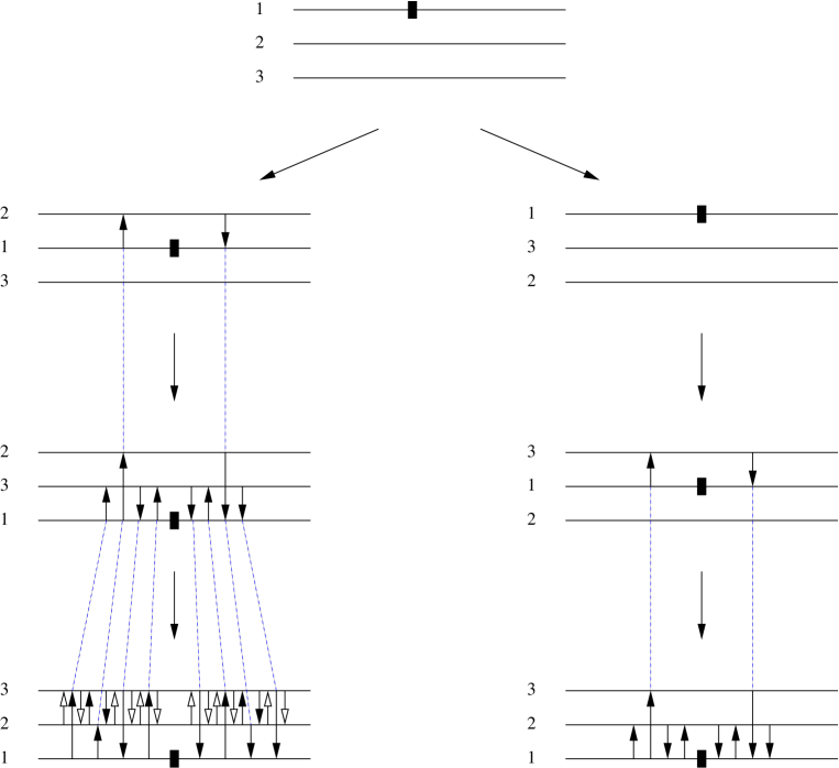
Figure 5: Generalized YBE 1.

The consistency conditions follow from considering the different ways of exchanging the product of three Wilson lines with insertions. We first consider the case of gauge invariant insertions; in this case the R-matrices are c-numbers. Then we will consider the case of non-gauge-invariant insertions, namely loose endpoints. In this case the R-matrices are field-dependent, and the generalized Yang-Baxter equations are of the dynamical type.

8.1 Generalized quantum YBE

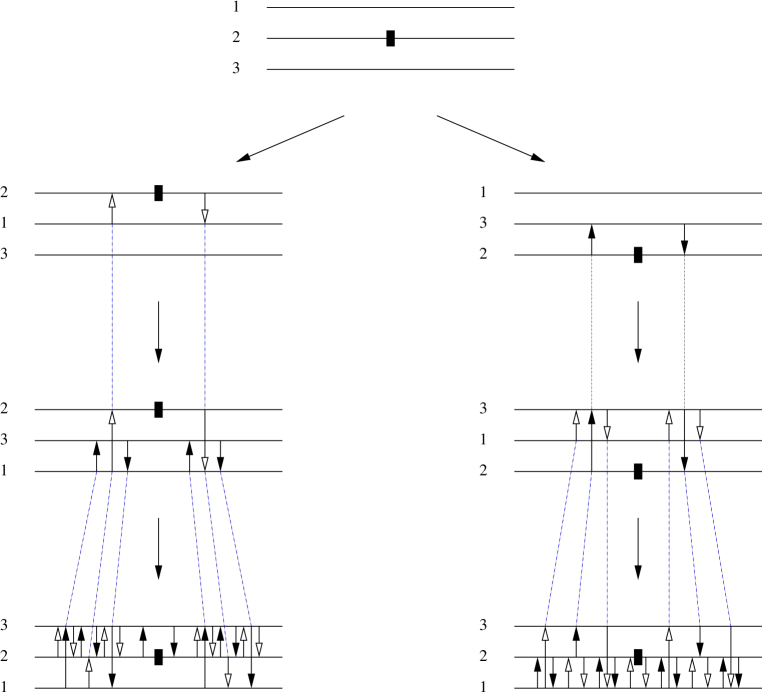
Figure 6: Generalized YBE 2.

To understand the quantum consistency conditions for the $R$ matrices let us put the Wilson line with the spectral parameter switch on top of two other Wilson lines, the other two Wilson lines having no operator insertions. The equations of this section will not change if we put a constant gauge invariant operator at the point on the upper contour where we switch the spectral parameter (instead of just $1$). For example, $C^{\mu\nu}t^{2}_{\mu}t^{2}_{\nu}$ is a constant gauge invariant operator. It is gauge invariant because commutes with $\mathfrak{g}_{\bar{0}}$.

The generalized quantum Yang-Baxter equations (qYBE) are obtained from the exchanges illustrated in figure 5. The notations are: $\;=R_{+}$, $\;=R_{+}^{-1}$, $\;=R_{-}$, $\;=R_{-}^{-1}$. The insertion of the spectral parameter changing operator is marked by a black bar.

Equating LHS and RHS in figure 5 yields

$$R_{23,-}R_{13,+}R_{23,-}^{-1}R_{23,+}R_{12,+}R_{23,+}^{-1}R_{23,-}R_{13,+}^{-1}R_{23,-}^{-1}R_{23,-}R_{13,+}R_{23,-}^{-1}\cong R_{12,+}R_{13,+}R_{12,+}^{-1}R_{12,+}\,.$$ (8.2)

After cancellations of $RR^{-1}$:

$$R_{23,-}R_{13,+}R_{23,-}^{-1}R_{23,+}R_{12,+}R_{23,+}^{-1}\cong R_{12,+}R_{13,+}\,.$$ (8.3)

Here the sign $\cong$ means that the ratio of the left hand side and the right hand side commutes with ${\cal O}$:

$$R_{13,+}^{-1}R_{12,+}^{-1}R_{23,-}R_{13,+}R_{23,-}^{-1}R_{23,+}R_{12,+}R_{23,+}^{-1} = T_{123}$$ (8.4)

$$T_{123}{\cal O}_{1}T_{123}^{-1} = {\cal O}_{1}\,.$$ (8.5)

At the first order of perturbation theory the left hand side of (8.4) is, cf. (2.47) and (2.48),

$$[r_{23,-},r_{13,+}]+[r_{13,+},r_{12,+}]+[r_{23,+},r_{12,+}]\;=$$ (8.6)

And the right hand side of (8.4) is:

$$= -4\;t^{0}\otimes(z_{2}^{2}-z_{2}^{-2})t^{2}\otimes(z_{3}^{2}-z_{3}^{-2})[t^{0},t^{2}]-$$

$$-4\;t^{0}\otimes(z_{2}-z_{2}^{-3})t^{1}\otimes(z_{3}^{3}-z_{3}^{-1})[t^{0},t^{3}]-$$

$$-4\;t^{0}\otimes(z_{2}^{3}-z_{2}^{-1})t^{3}\otimes(z_{3}-z_{3}^{-3})[t^{0},t^{1}]$$

(the indices of $t^{0}$ contract with the indices of another $t^{0}$, so $t^{0}\otimes t^{0}$ stands for $C^{[\mu_{1}\nu_{1}][\mu_{2}\nu_{2}]}\;t^{0}_{[\mu_{1}\nu_{1}]}\otimes t^{0}_{[\mu_{2}\nu_{2}]}$; similarly the indices of $t^{2}$ contract with the indices of another $t^{2}$, and $t^{1}$ with $t^{3}$.) Our ${\cal O}$ is just the spectral parameter switch, it is a constant gauge invariant operator. In particular, $[t^{0},{\cal O}]=0$, cf. (8.5). In other words, eq. (8.6,8.1) is the generalized classical Yang-Baxter equation modulo gauge transformation.

Similarly, putting the switch operator on the lower contour (see Figure 5) we get the following consistency condition:

$$R_{23,+}R_{13,-}R_{23,+}^{-1}R_{23,-}R_{12,-}R_{23,-}^{-1}=R_{12,-}R_{13,-}\,.$$ (8.8)

Finally we turn to the exchange of $R_{+}$ and $R_{-}$, which is derived in Figure 6. Equating the LHS and RHS of this graph, we obtain

$$(R_{23-}R_{13+}R_{23-}^{-1})(R_{23+}R_{12-}R_{23+}^{-1})(R_{23-}R_{13-}^{-1}R_{23-}^{-1})R_{23+}$$ (8.9)

$$= (R_{12+}R_{13-}R_{12+}^{-1})(R_{12-}R_{23+}R_{12-}^{-1})(R_{12+}R_{13-}^{-1}R_{12+}^{-1})R_{12-}\,.$$

Note that we equate of course only one side of the insertion at a time. Note also, that for $R_{+}=R_{-}$ this returns to a standard YBE. Another way of writing it:

$$R_{12-}R_{23+}^{-1}$$ (8.10)

$$=(\hbox{ad}_{R_{12+}}(R_{13-})\hbox{ad}_{R_{12-}}(R_{23+})\hbox{ad}_{R_{12+}}(R_{13-}^{-1}))^{-1}(\hbox{ad}_{R_{23-}}(R_{13+})\hbox{ad}_{R_{23+}}(R_{12-})\hbox{ad}_{R_{23-}}(R_{13-}^{-1}))\,.$$

In [19, 20] another generalization of quantum YBE was proposed as the quantum version of a more restricted set of classical YBE. The main difference to the equations here is that the ones in [19, 20] impose the standard qYBE on $R$ (and thus the standard YBE on the classical $r$-matrix) and supplement these by equations of the type $RSS=SSR$. However the main problem with this approach is that the case of principal chiral models and strings on $AdS_{5}\times S^{5}$ do not fall in the class of models where $r$ satifies the YBE separately from $s$.

8.2 Some speculations on charges

Strictly speaking our derivation of equations like (8.3) only applies to the terms quadratic in $r$ (i.e. tree level). Although the derivation outlined in Figures 5 and 6 seems to apply also at the level of higher loops, in fact there might be subtleties associated to overlapping diagramms involving all three lines.

Nevertheless, let us for a moment take the proposed generalized qYBE (8.3) seriously and see how it could be put to use in order to construct a quadratic algebra of $RTT$ type. The relation (8.3) can be thought of in the following way. Let us begin with the standard YBE, which reads

$$R_{12}R_{13}R_{23}=R_{23}R_{13}R_{12}\,.$$ (8.11)

This can formally be thought of as “$R_{12}$ and $R_{13}$ commute up to conjugation by $R_{23}$”, or explicitly

$$R_{12}R_{13}=\left(R_{23}R_{13}R_{23}^{-1}\right)\left(R_{23}R_{12}R_{23}^{-1}\right)$$ (8.12)

The relation (8.3) generalizes this version of the YBE naturally, in that

$$R_{12,+}R_{13,+}=\left(R_{23,-}R_{13,+}R_{23,-}^{-1}\right)\left(R_{23,+}R_{12,+}R_{23,+}^{-1}\right)\,.$$ (8.13)

If we interpret this as $RTT$ relations, we obtain

$$T_{12,+}T_{13,+}=\left(R_{23,-}T_{13,+}R_{23,-}^{-1}\right)\left(R_{23,+}T_{12,+}R_{23,+}^{-1}\right)\,.$$ (8.14)

Naively one might then conclude that this equation is in fact of the type that has been discussed in [19], equation (14)

$$A_{12}T_{1}B_{12}T_{2}=T_{2}C_{12}T_{1}D_{12}\,,$$ (8.15)

where $T_{1}=T_{12,+}$ and $T_{2}=T_{13,+}$ and

$$A_{12}=R_{23,-}^{-1}\,,\quad B_{12}={\bf 1}\,,\quad C_{12}=R_{23,-}^{-1}R_{23,+}\,,\quad D_{12}=R_{23,+}^{-1}\,.$$ (8.16)

However, in [19] it is required that the matrices $A,B,C,D$ satisfy a set of equations, in particular $A$ and $D$ have to separately satisfy the standard YBE, as well as equations of the type $ACC=CCA$ and $DCC=CCD$ as well as $[A_{12},C_{13}]=0$ and $[D_{12},C_{32}]=0$ have to hold (note that it is pointed out in [19] that these are only sufficient conditions). We do not require these equations, but only seem to be imposing the equation (8.3). This is in fact a much weaker equation, but has the vital advantage that it gives as a classical limit an the algebra of $r-s$-matrices as we require it.

In view of the algebra (8.13) the standard argument of construction of commuting charges does not go through, namely $[\hbox{tr}_{2}(T_{12,+}),\hbox{tr}_{3}(T_{13,+})]$ is not obviously vanishing, as the conjugation in this case is by $R_{23,+}$ and $R_{23,-}$ respectively, which do not agree in the present case. At this point a construction that appears in [19] is useful, despite the fact that their transfer matrix algebra is different from ours. First let us simplify notation and suppress the physical space index of the $T$-matrices, so we consider the exchange relation of $T_{2}$ and $T_{3}$. $T_{i}$ is an element of End$(\rho_{a})\equiv\rho_{a}\otimes\rho_{a}^{\ast}$ (at least for finite dimensional representations). Thus we can label them by $T_{(a,\bar{a})}$, where $\bar{a}$ denotes the dual representation. The generalized RTT relations then become

$$T_{(2,\bar{2})}T_{(3,\bar{3})}=R_{23-}T_{(3,\bar{3})}R_{2\bar{3}-}^{-1}R_{23+}T_{(2,\bar{2})}R_{\bar{2}3+}^{-1}=:{\cal R}_{(3,\bar{3})(2,\bar{2})}T_{(3,\bar{3})}T_{(2,\bar{2})}\,,$$ (8.17)

where $R_{ab}$ acts on the $\rho_{a}$ part of $T_{(a,\bar{a})}$ etc. and we defined

$${\cal R}_{(3,\bar{3})(2,\bar{2})}=R_{23-}R_{2\bar{3}-}^{-1}R_{23+}R_{\bar{2}3+}^{-1}\,.$$ (8.18)

We require that ${\cal R}$ satisfies the YBE, in order for the exchange algebra of $T_{(a,\bar{a})}$ to be consistent. At this point the deviation from the construction in [19] is necessary. Our $R_{ab\pm}$ matrices obey the generalized YBE (8.3) and the complete set of consistency conditions on $R_{\pm}$ should imply YBE for ${\cal R}$. This requires in particular additional relations for $R_{12-}$ and $R_{21-}$. Once the YBE for $\mathcal{R}$ are established, we define the dual RTT algebra as

$$\hat{T}_{(2,\bar{2})}\hat{T}_{(3,\bar{3})}{\cal R}_{(3,\bar{3})(2,\bar{2})}=\hat{T}_{(3,\bar{3})}\hat{T}_{(2,\bar{2})}\,,$$ (8.19)

Consider a matrix representation (scalar matrix) of (8.19) given by $\hat{\tau}_{(2,\bar{2})}$ and $\hat{\tau}_{(3,\bar{3})}$. There is a natural inner product between the representations and their duals, in particular $\hat{\tau}_{a\bar{a}}.T_{a\bar{a}}$. Thus acting with $\hat{\tau}_{2\bar{2}}\hat{\tau}_{3\bar{3}}$ on the generalized YBE in the form (8.17) we obtain

$$(\hat{\tau}_{2\bar{2}}.T_{2\bar{2}})(\hat{\tau}_{3\bar{3}}.T_{3\bar{3}})=(\hat{\tau}_{3\bar{3}}.T_{3\bar{3}})(\hat{\tau}_{2\bar{2}}.T_{2\bar{2}})\,,$$ (8.20)

and thus

$$[(\hat{\tau}_{2\bar{2}}.T_{2\bar{2}}),(\hat{\tau}_{3\bar{3}}.T_{3\bar{3}})]=0\,.$$ (8.21)

This allows for construction of a family of infinite commuting charges by expanding these expressions in powers of the spectral parameter.

8.3 Contours with loose endpoints

The consistency condition for the exchange of contours with endpoints is more complicated. Again, we can compare $(123)\to(213)\to(231)\to(321)$ to $(123)\to(132)\to(312)\to(321)$. When we exchange $(123)\to(213)$ we get the insertion of the split operator ${\cal F}_{-}^{-1}({\cal F}_{+}(1))$:

At the first order of perturbation theory:

$${\cal F}_{-}^{-1}({\cal F}_{+}(1))=\mathfrak{1}+r+s+q\,,$$ (8.22)

where $q$ are field-dependent (= dynamical) terms. Indeed, the main difference between the exchange of the switch operator and the exchange of the endpoint is that the endpoint is not gauge invariant and therefore the exchange matrix is field dependent. The expansion of $q$ in powers of $x$ and $\vartheta$ starts with:

$$q={1\over 2}\left([x,t^{2}]\otimes t^{2}+\{\vartheta^{3},t^{1}\}\otimes t^{3}+\{\vartheta^{1},t^{3}\}\otimes t^{1}\right)+\ldots$$ (8.23)

Then, when we exchange $(213)\to(231)\to(321)$ we get additional contributions coming from the contraction of $q_{12}$ with the currents integrated over line 3, for example:

(8.24)

On the other hand, if we look at the field independent (leading) terms, we will get an equation identical to (8.4), but now $T_{123}$ does not act as the identity on the endpoint, because the endpoint is not gauge invariant. But in fact the $T$ on the right hand side of (8.4) cancels with the terms arising from the contractions (8.24).

To summarize, we have the following two types of consistency conditions:

1. Consistency conditions for the exchange of gauge invariant operators. In this case the right hand side of (8.4) does not spoil the consistency because of equation (8.5), which expresses the gauge invariance of the inserted operators.

2. Consistency conditions for the insertions which are not gauge invariant. In this case the right hand side of (8.4) cancels against the terms arising from the diagrams like (8.24).

9 Conclusions and Discussion

We have setup a formalism in which to compute the product of two transfer matrices, using the operator algebra of the currents. In particular, to leading order in the expansion around flat space-time, a structure reminiscent of classical $r$-matrices appears. This is however modified in that we require a system of $r$ and $s$-matrices, which satisfy a generalized classical YBE. This is related in the approach of [15] to Poisson brackets being non-ultralocal.

We consider it a first step towards constructing the analog of a quantum $R$-matrix, which satisfies a generalized quantum YBE. The situation is different from [19, 20], because the classical $r$-matrix in our case does not satisfy the standard classical YBE (which is one of the assumptions that goes into the construction in [19, 20]) but the combined equation for $r$ and $s$ (8.6).

The most promising direction to extend this work is to construct the quantum conserved charges from the $T$-matrices, as outlined in section 8.2. It would also be interesting to test the generalized quantum YBE explicitly at higher orders in the $1/R$ expansion.

It would also be interesting to understand how the $r$-$s$-matrices found here relate to the classical $\mathfrak{su}(2|2)$ $r$-matrices found from the light-cone string theory and super-Yang Mill dual in [21, 22, 23]. The connection, if it exists, would presumably be along the line of our speculations in section 8.2.

Acknowledgments

We thank Jean-Michel Maillet for very interesting discussions. The research of AM is supported by the Sherman Fairchild Fellowship and in part by the RFBR Grant No. 06-02-17383 and in part by the Russian Grant for the support of the scientific schools NSh-8065.2006.2. The research of SSN is supported by a John A. McCone Postdoctoral Fellowship of Caltech. We thank the Isaac Newton Institute, Cambridge, for generous hospitality during the completion of this work.

Appendix A Calculation of the products of currents

Here we will describe some methods for calculating the singularities in the product of two currents. We will only discuss two examples. The first example is the collision $J_{3+}J_{3+}$ and the collision $J_{1+}J_{2+}$. The second is the singularities proportional to $xdx$ in the collision $J_{2+}J_{2+}$, which we needed in Section 5.2.2.

A.1 Collisions $J_{3+}J_{3+}$ and $J_{1+}J_{2+}$.

Collision $J_{3+}J_{3+}$

$$(\partial_{+}\vartheta_{L}+[\vartheta_{R},\partial_{+}x])^{\alpha}(w_{a}){\bf\longleftrightarrow}(\partial_{+}\vartheta_{L}+[\vartheta_{R},\partial_{+}x])^{\beta}(w_{b})\,.$$ (A.1)

The cubic vertex $([\vartheta_{L},\partial_{-}\vartheta_{L}]\partial_{+}x)$ does not contribute to the singularity, but the other cubic vertex does:

$$-S\mapsto{1\over\pi}\int d^{2}v\;{1\over 2}\mbox{str}\;\left([\vartheta_{R},\partial_{+}\vartheta_{R}]\partial_{-}x\right)\,.$$ (A.2)

After integration by parts the interaction vertex becomes:

$$-{1\over\pi}\int d^{2}v\;{1\over 2}\mbox{str}\;\left([\partial_{-}\vartheta_{R},\partial_{+}\vartheta_{R}]x+\mbox{str}\;[\vartheta_{R},\partial_{+}\partial_{-}\vartheta_{R}]x\right)\,.$$ (A.3)

Integrating by parts $\partial_{+}$ in the second term we get:

$${1\over\pi}\int d^{2}v\;\mbox{str}\;\left(-[\partial_{-}\vartheta_{R},\partial_{+}\vartheta_{R}]x+{1\over 2}\mbox{str}\;[\vartheta_{R},\partial_{-}\vartheta_{R}]\partial_{+}x\right)\,.$$ (A.4)

This implies that (A.1) gives the same singularity as the following collision in the free theory:

$$\left(\partial_{+}\vartheta_{L}-[\partial_{+}\vartheta_{R},x]+{1\over 2}[\vartheta_{R},\partial_{+}x]\right)^{\alpha}(w_{a}){\bf\longleftrightarrow}\left(\partial_{+}\vartheta_{L}-[\partial_{+}\vartheta_{R},x]+{1\over 2}[\vartheta_{R},\partial_{+}x]\right)^{\beta}(w_{b})\,.$$ (A.5)

The singularity is:

$${1\over(w_{a}-w_{b})^{2}}([t^{1},x(w_{a})]\otimes t^{3}+t^{3}\otimes[t^{1},x(w_{b})])+$$

$$+{1\over 2}{1\over w_{a}-w_{b}}([t^{1},\partial_{+}x(w_{a})]\otimes t^{3}-t^{3}\otimes[t^{1},\partial_{+}x(w_{b})])\,.$$ (A.6)

This is equal to:

$${2\over w_{a}-w_{b}}[t^{1},\partial_{+}x]\otimes t^{3}+{\overline{w}_{a}-\overline{w}_{b}\over(w_{a}-w_{b})^{2}}[t^{1},\partial_{-}x]\otimes t^{3}\,.$$ (A.7)

Collision $J_{1+}J_{2+}$

$$(\partial_{+}\vartheta_{R}+[\vartheta_{L},\partial_{+}x]){\bf\longleftrightarrow}(\partial_{+}x+1/2[\vartheta_{L},\partial_{+}\vartheta_{L}]+\ldots)\,.$$ (A.8)

We have to take into account the interaction vertex in the action:

$$-S\mapsto{1\over\pi}\int d^{2}v{1\over 2}\mbox{str}\;\left([\vartheta_{L},\partial_{-}\vartheta_{L}]\partial_{+}x\right)\,.$$ (A.9)

It is convenient to denote the contracted fields by using prime. For example, this notation:

$${1\over 2}\mbox{str}\;\left([\vartheta^{\prime}_{L},\partial_{-}\vartheta_{L}]\partial_{+}x^{\prime}\right)\,.$$ (A.10)

means that ${\vartheta_{L}}$ is contracted with the $\partial_{+}\vartheta_{R}$ in $J_{1+}$, and ${\partial_{+}x}$ with $\partial_{+}x$ in $J_{2+}$. Therefore $\partial_{-}\vartheta_{L}$ remains uncontracted. There is another possible contraction:

$${1\over 2}\mbox{str}\;\left([\vartheta_{L},\partial_{-}\vartheta^{\prime}_{L}]\partial_{+}x^{\prime}\right)\,.$$ (A.11)

In the interaction vertex (A.10) let us integrate by parts $\partial_{-}$. We will get:

$$-{1\over 2}\mbox{str}\left([\partial_{-}\vartheta^{\prime}_{L},\vartheta_{L}]\partial_{+}x^{\prime}\right)-{1\over 2}\mbox{str}\left([\vartheta^{\prime}_{L},\vartheta_{L}]\partial_{-}\partial_{+}x^{\prime}\right)\,.$$ (A.12)

In the second expression let us integrate by parts $\partial_{+}$. The result is:

$$-{1\over 2}\mbox{str}\left([\partial_{-}\vartheta^{\prime}_{L},\vartheta_{L}]\partial_{+}x^{\prime}\right)+{1\over 2}\mbox{str}\left([\partial_{+}\vartheta^{\prime}_{L},\vartheta_{L}]\partial_{-}x^{\prime}\right)+{1\over 2}\mbox{str}\left([\vartheta^{\prime}_{L},\partial_{+}\vartheta_{L}]\partial_{-}x^{\prime}\right)\,.$$ (A.13)

The first term coincides with (A.11), and together with (A.11) gives:

$$-\mbox{str}\left([\partial_{-}\vartheta^{\prime}_{L},\vartheta_{L}]\partial_{+}x^{\prime}\right)\,.$$ (A.14)

This is easy to contract, and precisely cancels the “direct hit” $[\vartheta_{L},\partial_{+}x]{\bf\longleftrightarrow}\partial_{+}x$. The second and thrid terms combine with the “direct hit”

$$\partial_{+}\vartheta_{R}{\bf\longleftrightarrow}1/2[\vartheta_{L},\partial_{+}\vartheta_{L}]$$ (A.15)

to give the same contribution as the collision

$$\partial_{+}\vartheta_{R}^{\prime}{\bf\longleftrightarrow}[\vartheta_{L}^{\prime},\partial_{+}\vartheta_{L}]\,,$$ (A.16)

which gives:

$${\partial_{+}\vartheta_{L}^{\alpha}\over w_{a}-w_{b}}f_{\alpha}{}^{\dot{\alpha}\mu}\,.$$ (A.17)

A.2 Terms $xdx$ in the collision $J_{2+}J_{2+}$

Consider this collision:

  $z^{-2}J_{2+}$    $z^{-2}J_{2+}$ 

More explicitly, we are looking at:

$$\left(\partial_{+}x+{1\over 6}[x,[x,\partial_{+}x]]\right)(w_{u})\stackrel{{\scriptstyle\otimes}}{{\leftrightarrow}}\left(\partial_{+}x+{1\over 6}[x,[x,\partial_{+}x]]\right)(w_{d})\,.$$ (A.18)

Couplings to $xdx$ receive contributions from the quartic interaction vertex:

$$-S\mapsto{1\over 6\pi}\mbox{str}[x,\partial_{+}x][x,\partial_{-}x]\,.$$ (A.19)

We denote the contracted fields $x^{\prime}(w_{u})$ and $x^{\prime\prime}(w_{d})$. When $\partial_{-}x$ in the interaction vertex gets contracted with $\partial_{+}x$ in one of the $J_{2+}$, this contribution cancels the “direct hit” $\partial_{+}x{\bf\longleftrightarrow}{1\over 6}[x,[x,\partial_{+}x]]$. Let us study the diagrams in which $\partial_{-}x$ in the interaction vertex remains uncontracted. There are the following possibilities:

$${1\over 6\pi}\int d^{2}v\;\mbox{str} (2[x^{\prime},\partial_{+}x^{\prime\prime}][x,\partial_{-}x]+$$ (A.22)

$$+[x,\partial_{+}x^{\prime}][x^{\prime\prime},\partial_{-}x]+$$

$$+[x,\partial_{+}x^{\prime\prime}][x^{\prime},\partial_{-}x])\,.$$

Here prime and double prime mark the contracted elementary fields; for example in the first term $2[x^{\prime},\partial_{+}x^{\prime\prime}][x,\partial_{-}x]$ the elementary field $x^{\prime}$ contracts with $\partial_{+}x(w_{u})$ in $z_{u}^{-2}J_{2+}(w_{u})$ and $\partial_{+}x^{\prime\prime}$ contracts with $\partial_{+}x(w_{d})$ in $z_{d}^{-2}J_{2+}(w_{d})$; while $[x,\partial_{-}x]$ remains uncontracted. This gives:

$${1\over 6\pi}\int d^{2}v\;\mbox{str} \left({(-2)\over(v-w_{u})(v-w_{d})^{2}}C^{\mu\nu}[t^{2}_{\mu},[x,\partial_{-}x]]\otimes t_{\nu}^{2}-\right.$$

$$-{(-1)\over(v-w_{u})^{2}(v-w_{d})}C^{\mu\nu}[x,[t^{2}_{\mu},\partial_{-}x]]\otimes t_{\nu}^{2}-$$

$$\left.-{(-1)\over(v-w_{u})(v-w_{d})^{2}}C^{\mu\nu}t^{2}_{\mu}\otimes[x,[t^{2}_{\nu},\partial_{-}x]]\right)=$$

$$= -{1\over 2\pi}\int d^{2}v\;\mbox{str} {1\over(v-w_{u})(v-w_{d})^{2}}C^{\mu\nu}[t^{2}_{\mu},[x,\partial_{-}x]]\otimes t_{\nu}^{2}=$$ (A.24)

$$=-{1\over 2}{\overline{w}_{d}-\overline{w}_{u}\over(w_{d}-w_{u})^{2}}C^{\mu\nu}[t^{2}_{\mu},[x,\partial_{-}x]]\otimes t_{\nu}^{2}\,.$$

(A simple way to get the singularity of this integral is by considering ${\partial\over\partial\overline{w}_{u}}$.) This contributes to the current-generator coupling:

$${1\over 2}\pi i\;C^{\mu\nu}(z^{-2}[t^{2}_{\mu},[x,\partial_{-}x]])\otimes(z^{-2}t^{2}_{\nu})$$ (A.25)

Taking into account that $C^{\mu\nu}[t^{2}_{\mu},t^{0}]\otimes t^{2}_{\nu}=-C^{\mu\nu}t^{2}_{\mu}\otimes[t^{2}_{\nu},t^{0}]$ we can rewrite (A.25) using the $\wedge$-product:

$${1\over 2}\pi i\;C^{\mu\nu}(z^{-2}[t^{2}_{\mu},[x,\partial_{-}x]])\wedge(z^{-2}t^{2}_{\nu})\,.$$

A.3 Short distance singularities using index notations

In the main text we gave the expressions for the short distance singularities in the tensor product notations. Here we list the singularities using more “conservative” index notations:

$$J_{1-}^{\dot{\alpha}}(w_{1})J_{2+}^{\mu}(w_{2}) = {1\over R^{3}}{\partial_{-}\vartheta_{L}^{\gamma}\over w_{1}-w_{2}}f_{\gamma}{}^{\dot{\alpha}\mu}$$ (A.26)

$$J_{1+}^{\dot{\alpha}}(w_{1})J_{2-}^{\mu}(w_{2}) = {1\over R^{3}}{\partial_{-}\vartheta^{\gamma}_{L}\over w_{1}-w_{2}}f_{\gamma}{}^{\dot{\alpha}\mu}$$ (A.27)

$$J_{3-}^{\alpha}(w_{1})J_{2+}^{\mu}(w_{2}) = {1\over R^{3}}{\partial_{+}\vartheta^{\dot{\gamma}}_{R}\over\bar{w}_{1}-\bar{w}_{2}}f_{\dot{\gamma}}{}^{\dot{\alpha}\mu}$$ (A.28)

$$J_{3+}^{\alpha}(w_{1})J_{2-}^{\mu}(w_{2}) = {1\over R^{3}}{\partial_{+}\vartheta^{\dot{\gamma}}_{R}\over\bar{w}_{1}-\bar{w}_{2}}f_{\dot{\gamma}}{}^{\alpha\mu}$$ (A.29)

$$J_{1+}^{\dot{\alpha}}(w)J_{1-}^{\dot{\beta}}(0) = -{1\over R^{3}}{\partial_{-}x^{\mu}\over w_{a}-w_{b}}f_{\mu}{}^{\dot{\alpha}\dot{\beta}}$$ (A.30)

$$J_{3+}^{\alpha}(w)J_{3-}^{\beta}(0) = -{1\over R^{3}}{\partial_{+}x^{\mu}\over\bar{w}_{a}-\bar{w}_{b}}f_{\mu}{}^{\alpha\beta}$$ (A.31)

$$J_{1+}^{\dot{\alpha}}(w_{1})J_{2+}^{\mu}(w_{2}) = {1\over R^{3}}{\partial_{+}\vartheta_{L}^{\gamma}\over w_{1}-w_{2}}f_{\gamma}{}^{\dot{\alpha}\mu}+O\left({1\over R^{4}}\right)$$ (A.32)

$$J_{3+}^{\alpha}(w_{3})J_{2+}^{\mu}(w_{2}) = {2\over R^{3}}{\partial_{+}\vartheta_{R}^{\dot{\beta}}\over w_{3}-w_{2}}f_{\dot{\beta}}{}^{\alpha\mu}+{1\over R^{3}}{\bar{w}_{3}-\bar{w}_{2}\over(w_{3}-w_{2})^{2}}\partial_{-}\vartheta_{R}^{\dot{\gamma}}f_{\dot{\gamma}}{}^{\alpha\mu}+O\left({1\over R^{4}}\right)$$ (A.33)

$$J_{1+}^{\dot{\alpha}}(w_{a})J_{1+}^{\dot{\beta}}(w_{b}) = -{1\over R^{3}}{\partial_{+}x^{\mu}\over w_{a}-w_{b}}f_{\mu}{}^{\dot{\alpha}\dot{\beta}}+O\left({1\over R^{4}}\right)$$ (A.34)

$$J_{3+}^{\alpha}(w_{a})J_{3+}^{\beta}(w_{b}) = -{2\over R^{3}}{\partial_{+}x^{\mu}\over w_{a}-w_{b}}f_{\mu}{}^{\alpha\beta}-{1\over R^{3}}{\bar{w}_{a}-\bar{w}_{b}\over(w_{a}-w_{b})^{2}}\partial_{-}x^{\mu}f_{\mu}{}^{\alpha\beta}+O\left({1\over R^{4}}\right)$$ (A.35)

$$J_{1+}^{\dot{\alpha}}(w_{1})J_{3+}^{\alpha}(w_{3}) = -{1\over R^{2}}{1\over(w_{1}-w_{3})^{2}}C^{\dot{\alpha}\alpha}+O\left({1\over R^{4}}\right)$$ (A.36)

$$J_{2+}^{\mu}(w_{m})J_{2+}^{\nu}(w_{n}) = -{1\over R^{2}}{1\over(w_{m}-w_{n})^{2}}C^{\mu\nu}+O\left({1\over R^{4}}\right)$$ (A.37)

$$J_{0+}^{[\mu\nu]}(w_{0})J_{1+}^{\dot{\alpha}}(w_{1}) = -{1\over 2R^{3}}\left({\vartheta_{R}^{\dot{\beta}}(w_{0})\over(w_{0}-w_{1})^{2}}+{\partial_{+}\vartheta_{R}^{\dot{\beta}}(w_{0})\over(w_{0}-w_{1})}\right)f_{\dot{\beta}}{}^{\dot{\alpha}[\mu\nu]}+O\left({1\over R^{4}}\right)$$ (A.38)

$$J_{0+}^{[\mu\nu]}(w_{0})J_{3+}^{\alpha}(w_{3}) = -{1\over 2R^{3}}\left({\vartheta_{L}^{\beta}(w_{0})\over(w_{0}-w_{3})^{2}}+{\partial_{+}\vartheta_{L}^{\beta}(w_{0})\over(w_{0}-w_{3})}\right)f_{\beta}{}^{\alpha[\mu\nu]}+O\left({1\over R^{4}}\right)$$ (A.39)

$$J_{0+}^{[\mu\nu]}(w_{0})J_{2+}^{\lambda}(w_{2}) = -{1\over 2R^{3}}\left({x^{\kappa}(w_{0})\over(w_{0}-w_{2})^{2}}+{\partial_{+}x^{\kappa}(w_{0})\over(w_{0}-w_{2})}\right)f_{\kappa}{}^{\lambda[\mu\nu]}+O\left({1\over R^{4}}\right)\,.$$ (A.40)

Appendix B Very brief summary of the Maillet formalism

Let us briefly review the situation in Maillet et al’s work and how this connects to our present analysis. In [15] a formalism was developed which generalizes the classical YBE to incorporate the case of non-ultralocal Poisson brackets. Consider the algebra of $L$-matrices (spatial component of the Lax operator)

$$\{L(\sigma_{1},z_{1}),L(\sigma_{2},z_{2})\} =[r(\sigma_{1},z_{1},z_{2}),\mathfrak{1}\otimes L(\sigma_{1},z_{1})+L(\sigma_{1},z_{1})\otimes\mathfrak{1}]\delta(\sigma_{1}-\sigma_{2})$$ (B.1)

$$+[s(\sigma_{1},z_{1},z_{2}),\mathfrak{1}\otimes L(\sigma_{1},z_{1})-L(\sigma_{1},z_{1})\otimes\mathfrak{1}]\delta(\sigma_{1}-\sigma_{2})$$

$$-\left(s(\sigma_{1},z_{1},z_{2})+s(\sigma_{2},z_{1},z_{2})\right)\delta^{\prime}(\sigma_{1}-\sigma_{2})\,.$$

The terms proportional to $\delta^{\prime}$ are the so-called non-ultralocal terms. The algebra (B.1) is a deformation of the standard ultra-local one by terms depending on the matrix $s$, which unlike $r$ is symmetric. Jacobi-identity for $\{,\}$ yields a generalized, dyamical YBE

$$[r_{12}-s_{12},r_{13}+s_{13}]+[r_{12}+s_{12},r_{23}+s_{23}]+[r_{13}+s_{13},r_{23}+s_{23}]+H_{1,23}^{(r+s)}-H_{2,13}^{(r+s)}=0\,.$$ (B.2)

The dynamicity is due to the terms $H_{i,jk}$, which arise if $r+s$ is field dependent and are defined by

$$\{L(\sigma_{1},z_{1})\otimes\mathfrak{1}\otimes\mathfrak{1},\mathfrak{1}\otimes(r+s)_{23}(\sigma_{2},z_{2},z_{3})\}=H_{1,23}^{(r+s)}(\sigma_{1},z_{1},z_{2},z_{3})\delta(\sigma_{1}-\sigma_{2})\,.$$ (B.3)

In the case of $s=0$ and $r$ constant (field-independent) the relation (B.2) reduces to the standard classical YBE. This formulation was applied to the $O(n)$ model [15] and the complex Sine-Gordon model [14] (where in both cases the $r-s$-matrices are dynamical), as well as the principal chiral field [13], in which case the terms $H_{i,jk}$ vanish. Note that the field-dependence of the $r-s$-matrices seems to be due to the field-dependence of the non-ultralocal term.

Bibliography

- [1] N. Beisert, R. Hernandez, and E. Lopez, A crossing-symmetric phase for AdS(5) x S(5) strings, JHEP 11 (2006) 070, [hep-th/0609044].
- [2] N. Beisert, B. Eden, and M. Staudacher, Transcendentality and crossing, J. Stat. Mech. 0701 (2007) P021, [hep-th/0610251].
- [3] V. V. Bazhanov, S. L. Lukyanov, and A. B. Zamolodchikov, Integrable structure of conformal field theory. III: The Yang-Baxter relation, Commun. Math. Phys. 200 (1999) 297–324, [hep-th/9805008].
- [4] C. Bachas and M. Gaberdiel, Loop operators and the Kondo problem, JHEP 11 (2004) 065, [hep-th/0411067].
- [5] A. Alekseev and S. Monnier, Quantization of Wilson loops in Wess-Zumino-Witten models, hep-th/0702174.
- [6] A. Mikhailov and S. Schafer-Nameki, Perturbative study of the transfer matrix on the string worldsheet in AdS(5) x S(5), arXiv:0706.1525 [hep-th].
- [7] A. Das, J. Maharana, A. Melikyan, and M. Sato, The algebra of transition matrices for the AdS(5) x S(5) superstring, JHEP 12 (2004) 055, [hep-th/0411200].
- [8] A. Das, A. Melikyan, and M. Sato, The algebra of flat currents for the string on AdS(5) x S(5) in the light-cone gauge, JHEP 11 (2005) 015, [hep-th/0508183].
- [9] M. Bianchi and J. Kluson, Current algebra of the pure spinor superstring in AdS(5) x S(5), JHEP 08 (2006) 030, [hep-th/0606188].
- [10] N. Dorey and B. Vicedo, A symplectic structure for string theory on integrable backgrounds, JHEP 03 (2007) 045, [hep-th/0606287].
- [11] A. Mikhailov, Bihamiltonian structure of the classical superstring in AdS(5) x S(5), hep-th/0609108.
- [12] J. Kluson, Reduced sigma-model on O(N): Hamiltonian analysis and Poisson bracket of Lax connection, JHEP 09 (2007) 100, [arXiv:0707.3264 [hep-th]].
- [13] J. M. Maillet, Hamiltonian structures for integrable classical theories from graded Kac-Moody algebras, Phys. Lett. B167 (1986) 401.
- [14] J. M. Maillet, New integrable canonical structures in two-dimensional models, Nucl. Phys. B269 (1986) 54.
- [15] J. M. Maillet, Kac-Moody algebra and extended Yang-Baxter relations in the O(N) nonlinear sigma model, Phys. Lett. B162 (1985) 137.
- [16] J. Kluson, Note about classical dynamics of pure spinor string on AdS(5) x S(5) background, Eur. Phys. J. C50 (2007) 1019–1030, [hep-th/0603228].
- [17] A. A. Rosly and K. G. Selivanov, On amplitudes in self-dual sector of Yang-Mills theory, Phys. Lett. B399 (1997) 135–140, [hep-th/9611101].
- [18] V. G. M. Puletti, Operator product expansion for pure spinor superstring on AdS(5) x S(5), JHEP 10 (2006) 057, [hep-th/0607076].
- [19] L. Freidel and J. M. Maillet, Quadratic algebras and integrable systems, Phys. Lett. B262 (1991) 278–284.
- [20] L. Freidel and J. M. Maillet, On classical and quantum integrable field theories associated to Kac-Moody current algebras, Phys. Lett. B263 (1991) 403–410.
- [21] A. Torrielli, Classical r-matrix of the su(2—2) SYM spin-chain, Phys. Rev. D 75, 105020 (2007) hep-th/0701281.
- [22] S. Moriyama and A. Torrielli, A Yangian Double for the AdS/CFT Classical r-matrix, JHEP 0706, 083 (2007) arXiv:0706.0884 [hep-th].
- [23] N. Beisert and F. Spill, The Classical r-matrix of AdS/CFT and its Lie Bialgebra Structure, arXiv:0708.1762 [hep-th].