3D Distribution of Molecular Gas in the Barred Milky Way

Abstract

We present a new model of the three-dimensional distribution of molecular gas in the Milky Way Galaxy, based on CO line data.

Our analysis is based on a gas-flow simulation of the inner Galaxy using smoothed-particle hydrodynamics (SPH) using a realistic barred gravitional potential derived from the observed COBE/DIRBE near-IR light distribution. The gas model prescribes the gas orbits much better than a simple circular rotation model and is highly constrained by observations, but it cannot predict local details. In this study, we provide a 3D map of the observed molecular gas distribution using the velocity field from the SPH model. A comparison with studies of the Galactic Center region suggests that the main structures are reproduced but somewhat stretched along the line-of-sight, probably on account of limited resolution of the underlying SPH simulation. The gas model will be publicly available and may prove useful in a number of applications, among them the analysis of diffuse gamma-ray emission as measured with GLAST.

1 Why another deconvolution of gas data?

Models of the distribution of interstellar gas reflect the structure of the Milky Way Galaxy and have therefore considerable merit in themselves. In addition, they are also highly valuable for a variety of other applications, among them the physical analysis of diffuse Galactic gamma-ray emission (Bertsch et al., 1993; Hunter et al., 1997; Pohl & Esposito, 1998). Knowledge of the gas distribution is essential for studies of the large-scale cosmic-ray distribution in the Galaxy, as well as for investigations of small-scale variations in the density and spectrum of cosmic rays. The upcoming launch of GLAST, a GeV-band gamma-ray observatory of unprecedented sensitivity, makes it desirable to have an up-to-date model of the three-dimensional distribution of the ISM. There are two main reasons why a new study would be required: The various components of interstellar gas are traced by their line emission, and the quality of the line data available today is much higher than it was in the Nineties. Also, it is now well established that the Galaxy contains a central bar (e.g. Babusiaux & Gilmore, 2005; Benjamin et al., 2005), which causes non-circular motion of interstellar gas in the inner Galaxy, thus changing the kinematic relation between the location on the line-of-sight and the velocity relative to the local standard of rest (LSR).

Here we report results for the deconvolution of CO_1→0 data for the entire Galactic plane (Dame et al., 2001). For that purpose we use a gas-flow model derived from smoothed particle hydrodynamics (SPH) simulations in gravitational potentials based on the NIR luminosity distribution of the bulge and disk (Bissantz et al., 2003). Besides providing a more accurate picture of cloud orbits in the inner Galaxy, a fundamental advantage of this model is that it provides kinematic resolution toward the Galactic Center, in contrast to standard deconvolution techniques based on purely circular rotation (Nakanishi & Sofue, 2006). Sawada et al. (2004) used OH-absorption data in comparison with CO emission lines to infer the distribution of molecular gas in the inner few hundred parsecs, and found it strongly influenced by the bar. Our model should incorporate the imprint of the bar over the entire inner Galaxy. Therefore, our result does not suffer from a strong finger-of-god effect like in the classical paper by Oort et al. (1958).

Because any deconvolution will introduce artefacts, we test our procedure on simulated line spectra, which allows us to identify artefacts that are present in the final gas model. We investigate three different gas-flow models for the inner Galaxy, one of which is intentionally distorted so it no longer corresponds to a SPH simulation that has been adapted to gas data.

In the Galactic-Center region, for which studies with alternative methods like OH absorption have been performed, we find the gas distribution in our model generally consistent with those earlier results, provided one accounts for the existence of barred gravitational potential. On account of limited resolution both in the gas flow model and the deconvolution the central molecular zone appears somewhat stretched along the line-of-sight, though.

2 The method

2.1 The CO data

The CO_1→0 emission line is the best available tracer of molecular gas, even though the exact relation between the integrated line intensity and the column density of molecular gas, usually referred to as the X-factor, is known to vary with Galactocentric radius and metallicity (Sodroski et al., 1995; Arimoto et al., 1996; Oka et al., 1998; Strong et al., 2004; Nakagawa et al., 2007). The X-factor can be determined at specific locations through the line signal of CO with rare isotopes of either carbon or oxygen using various assumptions for the radiation transport (Dickman, 1978; Dahmen et al., 1998; Wall, 2006) or through absorption measurements of H₂ and CO in the UV (Burgh et al., 2007).

We use the composite survey of Dame et al. (2001), which comprises more than 30 individual surveys of CO_1→0 emission that together cover the entire Galactic Plane. The data were taken with the CfA 1.2-m telescope and a similar instrument in Chile. The angular resolution is about 1/6 of a degree, and the sampling is slightly better than that with 1/8 of a degree. The velocity sampling is 1.3 km/s and the rms noise is around 0.3 K per channel, but varies slightly over the Galactic Plane. The advantage of this survey lies in its sensitivity, the sampling, and the uniformity.

CO surveys have been conducted with significantly higher angular resolution, for example the FCRAO Outer Galaxy Survey (Heyer et al., 1998), the Massachusetts-Stony Brook Galactic Plane CO Survey (Clemens et al., 1986), or the NANTEN Galactic Plane Survey. These surveys either cover only a small part of the sky or are significantly undersampled, thus somewhat compromising their applicability in studies of the large-scale distribution of molecular gas in the Galaxy. Also, considering the width of the point-spread function and the photon statistics at high energies, the effective angular resolution of GLAST is not better than that of the CfA survey, and thus CO data of higher angular resolution may not be needed. We have therefore decided to solely use the CfA survey with a sampling of 1/8 of a degree. By applying the appropriate smoothing we have verified, that the publicly available high-resolution surveys are perfectly consistent with the lower-resolution CfA survey, so by using the CfA survey we have not lost any significant information other than the detailed distribution on scales below 1/6 of a degree.

2.2 The Galactic bar

While bars were clearly observed in other galaxies, absorption of visible light by dust has for a long time impeded searches for similar structures in our Galaxy. The availability of sensitive infrared detectors in recent decades has finally permitted increasingly accurate studies of the structure of inner Galaxy. Today, the observational evidence for the existence of a Galactic bar is very strong (Gerhard, 2001), but some uncertainty remains concerning the characteristics of that bar. As an example, using Spitzer data Benjamin et al. (2005) find a bar with half-length of $R_{\rm bar}\simeq 4$ kpc (for a GC distance of 8 kpc) at an angle of $\phi\simeq 45^{\circ}$, whereas the NIR photometry data of Babusiaux & Gilmore (2005) suggest $R_{\rm bar}\simeq 2.5$ kpc and $\phi\simeq 22^{\circ}$. Using COBE/DIRBE L-band data and giant-star counts Bissantz & Gerhard (2002) determine the bar to be oriented at an angle $\phi\simeq 23^{\circ}$ with spiral arms emerging at $R=3.5$ kpc.

Based on their earlier analysis of the COBE L-band data (Bissantz et al., 1997), Englmaier & Gerhard (1999) have calculated the resulting gravitational potential and modelled the gas flow for the Milky Way inside the solar circle using smoothed particles hydrodynamics in those potentials. It is worth noting, that this model is non-parametric and has virtually no free parameters, except the bar orientation is not tightly constrained by the observations of NIR-light, the microlensing event rate, the red clump giant distribution, and the CO kinematics. Later, in a refined analysis, also the spiral arm pattern was taken into account (Bissantz et al., 2003). To select the best fitting models of the gas flow, Bissantz et al. (2003) compared simulated longitude-velocity diagrams with the main features of observed CO emission for a certain range in Galactic longitude.

Here we use the velocity field from their gas flow models instead of a simple circular rotation curve to determine a distance-velocity relation that will allow us to find the location of molecular gas as traced by CO_1→0 line emission. It is important to note that the non-circular flows imposed by the bar provide kinematic resolution even toward the Galactic Center on account of the radial motion of gas. We use three different velocity-field models in this work. The first is the standard model of Bissantz et al. (2003), which is based on a bar inclination angle $\phi=20^{\circ}$. As alternative we test a model with $\phi=30^{\circ}$ that, according to Bissantz et al. (2003), can also reproduce the main features in position-velocity diagrams of CO line data. The third model is the standard model rotated by $20^{\circ}$, so the bar would make an angle of $\phi=40^{\circ}$ to the line-of-sight and line-of-sight velocities are no longer in accord with the observed velocities of gas. The purpose of that third model is to show the effect of an ill-fitting gas-flow model, and the deduced gas distribution in the Galaxy should be seriously distorted in this case.

Fig. 1 shows the line-of-sight velocity for the standard flow model as a function of distance toward the Galactic Center. For comparison, Fig. 2 gives the CO line spectrum for the same line-of-sight. For the bulk of the line signal at velocities around 50 km/s we now find two possible distance solutions, one near 8 kpc and the other one close to 10 kpc. To be noted from Fig. 1 is also that for many velocities we find a multitude of possible distances, e.g. eight different solutions near zero velocity for the line-of-sight toward the Galactic Center, not just two as in the case of purely circular rotation. Also, the gas flow model does not fully cover the observed range of velocities, as the spectrum in Fig. 2 shows a line signal of about 1 K at -150 km/s and of 2 K at 160 km/s, which is far beyond the range of velocities for which distance solutions exist.

Figure 1: The line-of-sight velocity of interstellar gas as a function of distance for the Galactic Center direction, based on the standard gas flow model of Bissantz et al. (2003). The model successfully predicts large radial velocities, but offers a large variety of possible distance solutions near zero velocity.

Figure 2: The CO_1→0 line spectrum for the Galactic Center direction as given by the CfA data cube. For most of the line signal distances can be found, but some intensity at forbidden velocities remains.

2.3 Deconvolution technique

Many quantities are practically expressed in galactocentric cylinder coordinates $(r,\phi,z)$, but transformations are easier to follow in galactocentric Cartesian coordinates $\vec{r}$. In those coordinates any location is described by a vector $\vec{r}=(r\,\cos\phi,r\,\sin\phi,z)$, and the sun is located at $\vec{r}_{s}=(R_{0},0,z_{0})$, where (e.g. Joshi, 2007)

$$R_{0}=8\ {\rm kpc}\qquad\qquad z_{0}=15\ {\rm pc}$$ (1)

Let us write the distance vector $\vec{y}=\vec{r}-\vec{r}_{s}$ in the form

$$\vec{y}=(-D\,\cos l\,\cos b,-D\,\sin l\,\cos b,D\,\sin b)=(-P\,\cos l,-P\,\sin l,Q)\$$ (2)

where we used heliocentric Galactic coordinates, $D$ is the true distance, and $P$ is the distance as projected on the Galactic plane. For a given CO line spectrum we know the direction in Galactic coordinates $l$,$b$ and can relate $r$ to the line-of-sight velocity. The solution for $P$ then is

$$P = R_{0}\,\cos l+\sqrt{r^{2}-R_{0}^{2}\,\sin^{2}l}\qquad\qquad r\geq R_{0}$$ (3)

$$P = R_{0}\,\cos l\pm\sqrt{r^{2}-R_{0}^{2}\,\sin^{2}l}\qquad\qquad r\leq R_{0}$$ (4)

where always

$$r\geq R_{0}\,|\sin l|$$ (5)

and also

$$D\,\cos b=P\qquad\qquad z=z_{0}+P\,\tan b$$ (6)

Throughout this paper we assume that the gas flow in the Galaxy is independent of $z$, so the flow pattern known for the mid-plane also applies at any height above the plane. This approximation should not cause much error because molecular gas is usually found close to the mid-plane. This assumption holds when $|z|<<r$, i.e. it breaks down very close to the Galactic Center.

If we had a purely circular gas flow with rotation curve $V(r)$, then the uncorrected radial velocity would be

$$V_{\rm LSR}(l,b,P)=\left({{R_{0}}\over r}\,V(r)-V(R_{0})\right)\,\sin l\,\cos b$$ (7)

where Eq. 4 is used to link the projected distance $P$ to the Galactocentric radius $r$. The proper motion of the sun relative to the local standard of rest has a line-of-sight component of (Dehnen & Binney, 1998)

$$V_{\rm LSR,\odot}=\left(10.\,\cos l\,\cos b+5.2\,\sin l\,\cos b+7.2\,\sin b\right)\ {\rm km\,s^{-1}}$$ (8)

which we can account for by subtracting it from the radial velocity. The corrected, effective velocity then is

$$V_{\rm eff}(l,b,P)=V_{\rm LSR}(l,b)-V_{\rm LSR,\odot}$$ (9)

We use Eqs. 7 and 9 to estimate the gas velocity for all Galactocentric radii larger than $R_{0}$, i.e. outside the solar circle, where the gas orbits are assumed circular with constant velocity $V=V_{0}=210$ km/s. The actual rotation velocity of gas in the outer Galaxy depends somewhat on the choice of $R_{0}$, the distance to the Galactic Center. A flat rotation curve with $V_{0}=210$ km/s is a reasonable compromise between faster rotation for larger $R_{0}$ (Levine et al., 2006; McClure-Griffiths & Dickey, 2007) and slower rotation for small $R_{0}$ (Olling & Merrifield, 1998). Inside the solar circle we need to allow for non-circular rotation and therefore the gas velocities are given by the flow model described in subsection 2.2. A linear transition is used to match the gas flow model for the inner and outer Galaxy between 7 kpc and 9 kpc in Galactocentric radius. The flow model of Bissantz et al. (2003) also has a few small data holes that are patched by linear interpolation.

While the bar model provides kinematic resolution toward the Galactic Center, we still face a lack of resolution in the direction of the anticenter, because purely circular rotation is assumed to apply for $r>R_{0}$. Therefore the rotation curve is used only for $|b|\leq 5^{\circ}$ and $|l|\leq 165^{\circ}$. Towards the anticenter, where the kinematic resolution vanishes, we interpolate the distribution of gas between those derived in 10-degree windows centered on $l=160^{\circ}$ and $l=200^{\circ}$ and use that as a probability function according to which the actually measured line signal is distributed. At high latitudes ($|b|\geq 5^{\circ}$) the signal is distributed according to the distance distribution derived for $|b|\leq 5^{\circ}$ as a prior, weighted by a Gaussian of the height above the mid-plane, $z$, for the distance and latitude in question.

The final data cube of deconvolved molecular gas will give the gas density in bins of 100 pc length for the line-of-sight distance, assuming a nominal X-factor $X={2.3\cdot 10^{20}\ \rm mol./cm^{2}/K/(km\,s^{-1})}$. The actual deconvolution uses distance bins of 50 pc length, though, and follows an iterative procedure. The internal velocity dispersion of individual gas clouds is determined from the profiles of narrow lines as

$$\sigma_{\rm CO}=3\ {\rm km/s}$$ (10)

This single-cloud velocity dispersion is small, but still well in the range of those derived in other studies (e.g. Malhotra, 1994). In the Galactic-Center region the velocity dispersion is expected to be higher than that (Dahmen et al., 1998). Within the central kiloparsec we therefore use

$$\sigma_{\rm CO}(r\leq 1\ {\rm kpc})=5\ {\rm km/s}$$ (11)

The actual deconvolution consists of many steps, each of which is supposed to involve an individual gas cloud or part thereof. For that purpose the CO line spectrum is convolved with a Gaussian with half the velocity dispersion of individual gas clouds. The value and velocity of the peak in the convolved spectrum is determined, which is less influenced by noise than if determined through the raw spectrum. Tests have shown that the deconvolution tends to break the total line signal into a few blobs on the line-of-sight, if we place the full peak line signal at the distance corresponding to its velocity, so an iterative process is required. Providing both good computational speed and accuracy, a Gaussian with 20% of that peak value (or the remaining velocity-integrated intensity, whichever is smaller) and a dispersion as given by Eqs. 10 or 11, i.e.

$$I(v)={{\delta W_{\rm CO}}\over{\sqrt{2\pi}\,\sigma_{\rm CO}}}\,\exp\left[-{{(v-v_{0})^{2}}\over{2\,\sigma_{\rm CO}^{2}}}\right]\ ,$$ (12)

is subtracted from the original spectrum and the corresponding $\delta W_{\rm CO}$ value is added to the vector that represents the density distribution along the line-of-sight, thus ensuring that negative fluctuations are not propagated to the density distribution. This procedure is repeated until the velocity-integrated intensity in the remaining CO line spectrum is less than a specified value, here $1\ {\rm K\,km\,s^{-1}}$. The line spectrum that remains when the deconvolution has terminated should contain only noise. Figure 3 shows for a specific line-of-sight the original CO line spectrum in comparison with the convolved spectrum, that is used to find the true peak velocity, and the remaining line spectrum at the end of the deconvolution. To be noted from the figure is that the remaining spectrum does indeed appear to be essentially noise. In the present case the remaining integrated line signal is $0.94\ {\rm K\,km\,s^{-1}}$. It is possible that some of that remaining signal is true emission, and more sensitive observations of the outer Galaxy have in fact found CO line emission at lower level (Nakagawa et al., 2007), but here we have no information as to the velocity (and hence the distance) that this emission should be attributed to. This translates to a systematic uncertainty in the reconstructed column density of molecular gas that can be estimated as

$$\Delta N_{H_{2}}=X\,\Delta W_{\rm CO}\simeq 4\cdot 10^{20}\ {\rm atoms\,cm^{-2}}$$ (13)

for a standard X-factor. Only at high latitude, where the gas column density is low, will this uncertainty have significance compared with uncertainties in the X-factor, limited coverage, or measurement uncertainties. In terms of Galactic diffuse $\gamma$-ray emission above 100 MeV the associated uncertainty is 30% of the extragalactic diffuse background as measured with EGRET (Sreekumar et al., 1998).

Figure 3: The CO_1→0 line spectrum in the direction $l=340^{\circ}$ and $b=0^{\circ}$ at different stages of the deconvolution. The top panel gives the original spectrum as reported by Dame et al. (2001). The middle panel shows that spectrum after convolution with a Gaussian, which we use find the intensity and velocity of the peak emission, assuming true emission lines are significantly broader than the velocity bins of the CO spectrum. The bottom panel displays the remaining spectrum after termination of the deconvolution, which ideally should contain only noise. The residual spectrum shown in the bottom panel is typical. If the velocity dispersion (Eq. 10) were chosen too large, negative spikes could appear that arise from over-subtraction of line wings.

In each iteration step we determine the 8 kinematically best-fitting locations using distance bins of 50 pc length to account for the multitude of possible distance solutions. The line signal is distributed among these eight solutions with weights that are determined by three factors: first a Gaussian function in the separation from the midplane,

$$w_{z}=\exp\left(-{{(z-z_{c})^{2}}\over{2\,\sigma_{z}^{2}}}\right)\ ,$$ (14)

then a Gaussian function with a HWHM of 8.3 kpc in Galactocentric radius to limit the placing of gas at large radii on the far side of the Galaxy, which is often kinematically allowed, but unlikely. The last factors reflects the Jacobian $|dv/dD|$ that arises from transforming a differential in velocity into a differential in line-of-sight distance, $D$. In that Jacobian we have to account for the binning in both velocity and distance. The data cube of the CO line spectrum provides us with the average intensity per velocity interval $\delta v=1.3$ km/s. The Jacobian translates this into an associated distance interval $\Delta_{v}D$, over which the line signal should be distributed,

$$\Delta_{v}D=\bigg{|}{{dv}\over{dD}}\bigg{|}^{-1}\,\delta v\ .$$ (15)

The distance itself is binned with $\delta D=50$ pc. If $\Delta_{v}D\geq\delta D$, which is the standard case, then the signal must be distributed over neighboring bins, each of which receives a fraction $\delta D/\Delta_{v}D$ of the total signal. Our accounting for 8 possible distance solutions at each iteration step together with the usually large number of iteration steps ensures that in this case part of the line signal is indeed attributed to the neighboring distance bins. If $\Delta_{v}D\leq\delta D$, then the signal must nevertheless be distributed over the entire distance bin. In total we can define weight factors representing the Jacobian as

$$w_{J}={{\delta v}\over{\delta D}}\,\cdot\,\cases{1\qquad&{\rm for}\ $\Delta_{v}D\leq\delta D$\cr&\cr{{\delta D}\over{\Delta_{v}D}}&{\rm for}\ $\Delta_{v}D\geq\delta D$}$$ (16)

Gas with forbidden velocity is placed in the distance bins with the best matching velocity, except toward the inner Galaxy ($|l|\leq 20^{\circ}$) where for a velocity offset of more than 10 km/s to the nearest allowed velocity we accept only distance bins in the Galactic Center region. Finally the line-of-sight distribution of gas is reduced to a resolution of 100 pc.

In Eq. 14 we must account for an increase in the thickness of the gas disk with Galactocentric radius. While the variations of $\sigma_{z}$ appear small within the solar circle (Malhotra, 1994; Nakanishi & Sofue, 2006), a substantial flaring of the molecular gas disk is observed in the outer Galaxy (Wouterloot et al., 1990; Binney & Merrifield, 1998). An analytical approximation to the various results reported in the literature is given by

$$\sigma_{z}=60-50\,{r\over{R_{0}}}+60\,\left({r\over{R_{0}}}\right)^{2}\ {\rm pc}$$ (17)

Warping of the molecular disk appears insignificant within the solar circle (Malhotra, 1994; Nakanishi & Sofue, 2006), and therefore we neglect it altogether. In the outer regions of the Galaxy the warp in the molecular disk is assumed identical to that of the H$I$ disk and is given in good approximation by (Binney & Merrifield, 1998)

$$z_{c}=(1,000\,{\rm pc})\,x\,\sin\phi+(300\,{\rm pc})\,x^{2}\,(1-\cos(2\,\phi))$$ (18)

where

$$x={{r-(11\,{\rm kpc})}\over{6\,{\rm kpc}}}\quad{\rm and}\ r\geq 11\,{\rm kpc}$$

Finally, to somewhat alleviate the near-far ambiguity toward the inner Galaxy, we first deconvolve the spectra for Galactic latitudes $|b|\geq 1^{\circ}$. We then average the deduced gas density in the near region over $0.9375^{\circ}<|b|<1.5625^{\circ}$ and interpolate the result for latitudes $|b|<1^{\circ}$, where they are used as an estimate for the minimum gas density in the near region. This procedure avoids the placing of the signal from nearby gas clouds to large distances, where they would correspond to a substantial surface mass density.

3 Test on simulated data

To test the deconvolution procedure and estimate the nature and strength of deconvolution artefacts, we have simulated a CO line data set using an artificialmodel gas distribution that consists of a bar and two spiral arms as shown in the top panel of figure 4. One should note that the simulated line data set is based on the same gas flow model and intrinsic line widths that are used during the deconvolution, so this test will not show artefacts that arise from imperfections of the flow model. Its main purpose is to identify the noise level and those characteristics in the final deconvolved gas distribution that are likely not real, as for example caused by distance ambiguities or velocity-crowding, i.e. small $|V/dD|$, where the inversion of the distance-velocity relation is uncertain.

Figure 4: (Top panel) The surface mass density in M_⊙/pc² for the simulated gas distribution, for which we have calculated hypothetical gas line data. The dashed white lines illustrate the location of the Galactic bar and two possible logarithmic spiral arms, that would correspond to the Sagittarius arm and the Norma/Perseus +l arm. White areas have a surface mass density below the lower limit of the colorbar. (Bottom panel) The reconstructed surface mass density reproduces the bar and the spiral arms with three major types of artefacts, labeled with the letters X, O, and W.

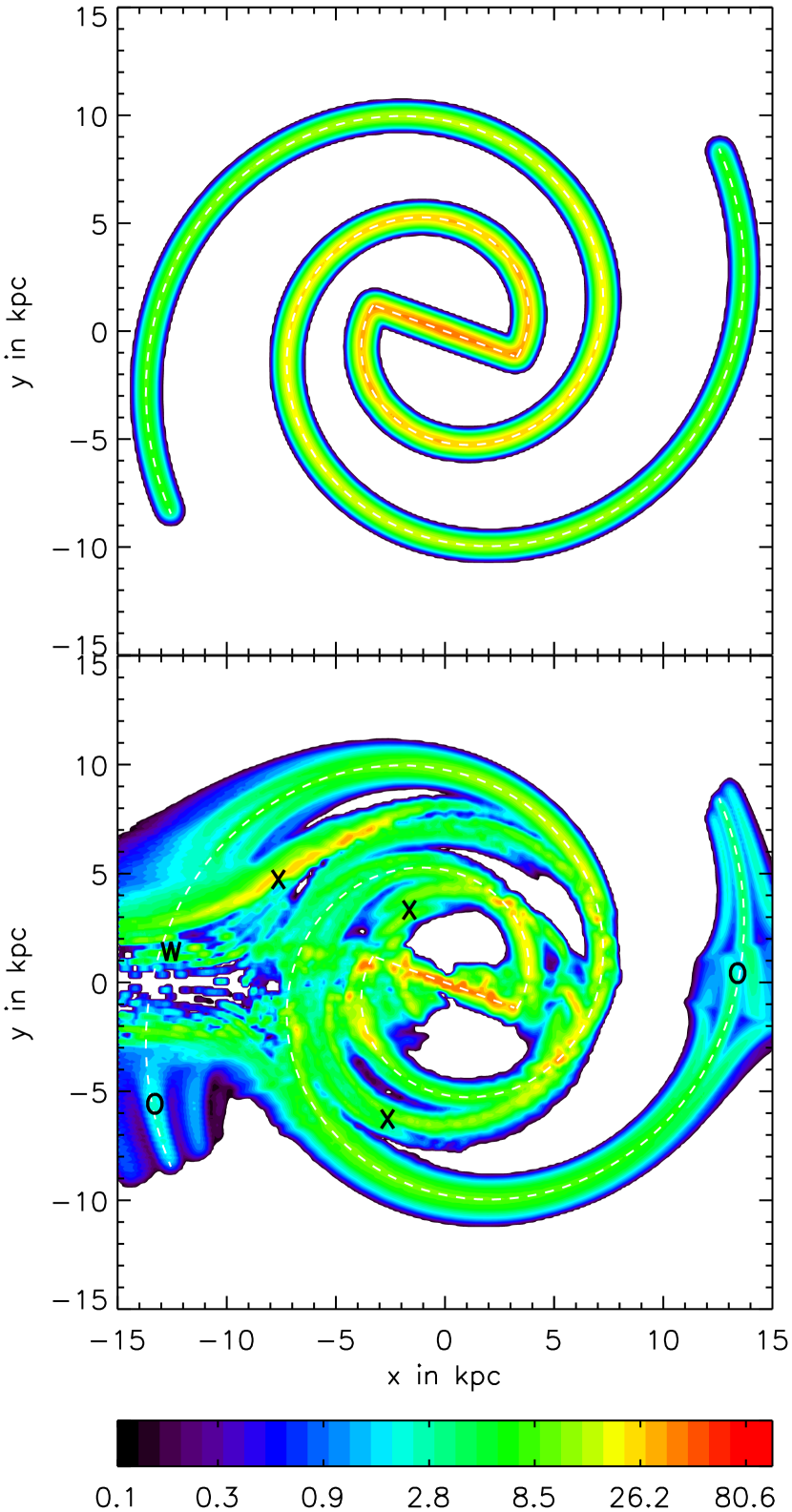
The bottom panel of figure 4 shows the reconstructed surface mass density. To be noted from the figure are three major types of artefacts that we will see again in the deconvolutions of the real data set. In the regions indicated by the letter O, in the anticenter and outside the solar circle on the far side of the Galaxy, the kinematic resolution is poor or nonexistent, and the deconvolution tends to break up the arms into three quasi-parallel structures. The region labelled W at large negative $x$ has no kinematic resolution, but receives some signal at zero velocity, which appears here as a tail on the far side of the Galaxy. The signal in the regions marked with the letter X corresponds to the far distance solution of gas in the spiral arm that passes the sun at about 1 kpc distance. A detailed inspection shows that the very high reconstructed surface mass density in the region at $(x,y)=(-8.,5.)$ arises from an unusually wide z-distribution. Signal in the wing of the line profile of the highest possible velocity near the sun has a velocity, for which only a far solution exists. The deconvolution code cannot perfectly separate shift on account of the intrinsic line width from shift arising from the Galactic gas flow, so a fraction of the signal is attributed to the far solution, which is about 20 times as distant as the near solution, and so the misplaced signal corresponds to a substantial surface mass density, even though it is inconspicuous in the distribution in distance of the gas density.

Figure 5: The deconvolved integrated CO line intensity per distance bin of 100 pc for the Galactic Center direction (top panel) and at 20 degrees positive longitude (bottom). Note the difference in scale.

4 Results

4.1 The standard gas-flow model

Figure 5 shows the deconvolved gas distribution (more precisely the integrated line intensity, $W_{\rm CO}$, per distance bin of 100 pc), for two lines-of-sight, based on the standard gas-flow model with bar inclination angle $\phi=20^{\circ}$. The top panel refers to the direction of the Galactic Center and can therefore be directly compared with Figures 1 and 2, which show the velocity-distance relation and the CO line spectrum for that line-of-sight. Even though in the $W_{\rm CO}$ distribution we see a strong narrow peak near the Galactic Center at 8 kpc distance, a similar fraction of the line signal is in fact placed between about 9 and 10 kpc distance. This corresponds to intensity at 50–100 km/s velocity, for which two distance solutions exist with significantly different $|dv/dD|$. The two solutions are equivalent in terms of the other weight factors, so they receive the same intensity in total, which in the case of the larger distance is spread out over about ten distance bins.

Figure 6: The surface mass density of the Galaxy in M_⊙/pc² assuming a constant conversion factor $X=2.3\cdot 10^{20}\ {\rm molecules/cm^{3}/(K\,km\,s^{-1})}$. The dotted white circle outlines the location of artefacts arising from forbidden velocities. The dashed white lines illustrate the location of the Galactic bar and two possible logarithmic spiral arms, that would correspond to the Sagittarius arm and the Norma/Perseus +l arm. The data are smoothed to about 200 pc resolution to better show the large-scale structure. White areas have a surface mass density below the lower limit of the colorbar.

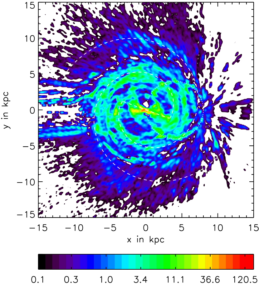
Figure 6 shows the reconstructed surface mass density of molecular gas for the standard gas-flow model and a constant conversion factor $X=2.3\cdot 10^{20}\ {\rm molecules/cm^{3}/(K\,km\,s^{-1})}$ smoothed to about 200 pc resolution. The location of the sun is $x=8\,{\rm kpc}$ and $y=0$. The artefact labelled W in figure 4 is prominent here as well: The patches of relatively high surface mass density at large Galactocentric radii on the far side of the Galaxy (at $x\lesssim-10$ kpc) originate from line signal near zero velocity, for which those large distances are a valid kinematic solution. In some cases the line intensity at small velocities is so high, that signal corresponding to a few M_⊙/pc² survives the filtering with the Gaussian prior that we use to reduce the weights for these solutions.

Also visible in figure 6 are artefacts arising from gas at forbidden velocities in the inner Galaxy. Gas at forbidden velocities is placed where the corresponding extremum in the line-of-sight velocity is found. For circular rotation with constant speed the location of that extremum would delineate a circle of radius $R_{0}/2$ that extends from the sun to the Galactic Center and is indicated by the dotted white line. One can clearly see patches of high surface mass density that roughly follow the dotted line. While it should be expected that the gas resides near the location of the peak in the line-of-sight velocity, the spatial concentration of the gas is most likely exaggerated. The fact that a substantial fraction of the total CO line signal is placed near the dotted white line indicates that the gas flow model underestimates the flow velocities in the inner Galaxy. Note, that this kind of artefact is not seen in test simulation presented in the previous section.

One clearly sees a mass concentration along the Galactic bar where the surface mass density is often two orders of magnitude higher than at similar Galactocentric radii on the sides of the bar. Two spiral arms seem to emerge at the ends of the bar. The distribution of molecular gas supports the notion that those two spiral arms have a small pitch angle. The dashed white line indicates the location of the Galactic bar according to Bissantz et al. (2003) and, for illustration, two logarithmic spiral arms with pitch angle $11.5^{\circ}$, that emanate from the ends of the bar at $R=3.5$ kpc. On the near side this would be the Norma arm that circles around the Galactic Center and reappears as the Perseus +l arm in the notation of Vallée (2002). Emerging on the far side and closely passing by the sun would be the Sagittarius arm. To be noted from the figure is that the distribution of molecular mass is roughly consistent with those two arms. There is excess molecular material that one may associate with two other arms, for example the gas near $x=5$ kpc and $Y=0$ kpc would mark the Scutum arm. The gas between the sun and the outer Perseus +l arm would lie in the Perseus arm. While certain structures in the map can be associated with those arms as discussed in the literature, it is not a priori clear that those structures are real. A comparison with the deconvolved mass distribution for the simulated data set in Fig. 4 shows that the excess material coincides with two artefacts marked by an X at $(x,y)=(-2,3)$ kpc and at $(x,y)=(-2,-7)$ kpc, that correspond to the far solution of the nearby Norma arm and Sagittarius arm, respectively. On the other hand, the gas distribution in the SPH simulation of Bissantz et al. (2003) does not simply follow the logarithmic spiral arms, in particular not within the inner few kpc. While the signal at $(x,y)=(-2,-7)$ kpc is close to the boundary of the SPH simulation region, thus hindering a fair assessment of their relevance, the structure near $(x,y)=(-2,3)$ kpc has a clear counterpart in the gas distribution according to the gas model of Bissantz et al. (2003).

Figure 7: The surface mass distribution in the inner 10 kpc $\times$ 10 kpc of the Galaxy in full resolution. As before the units are M_⊙/pc² assuming a constant conversion factor $X=2.3\cdot 10^{20}\ {\rm molecules/cm^{3}/(K\,km\,s^{-1})}$. White areas have a surface mass density below the lower limit of the colorbar.

Figure 8: Blow-up of the inner 2 kpc $\times$ 2 kpc of Figure 7. The diamond marks the position of the Galactic Center. The solid circle outline the massive cold torus structured inferred by Launhardt et al. (2002). The dotted lines indicate the central molecular zone according to the model of Ferrière et al. (2007). The inner ellipse corresponds to the peak in surface mass density, and the outer ellipse outline the perimeter where the density has fallen to $1/e$ of the peak value. White areas have a surface mass density below the lower limit of the colorbar.

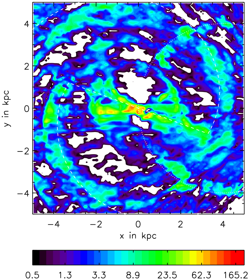
Figure 7 shows the surface-mass distribution within 5 kpc from the Galactic Center with standard resolution of 100 pc. As before the dashed lines indicate the bar and two logarithmic spiral arms, whereas the dotted lines outlines the circle on which gas at forbidden velocity may be projected. Many of the structures shown in Figs. 6 and 7 do not appear as clean and narrow as those in the SPH simulations of Bissantz et al. (2003), but the fact that the most salient features can be recovered lends credibility to their existence in the Galaxy. Particularly interesting are the pseudo-arms that emerge from the bar at about 2 kpc from the Galactic Center. Our deconvolution shows similar structures at $(x,y)=(2,0)$ kpc and $(x,y)=(2,0)$ kpc, although a significant fraction of the latter is clearly gas at the Galactic Center that is misplaced at the far solution (compare Fig. 1).

Within 1 kpc from the Galactic Center the model velocities are affected by the limited resolution of the SPH simulation. One may therefore not expect the gas distribution to be well reproduced. Figure 8 shows the reconstructed distribution of molecular gas within 1 kpc of the Galactic Center. To be noted from the figure is the concentration of molecular gas in three segments that may be interpreted as fragments of an elongated ring that is somewhat off-center, shifted toward positive longitudes (negative $y$). The overall geometry resembles the expanding molecular ring proposed much earlier by Scoville (1972), but stretched along the line-of-sight. Fig. 8 should be interpreted very carefully, because the limited resolution of the gas flow model has a significant impact on the reconstructed gas distribution. In fact we find that it depends on how one interpolates the gas velocity between the grid points at which the average flow velocity is computed in the SPH simulation. For comparison we indicate the location of the massive cold torus found by Launhardt et al. (2002) using IRAS and COBE/CIRBE data by the solid white line. We can further compare our results with those of Sawada et al. (2004) who used only observational data (emission vs. absorption) and no kinematic tracing. They find an center-filled ellipsoidal configuration with large inclination angle to the line-of-sight. The peak in surface density appears at $x\approx-0.03$ kpc and $y\approx-0.15$ kpc (our coordinate system) and may be identified with Sgr B and what they denote the 1.3^∘ region. In contrast, we find the peak in mass density clearly behind the Galactic Center at $x\approx-0.3$ kpc, and the gas distribution is closer to a ring or two arms as suggested by Sofue (1995). Ferrière et al. (2007) have proposed a model of the central molecular zone that appears to be a compromise between the various configurations discussed in the literature. The overall appearance of the central molecular zone is that of an ellipse with a slight reduction of the density toward the center, which is indicated in figure 8 by dotted lines. The inner ellipse corresponds to the peak in surface mass density, and the outer ellipse outline the perimeter where the density has fallen to $1/e$ of the peak value. The major axis of the ellipse is nearly perpendicular to the line-of-sight, whereas in our model it is significantly stretched along the line-of-sight, probably as a result of the limited resolution of the gas flow model. We find no counterpart to the kpc-scale Galactic Bulge disk in the model of Ferrière et al. (2007), in fact our reconstructed surface mass densities to the sides of the bar are very much lower than in her model, if one accounts for a small X-factor in the Galactic Center region. Both in the SPH simulation of Bissantz et al. (2003) and in our surface density maps one sees a concentration of gas along the bar and large voids to the side, which are intersected by pseudo-arms.

4.2 Alternative gas-flow models

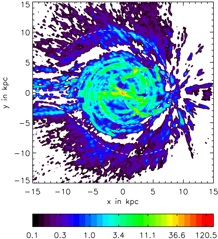
The gas-flow models are not perfect, for example they may not match both the observed terminal-velocity curve (TVC) in the inner Galaxy and the orbit velocity at the solar radius to better than 5%. To investigate the impact of the particular choice of the gas-flow model on the reconstructed gas distribution, we here show deconvolutions based on two alternative models. The first is also derived from a SPH simulation of Bissantz et al. (2003), but in this case the bar is assumed to be inclined at $\phi=30^{\circ}$. This model should reproduce the terminal velocity curve in the longitude range $10^{\circ}\leq l\leq 60^{\circ}$, and thus be qualitatively similar to the standard model, except the bar parameters are different and the overall fit of the model to the lv-diagram is slightly worse but still in agreement with observations. Figure 9 shows the reconstructed surface mass density for this alternative gas-flow model. To be noted from the figure are the large voids at Galactocentric radii $R=(7-8)$ kpc, whereas the mass density in the inner 6 kpc is more homogeneous than for the standard model. Figure 9 clearly shows an increased amount of material in artefacts along the dotted circle, which indicates that the standard model is more in agreement with the observed gas flow, as expected.

Figure 9: The surface mass density in M_⊙/pc² for the alternative gas-flow model with bar inclination $\phi=30^{\circ}$. The dashed line indicating the location of the bar and two logarithmic spiral arms is plotted accordingly. White areas have a surface mass density below the lower limit of the colorbar.

Whereas the first alternative gas-flow model should still be a fair approximation of the actual velocity distribution in the inner Galaxy, we now also use a model that is intentionally distorted to no longer reproduce the TVC in the inner Galaxy. For that purpose we rotate the standard gas-flow model by another $20^{\circ}$, so that the bar inclination is $\phi=40^{\circ}$. As shown in Fig. 10, the resultant gas distribution is significantly changed. There is a large void between the sun and the Galactic Center at about $(x,y)=(5,-1)$ kpc, where the line-of-sight velocity in the flow model no longer matches any signal in the CO line. A second large void appear in the lower left of the plot, corresponding to a Galactic longitude $l\approx 30^{\circ}$ and distances around 15 kpc. A relatively high surface mass density is found on the far side of the Galaxy at 7 kpc Galactocentric radius which is most likely misplaced line signal from the Galactic Center region.

Figure 10: The surface mass density in M_⊙/pc² for the standard gas-flow model rotated by another $20^{\circ}$, so that the bar inclination is $\phi=40^{\circ}$. This gas-flow that is intentionally distorted to no longer reproduce the actual velocity distribution in the inner Galaxy.

5 Summary

We have derived a new model of the distribution of molecular gas in the Galaxy based on CO line emission (Dame et al., 2001). For that purpose we use a gas-flow model derived from smoothed particle hydrodynamics (SPH) simulations in gravitational potentials based on the NIR luminosity distribution of the bulge and disk (Bissantz et al., 2003). Besides providing a more accurate picture of cloud orbits in the inner Galaxy, a fundamental advantage of this model is that it provides kinematic resolution toward the Galactic Center, in contrast to standard deconvolution techniques based on purely circular rotation.

To test the deconvolution procedure and estimate the nature and strength of deconvolution artefacts, we have applied it to a simulated CO line data set based on a model gas distribution that consists of a bar and two spiral arms. We have also deconvolved the actual observed CO data using alternative gas-flow models, one of which is intentionally distorted to no longer reproduce the actual velocity distribution in the inner Galaxy. The reconstructed distribution of surface mass density is significantly affected in the case of the ill-fitting gas-flow model. When using gas-flow models that reproduce the terminal-velocity curve, but are based on different bar inclination angles, the reconstructed gas distribution are much more alike. In particular, the deconvolution is robust against a simple rescaling of the gas-flow velocities by a few percent. A comparison of the surface mass density determined using feasible and unfeasible gas flow models shows that in the latter case the resulting surface mass density is also unfeasible. Examples of that are the very low surface mass density regions around $(x,y)=(5,-1)\,$kpc and $(x,y)=(-8,-8)\,$kpc, and the strong feature at $(x,y)=(-7,-1)\,$kpc in Figure 10. Hence, the comparison of the surface mass densities from the various gas flow models strongly indicates that the result of the deconvolution algorithm is robust against moderate variations in the underlying gas flow model. On the other hand, it is sensitive enough to changes in the gas flow model to discriminate the surface mass density solutions based on feasible gas-flow models against those based on unfeasible flow models.

We now describe our model for the surface mass density of the gas in more detail. In the model we find a concentration of mass along the Galactic bar where the surface mass density is often two orders of magnitude higher than at similar Galactocentric radii of the sides of the bar. Two spiral arms seem to emerge at the ends of the bar, which have a small pitch angle $\sim 12^{\circ}$. While certain structures in the surface density distribution may be associated with two more spiral arms as discussed in the literature (Vallée, 2002), the evidence for those arms provided by this deconvolution is not strong, and localizing spiral arms based on kinematics and CO line data alone is difficult. We also reproduce a concentration of molecular gas in the shape of an elongated ring around the Galactic Center that resembles the massive cold torus found by Launhardt et al. (2002), but is broken up and somewhat stretched along the line-of-sight, probably as a result of the limited resolution of the gas flow model.

Models of the three-dimensional distribution of molecular gas in the Milky Way Galaxy can be used in many applications, for example to analyze the diffuse Galactic gamma-ray emission that will be observed with GLAST. Knowledge of the gas distribution is essential for studies of the cosmic-ray gradient in the Galaxy, but also for investigation of small-scale variations in the density and flux of cosmic rays. Our gas model will be publicly available at http://cherenkov.physics.iastate.edu/gas.

References

- Arimoto et al. (1996) Arimoto, N., Sofue, Y., Tsujimoto, T., 1996, PASJ, 48, 275
- Babusiaux & Gilmore (2005) Babusiaux, C., and Gilmore, G., 2005, MNRAS, 358, 1309
- Benjamin et al. (2005) Benjamin, R.A., et al., 2005, ApJ, 630, L149
- Bertsch et al. (1993) Bertsch, D.L., et al., 1993, ApJ, 416, 587
- Binney & Merrifield (1998) Binney, J., Merrifield, M., 1998, Galactic Astronomy, Princeton University Press, Princeton, New Jersey
- Bissantz et al. (1997) Bissantz, N., Englmaier, P., Binney, J., Gerhard O., 1997, MNRAS, 289, 651
- Bissantz et al. (2003) Bissantz, N., Englmaier, P., and Gerhard, O., 2003, MNRAS, 340, 949
- Bissantz & Gerhard (2002) Bissantz, N., Gerhard, O., 2002, MNRAS, 330, 591
- Burgh et al. (2007) Burgh, E.B., France, K., McCandliss, S.R., 2007, ApJ, 658, 446
- Clemens et al. (1986) Clemens, D.P., Sanders, D.B., Scoville, N.Z., Solomon, P.M., 1986, ApJS 60, 297
- Dahmen et al. (1998) Dahmen, G., Hüttemeister, S., Wilson, T.L., Mauersberger, R., A&A, 331, 959
- Dame et al. (2001) Dame, T.M., Hartmann, D., and Thaddeus, P., 2001, ApJ, 547, 792
- Dehnen & Binney (1998) Dehnen, W., Binney, J.J., 1998, MNRAS, 298, 387
- Dickman (1978) Dickman, R.L., 1978, ApJS, 37, 407
- Englmaier & Gerhard (1999) Englmaier, P., Gerhard, O., 1999, MNRAS, 304, 512
- Ferrière et al. (2007) Ferrière, K., Gillard, W., and Jean, P., 2007, A&A, 467, 611
- Gerhard (2001) Gerhard, O., 2001, in Galaxy disks and disk galaxies, ASP Conf. Ser. Vol. 230, eds. Funes & Corsini, p.21
- Heyer et al. (1998) Heyer, M.H., et al., 1998, ApJS, 115, 241
- Hunter et al. (1997) Hunter, S.D., et al., 1997, ApJ, 481, 205
- Joshi (2007) Joshi, Y.C., 2007, MNRAS, 378, 768
- Launhardt et al. (2002) Launhardt, R., Zylka, R., Mezger, P.G., 2002, A&A, 384, 112
- Levine et al. (2006) Levine, E.S., Blitz, L., Heiles, C., 2006, ApJ, 643, 881
- Malhotra (1994) Malhotra, S., 1994, ApJ, 433, 687
- McClure-Griffiths & Dickey (2007) McClure-Griffiths, N.M., Dickey, J.M., 2007, ApJ, 671, 427
- Nakagawa et al. (2007) Nakagawa, M., Onishi, T., Mizuno, A., Fukui, Y., 2005, PASJ, 57, 917
- Nakanishi & Sofue (2006) Nakanishi, H., Sofue, Y., 2006, PASJ, 58, 847
- Oka et al. (1998) Oka, T., et al., 1998, ApJ, 498, 730
- Olling & Merrifield (1998) Olling, R.P., Merrifield, M.R., 1998, MNRAS, 297, 943
- Oort et al. (1958) Oort, J.H., Kerr, F.T., Westerhound, G., 1958, MNRAS, 118, 379
- Pohl & Esposito (1998) Pohl, M., Esposito, J.A., 1998, ApJ, 507, 327
- Sawada et al. (2004) Sawada, T., Hasegawa, T., Handa, T., Cohen, R.J., 2004, MNRAS, 349, 1167
- Scoville (1972) Scoville, N.Z., 1972, ApJ, 175, L127
- Sodroski et al. (1995) Sodroski, T.J., Odegard, N., Dwek, E., et al., 1995, ApJ, 452, 262
- Sofue (1995) Sofue, Y., 1995, PASJ, 47, 527
- Sreekumar et al. (1998) Sreekumar, P., et al., 1998, ApJ, 494, 523
- Strong et al. (2004) Strong, A.W., Moskalenko, I.V., Reimer, O., et al., 2004, A&A, 422, L47
- Vallée (2002) Vallée, J.P., 2002, ApJ, 566, 261
- Wall (2006) Wall, W.F., 2006, RMAA, 42, 117, (see also astro-ph/0610209)
- Wouterloot et al. (1990) Wouterloot, J.G.A., Brand, J., Burton, W.B., Kwee, K.K., 1990, A&A, 230, 21