Lab/UFR-HEP0701/GNPHE/0701
Non Planar Topological 3-Vertex Formalism

Abstract

Using embedding of complex curves in the complex projective plane $\mathbb{P}^{2}$, we develop a non planar topological 3-vertex formalism for topological strings on the family of local Calabi-Yau threefolds $X^{\left(m,-m,0\right)}=\mathcal{O}(m)\oplus\mathcal{O}(-m)\rightarrow E^{\left(t,\infty\right)}$. The base $E^{\left(t,\infty\right)}$ stands for the degenerate elliptic curve with Kahler parameter $t$; but a large complex structure $\mu$; i.e $\left|\mu\right|\longrightarrow\infty$. We also give first results regarding A-model topological string amplitudes on $X^{\left(m,-m,0\right)}$. The $2D$ $U\left(1\right)$ gauged $\mathcal{N}=2$ supersymmetric sigma models of the degenerate elliptic curve $E^{\left(t,\infty\right)}$ as well as for the family $X^{\left(m,-m,0\right)}$ are studied and the role of D- and F-terms is explicitly exhibited.
Key words: Topological String, Topological Vertex, Hypersurfaces in the Local Projective Plane. Supersymmetric Linear Sigma Models with D- and F-terms.

1 Introduction

Topological string theory [1, 2, 3] is a powerful method to deal with the $4D$ $\mathcal{N}=2$ supergravity Planck limit of the compactification of type II superstring on Calabi-Yau (CY) threefolds X₃ [4, 5]. The study of local Gromov-Witten theory of curves in non compact Calabi-Yau threefolds [6, 7, 8, 9, 10] and the OSV conjecture [11], relating microscopic 4D black holes to 2D q-deformed Yang-Mills theory [12]-[18], have given an additional impulse to the revival interest in the study of the topological field and string theories [19]-[26]. Several important results have been obtained in the few last years; in particular the development of the topological tri-vertex ( to which we refer below as planar 3-vertex) method for computing the A-model partition function for non compact toric CY3s [28, 29] and the interpretation of this vertex in terms of 3d-partitions of melting crystals generalizing $U\left(\infty\right)$ Young tableau  [30, 31].

Moreover the planar 3-vertex and its refined version [32, 33] have been shown particularly powerful. They agree with the Nekrasov’s partition function of $\mathcal{N}=2$ $SU(N)$ gauge theory [34]-[40] and provide more insights into non perturbative dynamics of string field theory. The power of the topological 3-vertex method may be compared with the power of Feynman graphs technique in perturbative $\phi^{3}$ quantum field theory (QFT). This formal similarity between the toric web-diagrams and the Feynman graphs opens a window on the following issues:
First, the use of perturbative QFT results to motivate topological stringy analogues, in particular toric web-diagrams with higher dimensional vertices such as the typical $\phi^{4}$ to be considered in this study;
Second, the development of new techniques to enlarge the class of toric Calabi-Yau threefolds to which the topological vertex formalism applies.

Recall that for non compact toric Calabi-Yau threefolds $X_{3}$ with toric web-diagram $\Delta\left(X_{3}\right)$, the planar 3-vertex method allows to compute explicitly the A- model topological string amplitudes. The topological vertex method is a Feynman-rules like technique where the Feynman graphs, the vertices of these graphs, the momenta, and the propagators correspond respectively to the toric web-diagrams $\Delta\left(X_{3}\right)$, the 3-valent vertices $C_{\lambda\mu\nu}$, Young diagrams $\lambda$, and the weights $\left(-\right)^{\left(n+1\right)\left|\lambda\right|}e^{-t\left|\lambda\right|}q^{-\frac{n}{2}\kappa\left(\lambda\right)}$ where $n$ encodes the framing.

Motivated by:
(1) the formal correspondence between toric web-diagrams of local Calabi-Yau threefolds and QFT Feynman graphs,
(2) the two classes of toric Calabi-Yau threefolds describing the vacua of supersymmetric sigma model with (W$\left(\Phi_{i}\right)\neq 0$) and without superpotential (W$\left(\Phi_{i}\right)=0$) , and
(3) a special feature of the local 2- torus $\mathcal{O}(m)\oplus\mathcal{O}(-m)\rightarrow E^{\left(t,\infty\right)}$ where the elliptic curve

$$E^{\left(t,\mu\right)}$$ (1.1)

is in the base of the local Calabi-Yau threefold $X^{\left(m,-m,0\right)}$ rather than in the fiber,
we address in this paper, the two following points:
(a) We propose in this study a toric representation for the family of the local 2-torii with fixed finite Kahler parameter $t$ and a large complex structure $\mu$; say $\left|\mu\right|\longrightarrow\infty$,

$$\mathcal{O}(m)\oplus\mathcal{O}(-m)\rightarrow E^{\left(t,\infty\right)},$$ (1.2)

with integer $m$. The degenerate elliptic curve

$$E^{\left(t,\infty\right)},$$ (1.3)

describing the base of the above local Calabi-Yau threefolds (1.2), will be realized as the (toric) boundary of the complex toric projective plane $\mathbb{P}^{2}$; see sections 3, 5 and 6 as well as the appendix for more details.
With this representation at hand, we can then:
($\mathbf{\alpha}$) circumvent, at least for the particular case of the degenerate $E^{\left(t,\infty\right)}$, the usual difficulty regarding the lack of a toric diagram for the 2-torus.
In addition to the large complex structure limit constraint $\left|\mu\right|\rightarrow\infty$, the other price to pay in this set up is to consider a non planar 3-vertex formalism rather than the standard planar 3-vertex one based on the $R\times T^{2}$ special Lagrangian fibration of $\mathbb{C}^{3}$. The reason behind the emergence of the non planar 3-vertex is that the toric Calabi-Yau 3-fold $X^{\left(m,-m,0\right)}$ is realized as a non compact toric hypersurface of the complex four dimensional toric manifold

$$\mathcal{O}(m)\oplus\mathcal{O}(-m)\rightarrow\mathbb{P}^{2}.$$ (1.4)

For later use, we will refer to the local geometries (1.2) and (1.4) as $H_{3}$ and $Y_{4}$ respectively.
The geometry $Y_{4}$ will be also promoted to the Calab-Yau 4-fold $X_{4}=\mathcal{O}(-m-3)\rightarrow W\mathbb{P}_{1,1,1,m}^{3}$.
($\mathbf{\beta}$) draw the lines for computing the topological amplitudes by using a non planar 3-vertex formalism.
In the present study, we will mainly set up the key idea by:
(i) building the toric web-diagram $\Delta\left(X_{3}\right)$ of the local degenerate elliptic curve $X^{\left(m,-m,0\right)}$.
(ii) give first results regarding the structure of the topological non planar 3-vertex and the partition function of $X^{\left(m,-m,0\right)}$ as well as their relation to the 4- vertex of the ambient $\mathbb{C}^{4}$ local patch and to the generalized Young diagrams.
(b) We develop the supersymmetric linear sigma model field theory setting of the local degenerate elliptic curve $X^{\left(m,-m,0\right)}$.
More precisely, we show the two main following things:
($\mathbf{\alpha}$) the planar 3-vertex method is associated with the auxiliary D-terms in supersymmetric sigma models.
The non planar 3-vertex formalism we will be considering here corresponds to the case where we have both D-terms and F-terms.
($\mathbf{\beta}$) We use the sigma model for local $\mathbb{P}^{2}$ to induce the $\mathcal{N}=2$ supersymmetric gauged model for the local elliptic curve $X^{\left(m,-m,0\right)}$. The underlying complex geometry of a such construction was noticed in the Witten’s original work [47]. Here, we give explicit details regarding the implementation of F-terms.

The organization of this paper is as follows: In section 2, we give an overview of the topological planar 3- vertex method. In section 3, we exhibit briefly first results concerning the topological non planar 3-vertex by considering the example of a Calabi-Yau threefold $H_{3}$. The toric 3-fold $H_{3}$ is realized as a hypersurface of a four dimensional complex Kahler manifold. In section 4, we review the main points of the $U\left(1\right)$ gauged supersymmetric sigma model realization of the local $\mathbb{P}^{2}$. In section 5, we consider the sigma model for the degenerate local elliptic curve $X^{\left(m,-m,0\right)}$. As the question of the toric realization of $\mathbb{T}^{2}$ is a crucial point, we divide this section in three parts: We first study the realization of the degenerate elliptic curve $E^{\left(t,\infty\right)}$ by using the compact divisor of $\mathbb{P}^{2}$. Then we give explicit details regarding the $U\left(1\right)$ gauged supersymmetric sigma model realization of the local degenerate elliptic curve $X^{\left(m,-m,0\right)}$. Next, we study the moduli space of the supersymmetric vacua associated with $X^{\left(3,-3,0\right)}$. In section 6, we extend the construction to the case of local elliptic curve $X^{\left(m,-m,0\right)}$. In section 7, we give the conclusion and in section 8 we give an appendix where we show that $\partial\left(\mathbb{P}^{2}\right)$ is precisely $E^{\left(t,\infty\right)}$.

2 Topological vertex method

In this section, we consider the topological 3-vertex method used for the computation of the A- model topological string amplitudes. We illustrate this method through some examples of non compact toric Calabi-Yau threefolds namely:
(1) the complex space $\mathbb{C}^{3}$, with special Lagrangian fibration as $R\times T^{2}$, playing the role of the planar 3-vertex.
(2) the resolved conifold obtained by gluing two planar 3-vertices,
(3) local $\mathbb{P}^{2}$ made of three planar 3-vertices.
Then, we consider an example of toric Calabi-Yau threefold (1.2) where one needs introducing non planar 3-vertices (and 4-vertices). This local Calabi-Yau threefold is precisely the one given by the local degenerate elliptic curve $X^{\left(m,-m,0\right)}=\mathcal{O}(m)\oplus\mathcal{O}(-m)\rightarrow E^{\left(t,\infty\right)}$ realized as a hypersurface in (1.4).

2.1 Tri-vertex method: A brief review

The topological 3-vertex formalism computes the partition function

$$Z_{X_{3}}(q)$$

of the local toric Calabi-Yau threefolds $X_{3}$. In this formalism, the toric web-diagram of $X_{3}$ is thought of as resulting from gluing copies of planar 3-vertices $C_{\lambda\mu\nu}$ along their edges.
Recall that the topological vertex $C_{\lambda\mu\nu}$ has three legs ending on stacks of Lagrangian D-branes ($\mathbb{C}\times S^{1}$) represented by 2d partitions $\lambda$, $\mu$ and $\nu$.
The partition function $Z_{X_{3}}(q)$ depends on the following quantities:
(i) the parameter $q$ which reads in terms of the string coupling as $e^{-g_{s}}$; it plays the role of the Boltzmann weight.
(ii) the Kahler parameters $\left\{t_{i}\right\}$ of the local Calabi-Yau threefold $X_{3}$ ( $i=1,...,h^{1,1}\left(X_{3}\right)$).
Below, we will consider simple examples where

$$h^{1,1}\left(X_{3}\right)=1.$$

(iii) the boundary conditions (open strings) described by $2d$ partitions $\mu$ ( generic representations of $U\left(\infty\right)$). In the QFT language where Feynman graphs play a quite similar role as the toric web-diagrams, the 2d partition $\mu$ corresponds to the ”external momentum” of Feynman graph. Recall that a 2d partition $\mu$ is a Young diagram with columns

$$\left(\mu_{1},\mu_{2},...\right),\qquad\mu_{i}\geq\mu_{i+1},\qquad\mu_{i}\in\mathbb{Z}_{+}.$$ (2.1)

Columns of the 2d partition are associated with Lagrangian D- branes and rows with Lagrangian anti- D-branes.
(iv) Lagrangian D-brane/anti-D-brane pairs are needed for the gluing of the vertices. The gluing operation is achieved by inserting 2d partitions $\nu$ and their transpose $\nu^{T}$ at the cuts and summing over all possible $\nu$’s. In QFT language, $\nu$ corresponds to ”internal momenta”.
The topological 3-vertex method for computing the partition function $Z_{X_{3}}(q)$ is illustrated on the three examples given below.

2.2 Examples

Example 1: the 3-vertex of $\mathbb{C}^{3}$
The toric graph of $\mathbb{C}^{3}$ is given by figure 1.

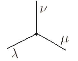
Figure 1: The toric web-diagram of $C^{3}$. It appears as local patches in toric Calabi-Yau threefolds. The three edges end on stacks of Lagrangian D branes. $\lambda,$ $\mu$ and $\nu$ are 2d partitions which, in QFT set up, may be thought of as the external momenta.

Following [28], the partition function of the 3-vertex, with a stack of Lagrangian D-branes ending on its legs captured by the boundary conditions $\left(\lambda,\mu,\nu\right)$, is given by

$$Z_{X_{3}}(q)=\sum_{\lambda,\mu,\nu}C_{\lambda\mu\nu}(q)\left(Tr_{\lambda}\mathcal{V}\text{ }Tr_{\mu}\mathcal{V}\text{ }Tr_{\nu}\mathcal{V}\right).$$ (2.2)

In this relation, the trace $Tr_{\lambda}$ of the holonomy matrix $\mathcal{V}$ , with eigenvalues $x=\left(x_{1},x_{2},...\right)$, is given by the Schur function $\mathcal{S}_{\lambda}(x)$. The latter depends on the 2d partition $\lambda=\left(\lambda_{1},\lambda_{2},...\right)$ and the $x_{i}=q^{i-1/2-\lambda_{i}}$. The rank three tensor

$$C^{\left(3\right)}=C_{\lambda\mu\nu},$$ (2.3)

is the topological 3-vertex whose explicit expression reads as

$$C_{\lambda\mu\nu}(q)=q^{\kappa(\lambda)}\left[\mathcal{S}_{\nu^{T}}(q^{-\rho})\sum_{2d\text{ partitions }\eta}\mathcal{S}_{\lambda^{T}/\eta}(q^{-\nu-\rho})\mathcal{S}_{\mu/\eta}(q^{-\nu^{T}-\rho})\right]$$ (2.4)

with $\rho=\left(\rho_{1},\rho_{2},...\right)$ and $\rho_{i}=1/2-i$.
Eq(2.4) involves the product of skew-Schur functions $\mathcal{S}_{\mu/\eta}$. It reduces, for the closed topological string case, to

$$Z_{\mathbb{C}^{3}}(q)=C_{\emptyset\emptyset\emptyset}(q)=\prod\limits_{n=1}^{\infty}(1-q^{n})^{-n}.$$ (2.5)

which is nothing but the 3d MacMahon function.

Example 2:   Resolved conifold $\ X_{3}=\mathcal{O}\left(-1\right)\oplus\mathcal{O}\left(-1\right)\rightarrow\mathbb{P}^{1}$
The resolved conifold has one Kahler parameter $t$ parameterizing the size of the projective line $\mathbb{P}^{1}$. Figure 2 describes its toric web-diagram.

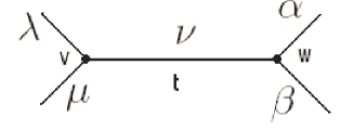
Figure 2: Resolved conifold $\mathcal{O}\left(-1\right)\oplus\mathcal{O}\left(-1\right)\rightarrow P^{1}$ made of two planar 3-vertices.

This local threefold $X_{3}$ is obtained by gluing two 3-vertices along one edge leaving then four opened external legs.
In the simplest case where there is no boundary terms on the external legs, the partition function of the closed topological string on the resolved conifold is given by,

$$Z_{X_{3}}(q,t)=\sum_{\text{2d partitions }\nu}C_{\emptyset\emptyset\nu}(q)\text{ }(-1)^{\left|\nu\right|}e^{-\left|\nu\right|t}\text{ }C_{\emptyset\emptyset\nu^{T}}(q)\text{.}$$ (2.6)

In this relation, $\nu^{\mathrm{T}}$ is the transpose of the 2d partition $\nu$ with $\left|\nu\right|$ boxes and $C_{\emptyset\emptyset\nu}(q)$ is as in eq(2.4) by setting the boundary conditions as $\lambda=\emptyset$ and $\mu=\emptyset$.

Example 3:   Local $\mathbb{P}^{2}:$ $\ X_{3}=\mathcal{O}\left(-3\right)$ $\ \mathbb{\rightarrow P}^{2}$
The local $\mathbb{P}^{2}$ has one Kahler modulus $t$ parameterizing the size of the projective plane $\mathbb{P}^{2}$. Figure 3 describes its toric web-diagram.

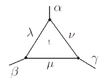
Figure 3: Toric web-diagram of $\mathcal{O}\left(-3\right)\rightarrow\mathbb{P}^{2}$ made of three planar vertices

This local threefold is obtained by gluing three 3-vertices. For simplicity, we consider here also the case where there is no boundaries. The corresponding partition function reads as follows:

$$Z_{X_{3}}(q,t)=\sum_{\lambda,\mu,\nu}C_{\emptyset\mu\nu^{T}}(q)C_{\lambda\mu^{T}\emptyset}(q)\text{ }C_{\lambda^{T}\emptyset\nu}(q)(-e^{-t})^{\left|\nu\right|+\left|\lambda\right|+\left|\nu\right|}q^{\kappa(\lambda)+\kappa\left(\mu\right)+\kappa(\nu)}$$ (2.7)

with

$$\kappa(\lambda)=2\left[\left(\left\|\lambda\right\|^{2}-\left|\lambda\right|\right)-\left(\left\|\lambda^{T}\right\|^{2}-\left|\lambda^{T}\right|\right)\right],$$ (2.8)

being the Casimir of the 2d partition.

3 Beyond the planar vertex method

First, we describe briefly the field theory setting of the local elliptic curve geometry leaving technical details for next sections. Then we give our first results regarding the topological non planar 3-vertex formalism and the explicit expression of the partition function associated with eq(1.2).

3.1 Field theory set up

The local CY3 examples we have described above have toric web-diagrams involving planar 3- vertices; see figures (1)-(2)-(3). These toric threefolds $X_{3}$ have a very remarkable field theory set up; they describe supersymmetric vacua of 2D $\mathcal{N}=2$ linear sigma model with $U^{r}\left(1\right)$ gauge symmetry and $\left(r+3\right)$ matter multiplets $\Phi_{i}$,

$$U^{r}\left(1\right):\qquad\Phi_{j}\equiv e^{iq_{j}^{a}}\Phi_{j},\qquad a=1,...,r,$$ (3.1)

The defining eq of $X_{3}$ is given by the field equation of motion of the $D^{a}$ auxiliary fields,

$$X_{3}:\qquad\frac{\delta\mathcal{L}}{\delta D^{a}}=\sum_{i=1}^{r+3}q_{i}^{a}\left|z_{i}\right|^{2}=0,\qquad$$ (3.2)

where the field coordinates $z_{i}$ are the leading components of the chiral superfields $\Phi_{i}$ and where

$$\sum_{i=1}^{r+3}q_{i}^{a}=0,\qquad a=1,...,r,$$ (3.3)

stands for the Calabi-Yau condition.

Toric Calabi-Yau threefolds can be also realized as hypersurfaces $H_{3}$ in higher d- dimension complex Kahler toric manifolds $\mathcal{Y}_{d}$,

$$H_{3}\subset\mathcal{Y}_{d},\qquad d\geq 4.$$ (3.4)

Locally, the Kahler toric d-fold $\mathcal{Y}_{d}$ may be imagined as given by the toric fibration $R^{d}\times T^{d}$ or as $R^{d}\times F_{d}$ with fiber $F_{d}=R\times T^{d-1}$. The toric web-diagram of $\mathcal{Y}_{d}$ involve d- dimensional vertices where shrink all the 1-cycles of the toroidal fibration.

Figure 4: A generic toric web-diagram of a 4-vertex. In toric geometry, this web-diagram corresponds to the real base of the local patch $\mathbb{C}^{4}$.

The toric CY3 hypersurfaces $H_{3}$ have also a supersymmetric field theory setting. It will be developed in details in forthcoming sections, see also the analysis of [47]. The $H_{3}$’s describe as well supersymmetric vacua of 2D $\mathcal{N}=2$ linear sigma model with gauge $\left\{V_{a}\right\}$ and matter $\left\{\Phi_{i}\right\}$ multiplets, $i=1,...,r+d$.
The defining equation of the toric CY hypersurface $H_{3}$ is given by the field equations of motion of both the D- and the F- auxiliary fields,

$$H_{3}:\left\{\begin{array}[]{c}\frac{\delta\mathcal{L}}{\delta D^{a}}=0,\qquad a=1,...,r\\ \frac{\delta\mathcal{L}}{\delta F^{\alpha}}=0,\qquad\alpha=1,...,m\end{array}\right|,$$ (3.5)

with $m=d-3$ and $d\geq 4$. The first $r$ equations, which are similar to eq(3.2), reduce the dimension down to $\left(d-r\right)$. The second equations, which are gauge invariant constraint relations,

$$\left\{\begin{array}[]{c}f_{\alpha}\left(z_{1},...,z_{d}\right)=0\\ f_{\alpha}\left(\mathrm{\lambda}_{1}z_{1},...,\mathrm{\lambda}_{d}z_{d}\right)=0\\ \mathrm{\lambda}_{j}=e^{iq_{j}^{a}\mathrm{\alpha}_{a}}\end{array}\right|,\qquad\alpha=1,...,m,$$ (3.6)

reduce the number of free field variables down to 3; say $\left(w_{1},w_{2},w_{3}\right)$. Up to solving eqs(3.5), one can express all the $z_{i}$ field variables in terms of the $w$’s as shown below

$$z_{i}=z_{i}\left(w_{1},w_{2},w_{3}\right),\qquad i=1,...,r+d.$$ (3.7)

In the next subsection, we study in details the case $d=4$.

3.2 Results on non planar vertex formalism

The results we will give below concern the following:
(1) the toric realization of the local degenerate elliptic curve (1.2),
(2) the set up of the non planar 3- vertex formalism and
(3) the computation of the partition function Z${}_{H_{3}}$.

3.2.1 Local degenerate elliptic curve

Consider the local Calabi-Yau threefold (1.2) and focus on the particular local degenerate elliptic curve,

$$H_{3}=\mathcal{O}(+3)\oplus\mathcal{O}(-3)\rightarrow E^{\left(t,\infty\right)},\qquad m=3.$$ (3.8)

The degenerate elliptic curve $E^{\left(t,\infty\right)}$ is given by the toric boundary (divisor) of the complex projective plane $\mathbb{P}^{2}$,

$$E^{\left(t,\infty\right)}=\partial\left(\mathbb{P}^{2}\right).$$ (3.9)

This is just a compact divisor (hyperline) of $\mathbb{P}^{2}$. The toric web-diagram associated to (3.8) is given by figure 5.

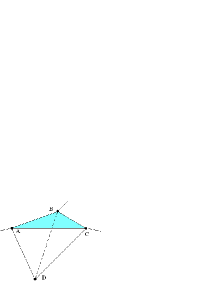
Figure 5: Non planar toric web-diagram of  $\mathcal{O}\left(+3\right)\oplus\mathcal{O}\left(-3\right)\rightarrow E^{\left(t,\infty\right)}$. This is a toric CY3 divisor of the four dimension complex Kahler manifold $\mathcal{O}\left(+3\right)\oplus\mathcal{O}\left(-3\right)\rightarrow P^{2}$  The hollow triangle ABC refers to the degenerate elliptic curve $E^{\left(t,\infty\right)}$. The full triangles ABD, ZCD, BCD refer to the three other projective planes.

The non compact toric 4- fold $\mathcal{Y}_{4}$ of eq(3.4) is given by

$$\mathcal{Y}_{4}=\mathcal{O}(-3)\rightarrow WP_{1,1,1,3}^{3},$$ (3.10)

where $WP_{1,1,1,3}^{3}$ stands for the complex 3- dimension weighted projective space. To keep in touch with the Calabi-Yau condition, we promote $\mathcal{Y}_{4}$ to the toric Calabi-Yau 4-fold

$$X_{4}=\mathcal{O}(-6)\rightarrow WP_{1,1,1,3}^{3},$$ (3.11)

and in general to

$$X_{4}=\mathcal{O}(-3-m)\rightarrow WP_{1,1,1,m}^{3}$$ (3.12)

with $m\geq 1$.

3.2.2 Toric cap and toric cylinder

From eq(3.8), one distinguishes two special divisors of the local degenerate elliptic curve $H_{3}$:
(1) ”toric cap”: see figure 6
This divisor corresponds to $H_{3}$ taken as the fibration $\mathcal{O}(-3)\rightarrow Y_{2}$.  The base $Y_{2}$ is a compact complex surface given by

$$Y_{2}=\mathcal{O}(+3)\rightarrow E^{\left(t,\infty\right)}.$$ (3.13)

The toric web-diagram of the complex surface $Y_{2}$ is exhibited in figure 5:

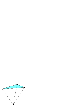
Figure 6: Toric web-diagram of  $\mathcal{O}\left(+3\right)\rightarrow E^{\left(t,\infty\right)}$. This figure looks like a ”toric cap” obtained by gluing three triangles as shown on the figure.

The first Chern class $c_{1}\left(T^{\ast}Y_{2}\right)$ is equal to $+3$. The toric web-diagram of $E^{\left(t,\infty\right)}$ is given by the boundary of the triangle and $\mathcal{O}(+3)$ is a compact line.
The toric web-diagram of $Y_{2}$ is non planar and can be thought of as the triangulation of the topological cap of [28]. Below, we will refer to $Y_{2}$ as the ”toric cap”. Notice also the following features:
(a) the complex surface $Y_{2}$ is a compact divisor of $H_{3}$; it is made of the union of three complex projective planes, which we denote as $\mathbb{P}_{1}^{2}$, $\mathbb{P}_{2}^{2}$ and $\mathbb{P}_{3}^{2}$.
The projective planes $\mathbb{P}_{i}^{2}$ belong to three different $\mathbb{C}^{3}$ spaces of the ambient $\mathbb{C}^{4}$.
(b) the toric web-diagram of $Y_{2}$ is made of three triangles as shown in the figure 6. Recall that the toric web-diagram of a generic projective plane is given by a triangle (figure 3).
The projective planes (triangles) have mutual intersections $I_{ij}$ along complex projective lines (edges) and a non planar tri-intersection vertex $I_{123}$.
(2) toric cylinder
This divisor corresponds to think about $H_{3}$ as the fibration $\mathcal{O}(+3)\rightarrow\widetilde{Y}_{2}$.
Here the base $\widetilde{Y}_{2}$ is a non compact complex surface given by

$$\widetilde{Y}_{2}=\mathcal{O}(-3)\rightarrow E^{\left(t,\infty\right)}.$$ (3.14)

Its first Chern class $c_{1}\left(T^{\ast}\widetilde{Y}_{2}\right)$ is equal to $-3$. Here also the toric web-diagram of $E^{\left(t,\infty\right)}$ is the boundary of the triangle and $\mathcal{O}(-3)$ is a non compact line. The toric web-diagram of $\widetilde{Y}_{2}$ is non planar; it can be thought of as the triangulation of the cylinder $\mathbb{R}\times\mathbb{S}^{1}$. We will refer to $\widetilde{Y}_{2}$ as the ”toric cylinder” whose toric web-diagram is shown in the figure 7.

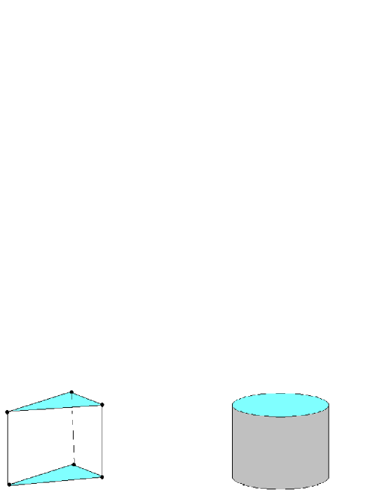
Figure 7: On left, the real skeleton of the toric web-diagram of the fibration of $O\left(-3\right)\rightarrow E^{\left(t,\infty\right)}$. It could be interpreted as a triangulation of the cylinder of base $E^{\left(t,\mathrm{\mu}\right)}$, given by the boundary of a triangle, and a non compact line as a fiber. On right, the usual cylinder $R\times S^{1}$.

The $\widetilde{Y}_{2}$ divisor of $H_{3}$ is made of the union of three sheets O$\left(-3\right)\rightarrow\mathbb{P}_{i}^{1}$ belonging to three different $\mathbb{C}^{3}$ spaces of the ambient $\mathbb{C}^{4}$.
From eqs(3.13) and (3.14), it is clear that the elliptic curve $E^{\left(t,\infty\right)}$ is an intersecting curve of the complex surfaces $Y_{2}$ and $\widetilde{Y}_{2}$.

3.3 Topological partition function

To build the non planar 3-vertex formalism for the local elliptic curve $H_{3}$, we will follow the construction used in the derivation of the usual topological 3-vertex method [28].
However since the local elliptic curve is a CY3 hypersurface in $X_{4}$,

$$H_{3}\subset X_{4},$$ (3.15)

with

$$X_{4}=\mathcal{O}(-3-m)\rightarrow WP_{1,1,1,m}^{3},$$ (3.16)

a convenient way to achieve the goal is to proceed as follows:
(1) develop the 4-vertex formalism for the ambient toric CY4-fold $X_{4}$.
(2) compute the partition function for $X_{4}$. Actually this step may be also viewed as alternative way to get the 4d generalization of the MacMahon function [50].
(3) impose the appropriate constraint relations to get the non planar 3-vertex and the topological partition function for the local elliptic curve H₃.
It is interesting to note here the emergence of a 4-vertex formalism in the construction. This is not surprising since the toric web-diagrams of $H_{3}$ and $X_{4}$ have quite similar skeletons. In the first case the tetrahedron is hollow and in the second it is full.

The first step to realize these objectives is specify the special lagrangian fibration of the toric CY4-fold like $X_{4}\sim R^{4}\times F_{4}$ with fiber taken as

$$F_{4}\sim R\times T^{3}.$$ (3.17)

On the hypersurface $H_{3}$ in $X_{4}$, real 1-cycles of $F_{4}$ shrink and one is left with the usual special lagrangian fibration of the toric CY3-folds $H_{3}\sim R^{3}\times F_{3}$ with

$$F_{3}\sim R\times T^{2}.$$ (3.18)

In [49], we give the explicit expressions of the various hamiltonians and the values of the vertices of the web-diagrams solving the Calabi-Yau conditions.
The next step is to study the 4-vertex formalism of $X_{4}$ and its reduction down to the toric hypersurface $H_{3}$.

3.3.1 Toric web-diagrams and generalized partitions

The toric web-diagrams of $X_{4}$ and $H_{3}$ have been described above (figure 5). For the case $X_{4}$, the toric web-diagram can be decomposed into four local patches

$$\mathcal{U}_{1},\quad\mathcal{U}_{2},\quad\mathcal{U}_{3},\quad\mathcal{U}_{4}.$$ (3.19)

To each patch $\mathcal{U}_{i}\sim\mathbb{C}^{4}$ with fibration $R^{4}\times F_{4}$ it is associated a topological 4-vertex $\mathcal{C}_{\left(4\right)}$. This vertex depends on the boundary conditions on its external legs. We will see that, using 3d generalized Young diagrams, it can be either defined as

$$\mathcal{C}_{\left(4\right)}=C_{\mathrm{\Lambda\Sigma\Upsilon\Gamma}},$$ (3.20)

or equivalently by using 2d partition like

$$\mathcal{C}_{\left(4\right)}=\mathcal{C}_{\left(\mathrm{\alpha\beta\gamma}\right)\left(\mathrm{\delta\epsilon\varepsilon}\right)\left(\mathrm{\zeta\eta\theta}\right)\left(\mathrm{\lambda\mu\nu}\right)}.$$ (3.21)

The toric web-diagram of $H_{3}$ is induced from the one of $X_{4}$. It can be also decomposed into four local patches as follows,

$$\mathcal{U}_{1}^{\ast},\quad\mathcal{U}_{2}^{\ast},\quad\mathcal{U}_{3}^{\ast},\quad\mathcal{U}_{4}^{\ast},$$ (3.22)

where the asterix refers to the projection

$$\ast:X_{4}\rightarrow H_{3},\qquad\mathcal{U}_{i}\rightarrow\mathcal{U}_{i}^{\ast}.$$ (3.23)

To each patch $\mathcal{U}_{i}^{\ast}\sim\mathbb{C}^{3}$ with fibration $R^{3}\times F_{3}$ it is associated a non planar topological 3-vertex $\mathcal{C}_{\left(3\right)}^{\ast},$

$$\ast:\mathcal{C}_{\left(4\right)}\rightarrow\mathcal{C}_{\left(3\right)}^{\ast}.$$ (3.24)

To get the 4- vertex $C_{\left(4\right)}$, the partition function $Z_{X_{4}}$ and the topological partition function $Z_{H_{3}}$ of the local elliptic curve, we need first introducing some key tools.
In the standard 3-vertex formalism of [28, 30], one uses a set of basic objects; in particular 2d- and 3d- partitions. In the 4-vertex formalism, we have to build the analogue of these mathematical ingredients.

$\mathbf{\alpha}$) 3d partitions

Roughly, a 3d partition $\Pi$ can be thought of as an integral $N_{1}\times N_{2}$ rank two tensor $\left(\Pi_{ia}\right)$ with the property,

$$\Pi=\left\{\Pi_{i,a}\in\mathbb{Z}_{+},\qquad\Pi_{i,a}\geq\Pi_{i+j,a+b}\geq 0\right\},$$ (3.25)

where $i,$ $j=1,2,...,N_{1}$ and $a,$ $b=1,2,...,N_{2}$.
The 3d partition, which has been used for various purposes, has a set of remarkable combinatorial features. Below, we give useful ones.
(i) 3d partitions are generalizations of the usual 2d partitions $\lambda=\left(\lambda_{1},\lambda_{2},...\right)$ with $\lambda_{1}\geq\lambda_{2}\geq....\geq 0$ and the integers $\lambda_{i}\in\mathbb{Z}_{+}$.
By setting $N_{3}=\Pi_{1,1}$, the 3d partitions can be imagined as a cubic sublattice of $\mathbb{Z}_{+}^{3}$

$$\left[1,N_{1}\right]\times\left[1,N_{2}\right]\times\left[1,N_{3}\right].$$ (3.26)

The cubic diagram of $\Pi$ can be considered as a set of unit cubes $\left(i,j,k\right)$ with integer coordinates such that $\left(i,j\right)\in\lambda$ and $1\leq k\leq\Pi(i,j)$. The integers $\Pi(i,j)$ define the height of the stack of cubes on the $\left(x_{1},x_{2}\right)$ plane. The projection of $\Pi$ on the $\left(x_{1},x_{2}\right)$ plane is just the 2d partition $\lambda$.
(ii) A subclass of 3d partitions solving the conditions (3.25) is given by the particular representation

$$\Pi=\lambda\otimes\mu,\qquad\Pi_{ia}=\lambda_{i}\mu_{a},\qquad\lambda_{i}\mu_{a}\geq\lambda_{i+j}\mu_{a+b},$$ (3.27)

where $\lambda$ and $\mu$ are 2d partitions as in eq(2.1).
We also have the following associated ones:

$$\Pi^{\text{{\small T}}}=\lambda^{\text{{\small T}}}\otimes\mu,\qquad\widetilde{\Pi}=\lambda\otimes\mu^{\text{{\small T}}},\qquad\widetilde{\Pi^{\text{{\small T}}}}=\lambda^{\text{{\small T}}}\otimes\mu^{\text{{\small T}}},$$ (3.28)

where $\lambda^{\text{{\small T}}}$ stands for the usual transpose of the Young diagram $\lambda$.
(iii) Like in the case of 2d partitions, one may associate to each 3d partition $\Pi$ a Fock space state $\left|\Pi_{ia}\right\rangle$ with norm $\left\langle\Pi|\Pi\right\rangle\equiv\left\|\Pi\right\|^{2}$,

$$\left\|\Pi\right\|^{2}=\sum_{i\geq 1}\left(\sum_{a\geq 1}\left(\Pi_{ia}\right)^{2}\right)=\sum_{a\geq 1}\left(\sum_{i\geq 1}\left(\Pi_{ia}\right)^{2}\right).$$ (3.29)

$\left\langle\Pi_{ia}\right|$ stands for the dual state associated with the dual partition $\Pi^{\mathrm{+}}=\widetilde{\Pi^{\text{{\small T}}}}$. We also have the following relation

$$I_{id}=\sum_{3d\text{ partitions}}\left|\Pi_{ia}\right\rangle\left\langle\Pi_{ia}\right|,\qquad\left\langle\Pi_{ia}|\Pi_{jb}\right\rangle=\delta_{ij}\delta_{ab},$$ (3.30)

defining the resolution of the identity operator $I_{id}$.
(iv) The number $\left|\Pi\right|$ of unit boxes (cubes) of the 3d partition is defined as

$$\left|\Pi\right|=\sum_{i,a}\Pi_{i,a}.$$ (3.31)

(v) The boundary $\left(\partial\Pi\right)$ of the 3d partition $\Pi$ is given by the 2d profile of the corresponding generalized Young diagram. As this property is important for the present study, let give some details.
Given a 3d partition $\Pi$, the boundary term on the plane $x_{i}=N_{i}$ is a Young diagram (2d partition). On the planes $x_{1}=N_{1}$, $x_{2}=N_{2}$ and $x_{3}=N_{3}$, the boundary of $\Pi$ is composed of by three 2d partitions $\lambda,$ $\mu$ and $\nu$. So we then have:

$$\partial\Pi=\left(\lambda,\mu,\nu\right).$$ (3.32)

Particular boundaries are given by the case where a 2d partition is located at infinity; that is there is no boundary. We distinguish the following situations:

$$\partial\Pi = \left(\emptyset,\mu,\nu\right),$$

$$\partial\Pi = \left(\emptyset,\emptyset,\nu\right),$$ (3.33)

$$\partial\Pi = \left(\emptyset,\emptyset,\emptyset\right),$$

where $\emptyset$ stands for the vacuum.
(vi) A convenient way to deal with 3d partitions is to slice them as a sequence of 2d partitions with interlacing relations. We mainly distinguish two kinds of sequences of 2d partitions: perpendicular and diagonal. We will not need this property here; but for details on this matter see for instance [30] and refs therein.

$\mathbf{\beta}$) 4d partitions

The 4d partitions $\mathcal{P}$ are extensions of the 3d partitions $\Pi$ considered above. They can be imagined as 4d generalized Young diagrams described by the typical integral rank 3- tensor ,

$$\mathcal{P}_{ia\alpha}\in\mathbb{Z}_{+},\qquad\text{with\qquad}\mathcal{P}_{ia\alpha}\geq\mathcal{P}_{\left(i+j\right)\left(a+b\right)\left(\alpha+\beta\right)},\quad$$ (3.34)

with $1\leq i\leq N_{1},$ $1\leq a\leq N_{2}$ and $1\leq\alpha\leq N_{3}$.
Several properties of 2d and 3d partitions extend to the 4d case; there are also specific properties in particular those concerning their slicing into lower dimensional ones. Below we describe some particular properties of 4d partitions by considering special representations.
Sub-classes of 4d partitions are given by:
(i) the product of a 2d- and a 3d- partitions $\mu$ and $\Pi$ like

$$\mathcal{P}=\mu\otimes\Pi,\qquad\left(\mathcal{P}_{ia\alpha}\right)=\left(\mu_{i}\Pi_{a\alpha}\right),$$ (3.35)

with $i=1,...,N_{1}$; $a=1,...,N_{2}$ and $\alpha=1,...,N_{3}$.
(ii) the product of three kinds of 2d- partitions.

$$\mathcal{P}=\lambda\otimes\mu\otimes\nu,\qquad\left(\mathcal{P}_{ia\alpha}\right)=\left(\lambda_{i}\mu_{a}\nu_{\alpha}\right).$$ (3.36)

The boundary $\partial\mathcal{P}$ of a generic 4d partition $\mathcal{P}$ can be defined in two ways. First in terms of 3d partitions as follows

$$\partial\mathcal{P}=\left(\Lambda,\Pi,\Sigma,\Upsilon\right).$$ (3.37)

We also have the following particular boundary conditions

case I $$: \partial\mathcal{P}=\left(\varnothing,\Pi,\Sigma,\Upsilon\right),$$

case II $$: \partial\mathcal{P}=\left(\varnothing,\varnothing,\Sigma,\Upsilon\right),$$

case III $$: \partial\mathcal{P}=\left(\varnothing,\varnothing,\varnothing,\Upsilon\right),$$ (3.38)

case IV $$: \partial\mathcal{P}=\left(\varnothing,\varnothing,\varnothing,\varnothing\right),$$

where $\varnothing$ stands for the the ”3d vacuum” (no boundary condition).
Second by using 2d partitions to define boundary of $\mathcal{P}$ like

$$\partial\mathcal{P}=\left(\text{ }\left[\mathrm{a,b,c}\right];\text{ \ }\left[\mathrm{d,e,f}\right];\text{ }\left[\mathrm{g,h,i}\right];\text{ }\left[\mathrm{j,k,l}\right]\text{ \ }\right),$$ (3.39)

where $\left[\mathrm{abc}\right]$, …and $\left[\mathrm{jkl}\right]$ stand for the boundaries of the 3d partitions $\Lambda,...$ and $\Upsilon$.
Notice that the second representation is more richer since along with the configuration

$$\varnothing=\left[\emptyset,\emptyset,\emptyset\right],$$ (3.40)

we have moreover the two following extra configurations

$$\left[\mathrm{\emptyset,b,c}\right],\qquad\left[\mathrm{\emptyset,\emptyset,c}\right].$$ (3.41)

For the case I of eq(3.38) corresponds then the three following boundary configurations

$$\partial\mathcal{P}=\left\{\begin{array}[]{c}\text{case i}:\qquad\left(\left[\mathrm{\emptyset,b,c}\right];\text{\quad}\left[\mathrm{d,e,f}\right];\text{\quad}\left[\mathrm{g,h,i}\right];\text{\quad}\left[\mathrm{j,k,l}\right]\right)\\ \\ \text{case ii}:\qquad\left(\left[\mathrm{\emptyset,\emptyset,c}\right];\text{\quad}\left[\mathrm{d,e,f}\right];\text{\quad}\left[\mathrm{g,h,i}\right];\text{\quad}\left[\mathrm{j,k,l}\right]\right)\\ \\ \text{case iii}:\qquad\left(\left[\mathrm{\emptyset,\emptyset,\emptyset}\right];\text{\quad}\left[\mathrm{d,e,f}\right];\text{\quad}\left[\mathrm{g,h,i}\right];\text{\quad}\left[\mathrm{j,k,l}\right]\right)\end{array}\right|,$$ (3.42)

where the last one (case iii) is the case I described by the first relation of eq(3.38).
This property indicates that one disposes of different ways to deal with 4d partitions either the simplest one using 3d-partitions or the more refined on involving 2d partitions. Below we consider both representations.

Notice moreover that given a 4d partition $\mathcal{P}$, we can associate to it various kinds of transpose partitions. Using the particular realization eq(3.36), the corresponding transposes read as

$$\lambda^{\mathrm{T}}\otimes\mu\otimes\nu,\qquad\lambda\otimes\mu^{\mathrm{T}}\otimes\nu,\qquad\lambda\otimes\mu\otimes\nu^{\mathrm{T}},$$

$$\lambda^{\mathrm{T}}\otimes\mu^{\mathrm{T}}\otimes\nu,\qquad\lambda\otimes\mu^{\mathrm{T}}\otimes\nu^{\mathrm{T}},\qquad\lambda^{\mathrm{T}}\otimes\mu\otimes\nu^{\mathrm{T}},$$ (3.43)

$$\lambda^{\mathrm{T}}\otimes\mu^{\mathrm{T}}\otimes\nu^{\mathrm{T}},$$

where $\lambda^{\mathrm{T}}$ stands for the usual transpose of the Young diagram $\lambda$.
The exact mathematical definitions and the full properties of 4d partitions are not our immediate objective here; they need by themselves a separate study. Here above we have given just the needed properties to set up the structure of the 4-vertex formalism and its restricted non planar 3-vertex method.

3.3.2 Tetra- vertex $C_{\left(4\right)}$ and $Z_{X_{4}}$

$\mathbf{\alpha}$) the 4- vertex $C_{\left(4\right)}$

The 4- vertex $C_{\left(4\right)}$ of the toric Calabi-Yau X₄ can be built by extending the 3-vertex construction eq(2.3).

In the 3d partition set up, the vertex $\mathcal{C}_{\left(4\right)}$ has four external legs $L_{\Lambda},L_{\Sigma},L_{\Upsilon},L_{\Gamma}$ with boundary conditions as in eq(3.37). The 4-vertex $\mathcal{C}_{\left(4\right)}$ with boundary conditions $\left(\Lambda\Sigma\Upsilon\Gamma\right)$ can be defined as a function of the Bolzmann weight $q=e^{-\beta}$ as follows:

$$\mathcal{C}_{\Lambda\Sigma\Upsilon\Gamma}\equiv\mathcal{C}_{\Lambda\Sigma\Upsilon\Gamma}\left(q\right).$$ (3.44)

In the case where $\Lambda=\Sigma=\Upsilon=\Gamma=\varnothing$, the corresponding 4- vertex $\mathcal{C}_{\varnothing\varnothing\varnothing\varnothing}$ should be equal to the generating function $Z_{\mathbb{C}^{4}}$ of the 4d generalized Young diagrams

$$\mathcal{C}_{\varnothing\varnothing\varnothing\varnothing}=Z_{\mathbb{C}^{4}}.$$ (3.45)

Recall that the generating functional $Z_{\mathbb{C}^{4}}$ can be defined as a power series like,

$$Z_{\mathbb{C}^{4}}=\sum_{\text{4d partitions }\mathcal{P}}q^{\left|\mathcal{P}\right|},$$ (3.46)

where $\left|\mathcal{P}\right|$ is the number of hypercubes in $\mathcal{P}$.
In the generic case, $\mathcal{C}_{\Lambda\Sigma\Upsilon\Gamma}$ should be given by the generalization of the 3-vertex (2.4) and could a priori be expressed in terms of the product of some hypothetic generalized Schur functions $\mathcal{S}_{\Lambda}\left(q\right)$.

In the 2d partition set up, one can $\mathcal{C}_{\left(4\right)}$ in quite similar manner. Using eqs(3.37-3.39), we can generally define it as in eq(3.21). This is a kind of rank 12 object

$$\mathcal{C}_{\left(\mathrm{abc}\right)\left(\mathrm{def}\right)\left(\mathrm{ghi}\right)\left(\mathrm{jkl}\right)},$$ (3.47)

depending on the Boltzmann weight and the boundary conditions (external momenta) $\mathrm{a,...,l}$.
To obtain its explicit expression, we use the following
(i) the relation between the 4-vertex and composites of planar 3-vertices.
(ii) the results on the usual 3-vertex formalism.
The first property follows by noting that 4-vertices of the toric web-diagram of $X_{4}$ with the special Lagrangian fibration

$$R^{4}\times R\times T^{3},$$ (3.48)

corresponds to the intersection of the planar 3-vertices of three triangles. To fix the ideas, consider figure 5 and focus on the point A representing a 4-vertex of the toric web-diagram of X₄. The point A is the intersection

$$A=\Delta_{1}\cap\Delta_{2}\cap\Delta_{3},$$ (3.49)

of the triangles,

$$\Delta_{1} =$$ triangle ABC,

$$\Delta_{2} =$$ triangle ABD, (3.50)

$$\Delta_{3} =$$ triangle ACD,

These triangles are boundary faces of the tetrahedron

$$\text{ABCD}.$$ (3.51)

Inside of the tetrahedron, the toric fiber is

$$T^{3}=\mathbb{S}^{1}\times\mathbb{S}^{1}\times\mathbb{S}^{1}.$$ (3.52)

On each triangle face, a circle shrinks leaving $T^{2}$.
On each egde of a triangle, one more circle shrinks leaving $\mathbb{S}^{1}$.
At the vertex A, all 1-cycles of $T^{3}$ shrinks down to zero.
The property captured by eqs(3.49) means that we may relate the 4-vertex $C_{\Lambda\Sigma\Upsilon\Gamma}$ to three planar vertices of the triangles (3.50). This can be done by expressing the 3d partitions $\left(\Lambda,\Sigma,\Upsilon,\Gamma\right)$ in terms of 2d partitions $\left(\mathrm{a,b,c}\right),$ $\left(\mathrm{d,e,f}\right),$ $\left(\mathrm{g,h,i}\right)$ and $\left(\mathrm{j,k,l}\right)$ as follows

$$\Lambda = \left(\mathrm{a,d,g}\right),\qquad\Sigma=\left(\mathrm{b,c,\emptyset}\right),$$

$$\Upsilon = \left(\mathrm{e,\emptyset,f}\right),\qquad\Gamma=\left(\mathrm{\emptyset,h,i}\right).$$ (3.53)

The decomposition (3.53) is illustrated on the formal figure 8 where the three triangles are represented in different colors.

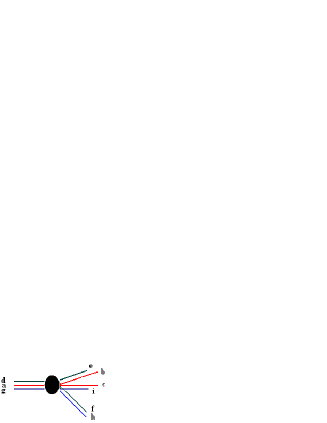
Figure 8: A typical 4-vertex in $\mathcal{O}\left(-3-m\right)\rightarrow WP_{1,1,1,m}^{3}$ using 2d partitions. This is a spatial vertex made of three planar 3-vertices: ($\mathrm{abc),(def)}$ and ($\mathrm{ghi}$).

Substituting $\left(\Lambda\Sigma\Upsilon\Gamma\right)$ as in eq(3.53), we can first rewrite $\mathcal{C}_{\Lambda\Sigma\Upsilon\Gamma}$ like $\mathcal{C}_{\left(\mathrm{adh}\right)\left(\mathrm{bc\emptyset}\right)\left(\mathrm{e\emptyset f}\right)\left(\mathrm{\emptyset hi}\right)}$. The latter reads immediately from the figure 8 and is given by

$$\mathcal{C}_{\left(\mathrm{adg}\right)\left(\mathrm{bc\emptyset}\right)\left(\mathrm{e\emptyset f}\right)\left(\mathrm{\emptyset hi}\right)}=C_{\mathrm{abc}}C_{\mathrm{def}}C_{\mathrm{ghi}},$$ (3.54)

where $C_{\mathrm{abc}}$, $C_{\mathrm{def}}$ and $C_{\mathrm{ghi}}$ are topological 3-vertices with the explicit expression eq(2.4).

$\mathbf{\beta}$) the function $Z_{X_{4}}$

The the toric web-diagram of the $X_{4}$ 4-fold is given by figure 9.

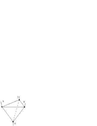
Figure 9: A typical the toric web-diagram of X₄ with boundary conditions $\left(\Lambda\Pi\Sigma\Upsilon\right).$

The corresponding partition function $Z_{X_{4}}$ can be computed by specifying the 4-vertices, propagators, framings and using Feynman like rules. Notice that in the 2d partition set up, the toric webs of $X_{4}$ and $H_{3}$ are as in the figure 10.

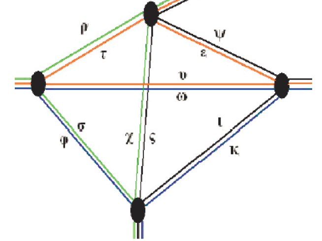
Figure 10: toric web-diagram of the local elliptic curve using 2d partitions. External and internal momenta have been expressed in terms of 2d partitions. 

Using the momenta prescriptions described by the Young diagrams of the figure 10 as well as trivial boundary conditions for the extrenal legs, the partition function reads in terms of the Kahler modulus $t$ of $X_{4}$ as follows:

$$Z_{H_{3}}=\sum_{\left\{\varkappa\right\}}\left[\left(\mathcal{A}_{\tau\nu^{\mathrm{T}}\omega\varphi^{\mathrm{T}}\rho\sigma^{\mathrm{T}}}\right)\left(\mathcal{B}_{\varepsilon\tau^{\mathrm{T}}\chi\rho^{\mathrm{T}}\psi\varsigma^{\mathrm{T}}}\right)\left(\mathcal{F}_{\upsilon\epsilon^{\mathrm{T}}\iota\psi^{\mathrm{T}}\kappa\omega^{\mathrm{T}}}\right)\left(\mathcal{G}_{\varphi\kappa^{\mathrm{T}}\chi\sigma^{\mathrm{T}}\iota\varsigma^{\mathrm{T}}}\right)\mathcal{H}_{\tau\upsilon\omega\varphi\rho\sigma\varepsilon\chi\iota\kappa\psi\varsigma}\right]$$ (3.55)

where the sum over $\left\{\varkappa\right\}$ stands for the collective sum over the 2d- partitions $\varkappa=\tau,$ $\upsilon,$ $\omega,$ $\varphi,$ $\rho,$ $\sigma,$ $\varepsilon,$ $\chi,$ $\iota,$ $\kappa,$ $\psi,$ $\varsigma$ and where we have set

$$\mathcal{A}_{\tau\upsilon^{\mathrm{T}}\omega\varphi^{\mathrm{T}}\rho\sigma^{\mathrm{T}}} = C_{\emptyset\tau\upsilon^{\mathrm{T}}}C_{\emptyset\omega\varphi^{\mathrm{T}}}C_{\emptyset\rho\sigma^{\mathrm{T}}},$$

$$\mathcal{B}_{\varepsilon\tau^{\mathrm{T}}\chi\rho^{\mathrm{T}}\psi\varsigma^{\mathrm{T}}} = C_{\emptyset\varepsilon\tau^{\mathrm{T}}}C_{\emptyset\chi\rho^{\mathrm{T}}}C_{\emptyset\psi\varsigma^{\mathrm{T}}},$$

$$\mathcal{F}_{\upsilon\varepsilon^{\mathrm{T}}\iota\psi^{\mathrm{T}}\kappa\omega^{\mathrm{T}}} = C_{\emptyset\upsilon\varepsilon^{\mathrm{T}}}C_{\emptyset\iota\psi^{\mathrm{T}}}C_{\emptyset\kappa\omega^{\mathrm{T}}},$$ (3.56)

$$\mathcal{G}_{\varphi\kappa^{\mathrm{T}}\chi\sigma^{\mathrm{T}}\iota\varsigma^{\mathrm{T}}} = C_{\emptyset\varphi\kappa^{\mathrm{T}}}C_{\emptyset\chi\sigma^{\mathrm{T}}}C_{\emptyset\iota\varsigma^{\mathrm{T}}},$$

and

$$\mathcal{H}_{\tau\upsilon\omega\varphi\rho\sigma\varepsilon\chi\iota\kappa\psi\varsigma}=\mathop{\displaystyle\prod}\limits_{\varkappa=\tau,\upsilon,\omega,\varphi,\rho,\sigma,\varepsilon,\chi,\iota,\kappa,\psi,\varsigma}(-e^{-t})^{\left|\varkappa\right|}q^{\kappa\left(\varkappa\right)},$$ (3.57)

where $\kappa\left(\mu\right)$ is the second Casimir of the 2d partition $\mu$ (2.8). The factors $C_{\alpha\beta\gamma}$ are given by eq(2.4)

3.3.3 Partition function for the local 2-torus

The partition function $Z_{H_{3}}$ of the local elliptic curve may be obtained by implementing in $Z_{X_{4}}$ the constraint relations (3.24) capturing the projection $X_{4}\rightarrow H_{3}$.
Choosing trivial boundary conditions for the external legs and using:
(i) the expression of the 4-vertex (3.54),
(ii) the rules of the planar vertex formalism of [28],
we can write down directly the expression of the partition function $Z_{H_{3}}$. We find

$$Z_{H_{3}}=\sum_{\xi,\rho,\sigma,\eta,\upsilon,\tau,\varsigma,\theta}\left(\mathcal{A}_{\omega\varphi^{\mathrm{T}}\rho\sigma^{\mathrm{T}}}^{\ast}\mathcal{B}_{\chi\rho^{\mathrm{T}}\psi\varsigma^{\mathrm{T}}}^{\ast}\mathcal{F}_{\iota\psi^{\mathrm{T}}\kappa\omega^{\mathrm{T}}}^{\ast}\mathcal{G}_{\varphi\kappa^{\mathrm{T}}\chi\sigma^{\mathrm{T}}\iota\varsigma^{\mathrm{T}}}^{\ast}\mathcal{H}_{\omega\varphi\rho\sigma\chi\iota\kappa\psi\varsigma}^{\ast}\right),$$ (3.58)

with

$$\mathcal{A}_{\omega\varphi^{\mathrm{T}}\rho\sigma^{\mathrm{T}}}^{\ast} = C_{\emptyset\omega\varphi^{\mathrm{T}}}C_{\emptyset\rho\sigma^{\mathrm{T}}},$$

$$\mathcal{B}_{\chi\rho^{\mathrm{T}}\psi\varsigma^{\mathrm{T}}}^{\ast} = C_{\emptyset\chi\rho^{\mathrm{T}}}C_{\emptyset\psi\varsigma^{\mathrm{T}}},$$

$$\mathcal{F}_{\iota\psi^{\mathrm{T}}\kappa\omega^{\mathrm{T}}}^{\ast} = C_{\emptyset\iota\psi^{\mathrm{T}}}C_{\emptyset\kappa\omega^{\mathrm{T}}},$$ (3.59)

$$\mathcal{G}_{\varphi\kappa^{\mathrm{T}}\chi\sigma^{\mathrm{T}}\iota\varsigma^{\mathrm{T}}}^{\ast} = C_{\emptyset\varphi\kappa^{\mathrm{T}}}C_{\emptyset\chi\sigma^{\mathrm{T}}}C_{\emptyset\iota\varsigma^{\mathrm{T}}},,$$

together with

$$\mathcal{H}_{\omega\varphi\rho\sigma\chi\iota\kappa\psi\varsigma}^{\ast}=\mathop{\displaystyle\prod}\limits_{\mu=\left\{\omega,\varphi,\rho,\sigma,\chi,\iota,\kappa,\psi,\varsigma\right\}}(-e^{-t})^{\left|\mu\right|}q^{\kappa\left(\mu\right)}$$ (3.60)

where the factors $C_{\alpha\beta\gamma}$ are as in eq(2.4).
In what follows, we turn to study the field theory set up of the local 2-torus by starting by local $\mathbb{P}^{2}$ model.

4 Sigma model for local $\mathbb{P}^{2}$

In this section, we first review briefly the supersymmetric sigma linear model realization of the local $\mathbb{P}^{2}$ model. This model is useful for the purpose of this paper.
We also use this field realization to fix convention notations and to introduce some mathematical objects and their physical interpretations.

The local $\mathbb{P}^{2}$ model is nicely formulated in the language of $4D$, $\mathcal{N}=1$ supersymmetry which is, roughly, equivalent to the usual $2D$, $\mathcal{N}=2$ supersymmetry. The complex two dimension projective plane $\mathbb{P}^{2}$ has one Kahler parameter $t$, interpreted as the Fayet-Iliopoulos (FI) coupling constant in the supersymmetric gauge theory.
The $U\left(1\right)$ gauged linear sigma theory describing the local $\mathbb{P}^{2}$ target space geometry involves the following $4D$, $\mathcal{N}=1$ superfields (supersymmetric representations):
(1) A $U\left(1\right)$ gauge superfield $V=V\left(x,\theta,\overline{\theta}\right)$ which reads, in the Wess-Zumino gauge, as follows:

$$V=-\theta\sigma^{\mu}\overline{\theta}A_{\mu}-i\overline{\theta}^{2}\theta\lambda+i\theta^{2}\overline{\theta}\overline{\lambda}+\frac{1}{2}\theta^{2}\overline{\theta}^{2}D,$$ (4.1)

where $\left(x^{\mu},\theta^{a},\overline{\theta}_{\dot{a}}\right)$ stands for the $4D$, $\mathcal{N}=1$ superspace coordinates.
In this relation, $A_{\mu}\left(x\right)$ and $\left(\lambda_{a}\left(x\right),\overline{\lambda}_{\dot{a}}\left(x\right)\right)$ are respectively the $U\left(1\right)$ gauge vector and gaugino fields.
The scalar field $D$ is the usual auxiliary field capturing the local Calabi-Yau geometry. It captures as well as part of the scalar field potential $V$ of the gauge theory

$$V=D^{2}+\sum_{i}\left|F_{i}\right|^{2},$$ (4.2)

where the $F_{i}$ terms will be introduced below.
(2) Four chiral superfields $\left\{\Phi_{0},\Phi_{1},\Phi_{2},\Phi_{3}\right\}$, with $\theta$-expansion

$$\Phi_{i}=z_{i}+\theta\psi_{i}+\theta^{2}F_{i},$$ (4.3)

with $z_{i}$ being the field coordinates of local $\mathbb{P}^{2}$, $\psi_{i}$ the Weyl spinors and $F_{i}$ the so called F-auxiliary fields.
The $\Phi_{i}$ complex superfields carry the following $q_{i}$- charges under the $U\left(1\right)$ gauge symmetry,

$$\left(q_{0},q_{1},q_{2},q_{3}\right)=\left(-3,1,1,1\right).$$ (4.4)

The $q_{i}$’s add exactly to zero as required by the Calabi-Yau condition

$$\sum_{i=0}^{3}q_{i}=0,$$ (4.5)

of local $\mathbb{P}^{2}$.
The superfield Lagrangian density $\mathcal{L}_{\text{local }P^{2}}=\mathcal{L}\left(\Phi,V\right)$ of the local $\mathbb{P}^{2}$ model reads, in the $\mathcal{N}=1$ $D=4$ formalism, as follows,

$$\mathcal{L}\left(\Phi,V\right)=\int d^{4}\theta\sum_{i=0}^{3}\overline{\Phi}_{i}e^{2q_{i}V}\Phi_{i}-2t\int d^{4}\theta V+\mathcal{L}_{{\small gauge}}\left(V\right).$$ (4.6)

Here $\mathcal{L}_{gauge}\left(V\right)$ is the superspace Lagrangian density for the $U\left(1\right)$ vector multiplet that can be found in [47]. The equation of motion of the auxiliary field D leads to,

$$\left|z_{1}\right|^{2}+\left|z_{2}\right|^{2}+\left|z_{3}\right|^{2}-3\left|z_{0}\right|^{2}=t.$$ (4.7)

It is nothing but the defining equation of the local projective plane $\mathcal{O}\left(-3\right)\rightarrow\mathbb{P}^{2}$.
The compact part $\mathbb{P}^{2}$ of this threefold is a complex plane given by the divisor $z_{0}=0$; it is parameterized by the complex coordinates $\left(z_{1},z_{2},z_{3}\right)$ describing a complex surface embedded in $\mathbb{C}^{3}$ and has a $U\left(1\right)$ gauge symmetry rotating the phases of the coordinates variables.
By setting $x_{i}=\left|z_{i}\right|^{2}$, the complex surface $z_{0}=0$ can be represented by the planar triangle [48],

$$x_{1}+x_{2}+x_{3}=t$$ (4.8)

with Kahler modulus $t$; see also figure 1.
Because of the symmetry under permutation of the $x_{i}$’s, the triangle is equilateral. The length of its edges are equal to $t$ and then it has an area given by $A=\frac{t^{2}\sqrt{3}}{2}$.

5 Field model for $\mathcal{O}\left(-3\right)\rightarrow E^{\left(t,\infty\right)}$

We first study the gauge invariant supersymmetric field model with target space given by the curve $E^{\left(t,\infty\right)}=\partial\mathbb{P}^{2}$. For details on the degenerate elliptic curve $E^{\left(t,\infty\right)}$, see the appendix. Then, we consider the extension to $O\left(-3\right)\rightarrow E^{\left(t,\infty\right)}$.

5.1 Divisors of local $\mathbb{P}^{2}$

To begin, notice that the local $\mathbb{P}^{2}$ eq(4.7) has several divisors; i.e codimension one subspaces describing boundary patches of the normal bundle of the projective plane.
The standard ones are obtained by setting one of the $z_{i}$’s to zero; $z_{i}=0$ with $i=0,1,2,3$.

5.1.1 Toric boundary of $\mathbb{P}^{2}$

In this paragraph, we consider the three following complex surfaces $\left[D_{1}\right]$, $\left[D_{2}\right]$ and $\left[D_{3}\right]$,

$$\left[D_{1}\right] : \left|z_{2}\right|^{2}+\left|z_{3}\right|^{2}-3\left|z_{0}\right|^{2}=t,\qquad\Leftrightarrow\qquad z_{1}=0,$$

$$\left[D_{2}\right] : \left|z_{3}\right|^{2}+\left|z_{1}\right|^{2}-3\left|z_{0}\right|^{2}=t,\qquad\Leftrightarrow\qquad z_{2}=0,$$ (5.1)

$$\left[D_{3}\right] : \left|z_{1}\right|^{2}+\left|z_{2}\right|^{2}-3\left|z_{0}\right|^{2}=t,\qquad\Leftrightarrow\qquad z_{3}=0,$$

and their union $\left[D\right]=\left[D_{1}\right]\cup\left[D_{2}\right]\cup\left[D_{3}\right]$.
To see what this local geometry describes precisely; let us set $\left|z_{0}\right|^{2}=0$ in above eqs from where one sees that each relation describes a complex one dimension projective line $\mathbb{P}^{1}$. To distinguish between these complex projective lines, we use the convention notation $\mathbb{P}_{i}^{1}$ where the subindex $i$ refers to $z_{i}=0$. Thus we have

$$\mathbb{P}_{1}^{1} : \left|z_{2}\right|^{2}+\left|z_{3}\right|^{2}=t,$$

$$\mathbb{P}_{2}^{1} : \left|z_{3}\right|^{2}+\left|z_{1}\right|^{2}=t,$$ (5.2)

$$\mathbb{P}_{3}^{1} : \left|z_{1}\right|^{2}+\left|z_{2}\right|^{2}=t.$$

As we see, these projective lines have the following intersection matrix

$$\mathbb{P}_{i}^{1}\cap\mathbb{P}_{j}^{1}=\left(\begin{array}[]{ccc}-2&1&1\\ 1&-2&1\\ 1&1&-2\end{array}\right),$$ (5.3)

from which one sees that the complex curve

$$E^{\left(t,\infty\right)}=\mathbb{P}_{1}^{1}\cup\mathbb{P}_{2}^{1}\cup\mathbb{P}_{3}^{1},$$ (5.4)

is elliptic ($E^{\left(t,\infty\right)}\sim\mathbb{T}^{2}$). Indeed, computing

$$E^{\left(t,\infty\right)}\cap E^{\left(t,\infty\right)}=\sum_{i=1}^{3}\mathbb{P}_{i}^{1}\cap\mathbb{P}_{i}^{1}+2\left(\mathbb{P}_{1}^{1}\cap\mathbb{P}_{2}^{1}+\mathbb{P}_{2}^{1}\cap\mathbb{P}_{3}^{1}+\mathbb{P}_{3}^{1}\cap\mathbb{P}_{1}^{1}\right),$$ (5.5)

we get, up on using (5.3),

$$E^{\left(t,\infty\right)}\cap E^{\left(t,\infty\right)}=-3\times 2+2\times 3=0.$$ (5.6)

From the toric diagram of $\mathbb{P}^{2}$, one also see that $E^{\left(t,\infty\right)}$ describes indeed a toric complex one dimensional curve defining the toric boundary of $\mathbb{P}^{2}$; i.e:

$$E^{\left(t,\infty\right)}\equiv\partial\mathbb{P}^{2}.$$ (5.7)

It is this curve that will be used to deal with the local 2-torus in the large complex structure limit.

5.1.2 Elliptic curve $E^{\left(t,\infty\right)}$

An interesting question concerns the derivation of the defining equation describing the elliptic curve $E^{\left(t,\infty\right)}$. From the above analysis, it is not difficult to see that $E^{\left(t,\infty\right)}$ is given by the following system of equations,

$$\left\{\begin{array}[]{c}\left|z_{1}\right|^{2}+\left|z_{2}\right|^{2}+\left|z_{3}\right|^{2}=t\\ z_{i}\equiv z_{i}e^{iq_{i}\alpha},\\ z_{1}z_{2}z_{3}=0.\end{array}\right.$$ (5.8)

In these relations, we have three complex variables $\left(z_{1},z_{2},z_{3}\right)$ subject to three constraint eqs,

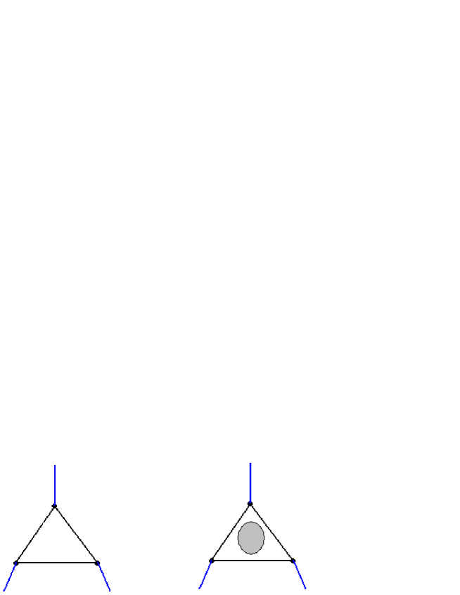
Figure 11: (a) Left: Toric graph of $\mathbb{P}^{2}$. (b) Right: toric graph of E^(t,∞) where we have added a hole to avoid confusion.

The two first eqs, which are real, are just the defining linear sigma model eq of $\mathbb{P}^{2}$. They will be interpreted as the field equation of motion of the auxiliary D- field in supersymmetric sigma model.
The third relation, which is covariant under $U\left(1\right)$ gauge symmetry, is an extra complex condition implemented in order to restrict $\mathbb{P}^{2}$ geometry to its toric boundary $\partial\mathbb{P}^{2}$. It will be interpreted later as the equation of motion of the auxiliary F- fields.
Notice that, the implementation of the boundary condition is a new feature. It can be then viewed as:
(i) a generalization of the usual approach for dealing with sigma model realization of toric manifolds.
(ii) a way to approach genus g Riemann surfaces.
(iii) a method that can be used to describe the toric boundary of more general complex n dimensional toric Calabi-Yau manifolds. We will make a comment regarding this point in the conclusion section.
Notice finally that for $t\neq 0$ the three complex variables cannot vanish simultaneously, i.e

$$\left(z_{1},z_{2},z_{3}\right)\neq\left(0,0,0\right)$$ (5.9)

In the particular case $t=0$, the geometry collapses to the origin $\left(0,0,0\right)$ where live a $\mathbb{P}^{2}$ singularity and an elliptic one.

5.1.3 Divisor $\mathcal{O}\left(-3\right)\rightarrow E^{\left(t,\infty\right)}$

Using the above result on the toric realization of the elliptic curve, one can immediately write down the defining equation of the divisor $\mathcal{O}\left(-3\right)\rightarrow E^{\left(t,\infty\right)}$ of the local $\mathbb{P}^{2}$. We have

$$\left\{\begin{array}[]{c}\left|z_{1}\right|^{2}+\left|z_{2}\right|^{2}+\left|z_{3}\right|^{2}-3\left|z_{0}\right|^{2}=t\\ z_{i}\equiv z_{i}e^{iq_{i}\alpha},\qquad i=0,1,2,3,\\ z_{1}z_{2}z_{3}=0,\end{array}\right.$$ (5.10)

where $\left(q_{0},q_{1},q_{2},q_{3}\right)$ are as in eq(4.4) and where the complex variable $z_{0}$ parameterizes the non compact direction $\mathcal{O}\left(-3\right)$.
If we do not worry about the Calabi-Yau condition, the first relation can be extended as

$$\left|z_{1}\right|^{2}+\left|z_{2}\right|^{2}+\left|z_{3}\right|^{2}-m\left|z_{0}\right|^{2}=t.$$ (5.11)

where $m$ is an arbitrary positive integer.

5.2 Superfield action

Here we give the supersymmetric field description of (5.11). We start by studying the field realization of the toric curve $E^{\left(t,\infty\right)}$. Then we consider its extension to the local geometry.

5.2.1 Gauge invariant model for the elliptic curve

To build the supersymmetric model describing the toric curve $E^{\left(t,\infty\right)}$, we start from the superfield content eq(4.7) of local $\mathbb{P}^{2}$ theory and implement the constraint equation (5.10) by using Lagrange multiplier method together $U\left(1\right)$ gauge invariance.
The appropriate Lagrange superfield multiplier is given by a chiral superfield $\Upsilon$ with charge $q_{\Upsilon}=-3$ under $U\left(1\right)$ gauge symmetry so that the chiral superfield monomial

$$W\left(\Phi,\Upsilon\right)=\Phi_{1}\Phi_{2}\Phi_{3}\Upsilon,$$ (5.12)

is gauge invariant. Thus the supersymmetric Lagrangian super-density with target space $E^{\left(t,\infty\right)}$ is given by the density,

$$\mathcal{L}_{{\small E}}=\mathcal{L}_{P^{2}}+\left(g\int d^{2}\theta W\left(\Phi,\Upsilon\right)+hc\right),$$ (5.13)

where $g$ is a complex coupling constant. Since $\Upsilon$ has no kinetic term, its elimination through the equation of motion

$$\frac{\delta\mathcal{L}_{{\small E}}}{\delta\Upsilon}=0$$ (5.14)

gives

$$g\Phi_{1}\Phi_{2}\Phi_{3}=0,$$ (5.15)

whose lowest term is precisely $z_{1}z_{2}z_{3}=0$.
Notice that contrary to $\mathbb{P}^{2}$, the superfield realization of the curve $E^{\left(t,\infty\right)}$ has a non trivial chiral superpotential. As we see, this result is a particular situation that can be extended to build toric realization of other toric manifolds.
Notice also that the Lagrange superfield multiplier $\Upsilon$ can be given a geometric interpretation. This superfield has no kinetic term $\overline{\Upsilon}\Upsilon$ nor couplings to the gauge superfield $V$; i.e no term type

$$\int d^{4}\theta\overline{\Upsilon}e^{2qV}\Upsilon,$$ (5.16)

in the Lagrangian super-density. The lack of (5.16) can be interpreted as corresponding to freezing the supersymmetric gauge invariant dynamics of $\Upsilon$. This property explains why the Calabi-Yau condition for the complex toric curve $E^{\left(t,\infty\right)}$ should read as,

$$\sum_{i=1}^{3}q_{i}+q_{\gamma}=\sum_{i=1}^{3}q_{i}-3=0.$$ (5.17)

We will turn to this property when we consider the local threefold $\mathcal{O}\left(m\right)\oplus\mathcal{O}\left(-m\right)\rightarrow E^{\left(t,\infty\right)}$.
Notice also that the chiral superpotential (5.12) is not the unique gauge invariant term one may have. The general form of $W\left(\Phi,\Upsilon\right)$ is given by

$$W\left(\Phi,\Upsilon\right)=\sum_{n_{1}+n_{2}+n_{3}=3}\mathrm{g}_{{\small n}_{1}{\small,n}_{2}{\small,n}_{3}}\Phi_{1}^{n_{1}}\Phi_{2}^{n_{2}}\Phi_{3}^{n_{3}}.$$ (5.18)

We will discuss this point in section 5 when we study the generalization to higher dimension CY manifolds.
For the moment, let us complete this discussion by giving the gauged superfield realization of the complex surface $\mathcal{O}\left(-m\right)\rightarrow E^{\left(t,\infty\right)}$.

5.2.2 Field model for the Divisor $\mathcal{O}\left(-m\right)\rightarrow E^{\left(t,\infty\right)}$

In addition to the $U\left(1\right)$ gauge superfield $V$, this model involves five chiral superfields $\left(\Phi_{0},\Phi_{1},\Phi_{2},\Phi_{3},\Upsilon\right)$ with charges

$$\left(q_{0},q_{1},q_{2},q_{3},q_{\gamma}\right)=\left(-m,1,1,1,-3\right).$$ (5.19)

The Lagrangian super-density $\mathcal{L}_{divisor}$ is given by,

$$\mathcal{L}_{{\small divisor}} = \int d^{4}\theta\sum_{i=0}^{3}\overline{\Phi}_{i}e^{2q_{i}V}\Phi_{i}+\mathcal{L}_{{\small gauge}}\left(V\right)-2t\int d^{4}\theta V$$ (5.20)

$$+\left(g\int d^{2}\theta W\left(\Phi,\Upsilon\right)+hc\right)$$

where the chiral superpotential $W\left(\Phi,\Upsilon\right)$ is as in eq(5.12). Here also the first Chern class of the complex surface has a contribution coming from $\Upsilon$ and reads as

$$\sum_{i=0}^{3}q_{i}+q_{\gamma}=-m$$ (5.21)

showing, as expected, that $\mathcal{O}\left(-m\right)\rightarrow E^{\left(t,\infty\right)}$ is not a Calabi-Yau surface.

5.3 Moduli space of supersymmetric vacuum

Here we study the supersymmetric vacuum of the field model (5.20). We show that the surface (5.10) corresponds to a particular vacuum given by the vev $z_{\gamma}=0$.

Moduli space of vacua
In the supersymmetric vacuum, the vanishing condition of the scalar potential $V=V\left(z\right)$ of the model (5.13) reads as

$$\left|D\right|^{2}+\left|F_{0}\right|^{2}+\left|F_{1}\right|^{2}+\left|F_{2}\right|^{2}+\left|F_{3}\right|^{2}+\left|F_{\gamma}\right|^{2}=0.$$ (5.22)

The dependence of the scalar potential $V$ in the scalar fields $z$ is obtained by replacing the auxiliary fields $D$ and $F_{i}$ by their explicit expressions in terms of the matter fields

$$D$$ ,

.

(5.23)

These expressions are obtained by using the equations of motion

$$\frac{\delta\mathcal{L}}{\delta D}=0,\qquad\frac{\delta\mathcal{L}}{\delta\overline{F}_{i}}=0.$$ (5.24)

Eq(5.22) is solved as follows,

$$D=0,\qquad F_{i}=0.$$ (5.25)

As noted before, $D=0$ leads to

$$\left|z_{1}\right|^{2}+\left|z_{2}\right|^{2}+\left|z_{3}\right|^{2}-m\left|z_{0}\right|^{2}=t$$ (5.26)

and describes local $\mathbb{P}^{2}$ for the particular case $m=3$.
$F_{i}=0$ involves five terms: $F_{0}$ which is trivial, and the remaining $F_{\gamma}$, $F_{3},$ $F_{2}$, and $F_{1}$ lead to:

$$z_{1}z_{2}z_{3} = 0,$$

$$z_{1}z_{2}z_{\gamma} = 0,$$

$$z_{3}z_{1}z_{\gamma} = 0,$$ (5.27)

$$z_{2}z_{3}z_{\gamma} = 0,$$

where $z_{\gamma}$ stands for the lowest component field of the chiral superfield $\Upsilon$. There are several solutions of these relations. These solutions may be classified into two sets:
(1) the first set is given by

$$z_{\gamma}=0.$$ (5.28)

Consequently eqs(5.27) reduce to the first equation $z_{1}z_{2}z_{3}=0$.
The moduli background associated with this solution describes exactly the complex surface $\mathcal{O}\left(-3\right)\rightarrow E^{\left(t,\infty\right)}$.
(2) the second set corresponds to

$$z_{\gamma}\neq 0$$ (5.29)

and two variables amongst the three $z_{1},$ $z_{2}$ and $z_{3}$ vanish.
So eqs(5.26) become

$$z_{2} = z_{3}=0:\qquad\left|z_{1}\right|^{2}-m\left|z_{0}\right|^{2}=t,$$

$$z_{1} = z_{3}=0:\qquad\left|z_{2}\right|^{2}-m\left|z_{0}\right|^{2}=t,$$ (5.30)

$$z_{1} = z_{2}=0:\qquad\left|z_{3}\right|^{2}-m\left|z_{0}\right|^{2}=t.$$

Case $z_{\gamma}=0$
Let us now consider the interesting case $z_{\gamma}=0$ and study the solution of constraint eq $z_{1}z_{2}z_{3}=0$. Here also there are several solutions which we list below:
(1) case $z_{3}=0$ but $\left(z_{1},z_{2}\right)\neq\left(0,0\right):\qquad$
In this case the geometry reduces to

$$\left|z_{1}\right|^{2}+\left|z_{2}\right|^{2}-3\left|z_{0}\right|^{2}=t.$$ (5.31)

It describes the local complex projective line

$$\mathcal{O}\left(-3\right)\rightarrow\mathbb{P}^{1},$$ (5.32)

which we denote as $\mathcal{O}\left(-3\right)\rightarrow\mathbb{P}_{3}^{1}$ where the sub-index 3 on $\mathbb{P}_{3}^{1}$ refers to $z_{3}=0$.
The same thing is valid for $z_{1}=0$ and $z_{2}=0$.
They describe respectively the local surfaces $\mathcal{O}\left(-3\right)\rightarrow\mathbb{P}_{1}^{1}$ and $\mathcal{O}\left(-3\right)\rightarrow\mathbb{P}_{2}^{1}$.
(2) case $z_{1}=0,$ $z_{2}=0,$ $z_{3}=\sqrt{t}$
This solution describes one of the three possible vertices of $\mathcal{O}\left(-3\right)\rightarrow E^{\left(t,\infty\right)}$; the two other vertices are associated with the points:
(i) $z_{1}=0,$ $z_{2}=\sqrt{t},$ $z_{3}=0$ and,
(ii) $z_{1}=\sqrt{t},$ $z_{2}=0,$ $z_{3}=0$.
(3) case $z_{1}=z_{2}=z_{3}=0$ is a $\mathbb{P}^{2}$ singularity.
This solution corresponds to the limit $t=0$ where both $E^{\left(t,\infty\right)}$ and so $\mathbb{P}^{2}$ collapse down to a point.

The above analysis can be viewed as an interesting step towards the study of topological vertex of local genus g- Riemann surfaces (in particular $g=1$) by using toric diagrams based on the curve $E^{\left(t,\infty\right)}$. To that purpose, one first has to build the toric realization of basic objects of the topological vertex method. For instance, the complex coordinates associated with the vertices of the elliptic curve $E^{\left(t,\infty\right)}$ are given by the local patches

$$\mathcal{U}_{1} : z_{0}^{\left(1\right)},\quad z_{1}^{\left(1\right)},\quad z_{2}^{\left(1\right)},\qquad z_{3}^{\left(1\right)}=0,$$

$$\mathcal{U}_{2} : z_{0}^{\left(2\right)},\quad z_{1}^{\left(2\right)},\quad z_{3}^{\left(2\right)},\qquad z_{2}^{\left(2\right)}=0,$$ (5.33)

$$\mathcal{U}_{3} : z_{0}^{\left(3\right)},\quad z_{2}^{\left(3\right)},\quad z_{3}^{\left(3\right)},\qquad z_{1}^{\left(3\right)}=0.$$

The upper index of $z_{j}^{\left(i\right)}$ refers to the corresponding chart $\mathcal{U}_{i}$. Note that on each chart, we have the relation

$$z_{1}^{\left(i\right)}z_{2}^{\left(i\right)}z_{3}^{\left(i\right)}=0,\qquad i=1,2,3$$ (5.34)

The patches $\mathcal{U}_{i}$ could be interpreted as the three ”toric pants” needed for building $E^{\left(t,\infty\right)}$ and may be related to the topological pant considered in [30]. By gluing these three patches, one reproduces $E^{\left(t,\infty\right)}$.

6 Local 2-torus

The local complex surface $X_{2}=\mathcal{O}\left(-m\right)\rightarrow E^{\left(t,\infty\right)}$ we have considered so far is not a Calabi-Yau 2-fold. The first Chern class $c_{1}\left(T^{\ast}X_{2}\right)$ of this variety is equal to $-m$. For our concern, this surface is thought of as a divisor of the local Calabi-Yau threefold,

$$\mathcal{O}\left(m\right)\oplus\mathcal{O}\left(-m\right)\rightarrow E^{\left(t,\infty\right)}.$$ (6.1)

6.1 Field model

The supersymmetric field model relations describing the toric Calabi-Yau threefold (6.1) can be easily derived from previous study. They are given by the following system of component field equations,

$$\left\{\begin{array}[]{c}\left|z_{1}\right|^{2}+\left|z_{2}\right|^{2}+\left|z_{3}\right|^{2}+3\left|z_{4}\right|^{2}-3\left|z_{0}\right|^{2}=t,\\ z_{1}z_{2}z_{3}=0.\end{array}\right.$$ (6.2)

Here $z_{0}$ and $z_{4}$ parameterize the non compact directions and $\left(z_{1},z_{2},z_{3}\right)$ are as before. The toric graph of this local threefold is shown on figure (12); it has three tetra-valent vertices,

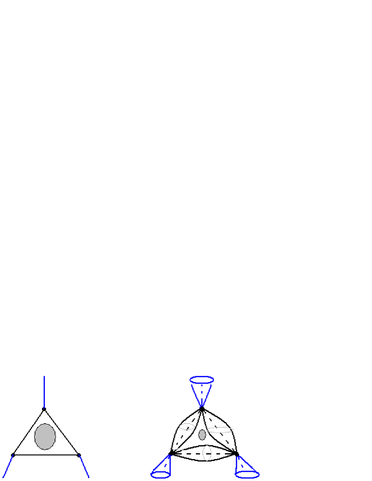
Figure 12: Toric graph of $\mathcal{O}\left(-3\right)\rightarrow$$E^{\left(t,\infty\right)}$. The compact part is $E^{\left(t,\infty\right)}$$=$$\left({\partial\mathbb{P}^{2}}\right)$ with the usual three vertices. Its toric frontier consists of three intersecting $\mathbb{P}^{1}$’s in the homology class of 2-torus . (a) Figure (on left) represents real skeleton. (b) Figure (on right) gives its fattening.

To get the superfield Lagrangian density $\mathcal{L}_{locT^{2}}$, we think about eqs(6.2) as the field equations of motion of the $D$ and $F_{i}$ auxiliary fields.
The first relation is associated with

$$\frac{\delta\mathcal{L}_{{\small locE}}}{\delta D}=0,$$ (6.3)

while the second follows from,

$$\frac{\delta\mathcal{L}_{{\small locE}}}{\delta F_{i}}=0.$$ (6.4)

The result is

$$\mathcal{L}_{{\small locE}} = \int d^{4}\theta\sum_{i=1}^{3}\overline{\Phi}_{i}e^{2V}\Phi_{i}+\int d^{4}\theta\left(\overline{\Phi}_{0}e^{-2mV}\Phi_{0}+\overline{\Phi}_{4}e^{2mV}\Phi_{4}\right)$$ (6.5)

$$+\mathcal{L}_{{\small gauge}}\left(V\right)-2t\int d^{4}\theta V+\left(g\int d^{2}\theta\Phi_{1}\Phi_{2}\Phi_{3}\Upsilon+hc\right),$$

where $\Upsilon$ is a Lagrange superfield multiplier capturing the constraint restricting the field variables to the boundary of $\mathbb{P}^{2}$.
In addition to the $U\left(1\right)$ gauge multiplet $V$, the chiral superfields of this model are

$$\left(\Phi_{0},\Phi_{1},\Phi_{2},\Phi_{4},\Phi_{5},\Upsilon\right)$$ (6.6)

and carry the following $q_{i}$- charges under the $U\left(1\right)$ gauge symmetry,

$$\left(q_{0},q_{1},q_{2},q_{3},q_{4},q_{\gamma}\right)=\left(-m,1,1,1,m,-3\right).$$ (6.7)

where $m$ is a priori equal to $3$; but in general can take any integral value.

6.2 Generalization

The construction we have developed here above can be generalized to other Calabi-Yau manifolds. Below we make a comment on two kinds of generalizations. The first extension deals with the gauged sigma model realization of local genus g-Riemann surfaces for $g\geq 2$. The second generalization concerns sigma model approach for higher complex dimensional compact toric Calabi-Yau manifolds.

6.2.1 Local genus g-Riemann surfaces

So far we have seen that for each local elliptic curve, it is associated a $U\left(1\right)$ gauge symmetry. This gauge symmetry is inherited from the $\mathbb{P}^{2}$ model. Since local genus g-Riemann surfaces can be engineered by gluing several local elliptic curves, we conclude that a class of local genus g-Riemann surfaces could be described by higher rank abelian $U^{n}\left(1\right)$ gauged supersymmetric field model type. The rank $n$ of the gauge symmetry depends on the way the gluing is done.
To illustrate the idea, let us give the example of $g=2$- Riemann surface described by a 2D $U^{2}\left(1\right)$ gauged $\mathcal{N}=2$ supersymmetric sigma model.
The local $g=2$- Riemann surface in the large complex structures limits can be engineered by gluing two local elliptic curves with compact base $E_{1}^{\left(t,\infty\right)}=\partial\mathbb{P}_{1}^{2}$ and $E_{2}^{\left(t,\infty\right)}=\partial\mathbb{P}_{2}^{2}$. In the sigma model approach, we distinguish different representations according to whether $\mathbb{P}_{1}^{2}$ and $\mathbb{P}_{2}^{2}$ have an intersection point or edge.
In the first case, the sigma model involves five complex field variables,

$$\left(z_{1},z_{2},z_{3},z_{4},z_{5}\right)$$ (6.8)

and a $U^{2}\left(1\right)$ gauge invariance under which these complex variables have the following gauge charges

$$\left(q_{i}^{1}\right) = \left(1,1,1,0,0\right)$$

$$\left(q_{i}^{2}\right) = \left(0,0,1,1,1\right)$$ (6.9)

The field theoretic equations describing the compact part of the moduli space of supersymmetric vacua are given by,

$$\left\{\begin{array}[]{c}\left|z_{1}\right|^{2}+\left|z_{2}\right|^{2}+\left|z_{3}\right|^{2}=t_{1}\\ z_{1}z_{2}z_{3}=0\end{array}\right.\qquad,\qquad\left\{\begin{array}[]{c}\left|z_{3}\right|^{2}+\left|z_{4}\right|^{2}+\left|z_{5}\right|^{2}=t_{2}\\ z_{3}z_{4}z_{5}=0\end{array}\right.,$$ (6.10)

where $t_{1}$ and $t_{2}$ are respectively the Kahler moduli of the projective planes $\mathbb{P}_{1}^{2}$ and $\mathbb{P}_{2}^{2}$. The holomorphic constraint eqs $z_{1}z_{2}z_{3}=0$ and $z_{3}z_{4}z_{5}=0$ are implemented in the gauged supersymmetric superfield model by two chiral superfields $\Upsilon_{1}$ and $\Upsilon_{2}$ with gauge charges $\left(q_{\gamma}^{1},q_{\gamma}^{2}\right)$ equal to $\left(-3,0\right)$ and $\left(0,-3\right)$ respectively.
Notice that eq(6.10) describes indeed a complex curve with genus $g=2$. The toric threefold based on this genus $g=2$ curve is parameterized by seven complex variables,

$$\left(z_{0},z_{1},z_{2},z_{3},z_{4},z_{5},z_{6}\right),$$ (6.11)

with gauge charges as

$$\left(q_{i}^{1}\right) = \left(-3,1,1,1,0,0,-3\right),$$

$$\left(q_{i}^{2}\right) = \left(-3,0,0,1,1,1,-3\right).$$ (6.12)

The gauged supersymmetric field theoretical equation

$$-m\left|z_{0}\right|^{2}+\left|z_{1}\right|^{2}+\left|z_{2}\right|^{2}+\left|z_{3}\right|^{2}+m\left|z_{6}\right|^{2} = t_{1},\qquad z_{1}z_{2}z_{3}=0,$$

$$-n\left|z_{0}\right|^{2}+\left|z_{3}\right|^{2}+\left|z_{4}\right|^{2}+\left|z_{5}\right|^{2}+n\left|z_{6}\right|^{2} = t_{2},\qquad z_{3}z_{4}z_{5}=0,$$ (6.13)

where $m$ and $n$ are in general arbitrary integers; but can be set equal to $3$ to keep in touch with the first Chern class of the complex two dimensional projective plane.
These relations involve seven complex variables constrained by four complex constraint eqs leaving then three complex variables free. Note also that the first relation of the above equation describes $\mathcal{O}\left(m\right)\oplus\mathcal{O}\left(-m\right)\rightarrow E_{1}^{\left(t,\infty\right)}$ while the second describes $\mathcal{O}\left(n\right)\oplus\mathcal{O}\left(-n\right)\rightarrow E_{2}^{\left(t,\infty\right)}$.

6.2.2 Higher dimensional toric CY manifolds

The gauged supersymmetric sigma model for the boundary surface of local $\mathbb{P}^{2}$ that we have considered in this paper can be extended for compact divisors of local $\mathbb{P}^{n-1}$. The latter is given by the following $U\left(1\right)$ gauge invariant complex dimension $n$ hypersurface

$$n\left|z_{0}\right|^{2}+\sum_{i=1}^{n}\left|z_{i}\right|^{2}=t,$$ (6.14)

embedded in $\mathbb{C}^{n+1}$ parameterized by the local coordinates $\left\{z_{0},z_{1},z_{2},...,z_{n}\right\}$ with gauge charge

$$\left(q_{0},q_{1},q_{2},...,q_{n}\right)=\left(-n,1,1,...,1\right)$$ (6.15)

In eq(6.14), $t$ is the usual Kahler parameter of $\mathbb{P}^{n-1}$. To describe the compact (divisor) boundary $\partial\left(\mathbb{P}^{n-1}\right)$ of the toric n-fold, we supplement the hypersurface equation by the following extra gauge covariant constraint relation,

$$\mathop{\displaystyle\prod}\limits_{i=1}^{n}z_{i}=0.$$ (6.16)

Extending the analysis of section 4, the $U\left(1\right)$ gauged supersymmetric sigma model describing $\partial\left(\mathbb{P}^{n-1}\right)$ reads as follows

$$\mathcal{L}_{\partial P^{n-1}}=\mathcal{L}_{P^{n-1}}+\left(g\int d^{2}\theta W\left(\Phi,\Upsilon\right)+hc\right)$$ (6.17)

with chiral superpotential

$$W\left(\Phi,\Upsilon\right)=\Upsilon\mathop{\displaystyle\prod}\limits_{i=1}^{n}\Phi_{i}.$$ (6.18)

The gauge charge $q_{\gamma}$ of the Lagrange multiplier superfield $\Upsilon$ is equal to $\left(-n\right)$. Here also the first Chern class of $\partial\left(\mathbb{P}^{n-1}\right)$ is identically zero. As noted before, this property is not a new feature since the most general gauge invariant chiral superpotential extending eq(6.18) is given by

$$W\left(\Phi,\Upsilon\right)=\sum_{m_{1}+...+m_{n}=n}g_{\left\{m_{i}\right\}}\left(\Upsilon\mathop{\displaystyle\prod}\limits_{i=1}^{n}\Phi_{i}^{m_{i}}\right)$$ (6.19)

where $g_{\left\{m_{i}\right\}}$ are complex coupling constants.
The equation of motion of $\Upsilon$ gives a degree $n$ homogeneous polynom describing a complex $\left(n-2\right)$ dimension holomorphic CY hypersurface with complex structures $g_{\left\{m_{i}\right\}}$.

7 Conclusion

In this paper, we have set up the basis of the non planar topological 3-vertex method to compute the topological string amplitudes for the family of local elliptic curves

$$\mathcal{O}(m)\oplus\mathcal{O}(-m)$$ , ,

(7.1)

in the limit of large complex structure $\mathrm{\mu}$; i.e

$$\left|\mathrm{\mu}\right|$$ .

(7.2)

Generally speaking, the base $E^{\left(t,\mathrm{\mu}\right)}$ stands for an elliptic curve with Kahler parameter $t$ and complex structure $\mathrm{\mu}$ embedded in the projective plane $\mathbb{P}^{2}$. In the large limit $\mathrm{\mu}$; the corresponding elliptic curve $E^{\left(t,\mathrm{\infty}\right)}$ is realized as the toric boundary of $\mathbb{P}^{2}$; see appendix for more details; in particular eqs(8.5,8.12,8.17).
First, we have reviewed the main idea of the usual (planar) topological 3-vertex method for non compact toric threefolds.
Then, we have drawn the first lines of the non planar topological 3-vertex method for the local degenerate 2-torus. The latter is a non compact toric Calabi-Yau threefold given by a hypersurface in a complex Kahler 4-fold.
The key idea in getting the particular toric representation of the local 2-torus with large complex structure is based on thinking about $E^{\left(t,\infty\right)}$ as given by the toric boundary of the complex projective plane $\mathbb{P}^{2}$. In this view, $\mathcal{O}(m)\oplus\mathcal{O}(-m)\rightarrow E^{\left(t,\infty\right)}$ becomes a toric threefold and so one may extend the results of the topological 3- vertex method of [28] to the case of the local (degenerate) 2-torus. Obviously, to compute the topological amplitudes, we have to use the non planar 3-vertex method rather than the usual planar 3-vertex one. Regarding this matter, we have given first results concerning the local degenerate elliptic curve $\mathcal{O}(m)\oplus\mathcal{O}(-m)\rightarrow E^{\left(t,\infty\right)}$. More analysis is however still needed before getting the complete explicit results.

We have also developed the gauged supersymmetric sigma model realization that underlies the geometry the local 2-torus with $\left|\mathrm{\mu}\right|\longrightarrow\infty$ and exhibited explicitly the role of D- and F- terms. We have discussed as well how this construction could be extended to local genus g-Riemann surfaces $\mathcal{O}(m)\oplus\mathcal{O}(2-2g-m)$ $\rightarrow\Sigma_{g}$ in the limit of large complex structures.
The results obtained in the field theory part of the paper may also be viewed as an explicit analysis regarding implementation of F- terms in the Witten’s original work on phases of $\mathcal{N}=2$ supersymmetric theories in two dimensions [47].

Acknowledgement 1

The authors thank the International Centre for Theoretical Physics, and S. Randjabar Daemi for kind hospitality at ICTP. This research work is supported by Protars III CNRST-D12/25.

8 Appendix

In this appendix, we give useful properties on the complex projective plane and on particular aspects on the complex curves in $\mathbb{P}^{2}$.
More precisely denoting by $\mathbb{P}_{t}^{2}$, the projective plane with Kahler parameter $t$ and by $E^{\left(t,\mu\right)}$ the following elliptic curve in $\mathbb{P}_{t}^{2}$,

$$E^{\left(t,\mu\right)}:\qquad z_{1}^{3}+z_{2}^{3}+z_{3}^{3}+\mu z_{1}z_{2}z_{3}=0$$

we want to show that the boundary $\partial\left(\mathbb{P}_{t}^{2}\right)$ is nothing but the degenerate limit $\mathrm{\mu\longrightarrow\infty}$ of $E^{\left(t,\mu\right)}$; that is

$$\partial\left(\mathbb{P}_{t}^{2}\right)\simeq E^{\left(t,\infty\right)}.$$ (8.1)

This question can be also rephrased in other words by using the fibration,

$$\mathbb{P}^{2}=\mathcal{B}_{2}\times\mathbb{T}^{2},$$ (8.2)

where $\mathcal{B}_{2}$ is real 2 dimensional base (an equilateral triangle). The boundary $\partial\left(\mathbb{P}^{2}\right)$ is a toric submanifold with fibration

$$\partial\left(\mathbb{P}^{2}\right)$$ ,

(8.3)

where $\Delta_{1}=\left(\partial\mathcal{B}_{2}\right)$ is the boundary of a triangle.
Clearly, thought not exactly the standard 2- torus $\mathbb{S}^{1}\times\mathbb{S}^{1}$, the boundary $\partial\left(\mathbb{P}^{2}\right)$ has something to do with it. It is the large complex structure $\mu$ of the elliptic curve $E^{\left(t,\mu\right)}$; say

$$\left|\mu\right|$$ .

(8.4)

As we need both Kahler and complex structures to answer the question (8.1), let us first give some useful details and then turn to derive the identity $\partial\left(\mathbb{P}_{t}^{2}\right)\simeq E^{\left(t,\infty\right)}$.

Projective plane $\mathbb{P}^{2}$
There are different ways to deal the complex projective plane $\mathbb{P}^{2}$. Below, we give two dual descriptions by using the so called type IIA and type IIB geometries [51].

Type IIA geometry
In this set up, known also as toric geometry, the projective plane $\mathbb{P}^{2}$ is defined by the following real 4 dimensional compact hypersurface in $\mathbb{C}^{3}$,

$$\left|z_{1}\right|^{2}+\left|z_{2}\right|^{2}+\left|z_{3}\right|^{2}=t,$$ (8.5)

where $\left(z_{1},z_{2},z_{3}\right)$ stand for local complex coordinates. In the above relation, the complex variables obey the gauge identifications

$$z_{k}^{\prime}$$ ,

(8.6)

where the real phase $\varphi$ is the parameter of the $U\left(1\right)$ gauge symmetry. The phase $\varphi$ can be used to fix one of the three phases of the $z_{k}=\left|z_{k}\right|e^{i\varphi_{k}}$ complex coordinates leaving then two free phases; say $\varphi_{1}$ and $\varphi_{2}$. These free phases are precisely the ones used to parameterize the 2-torus in the fibration (8.2).
The positive parameter $t$ is the Kahler modulus of the projective plane; it controls the size of $\mathbb{P}^{2}$. Indeed, in the singular limit $t\longrightarrow 0$, we have the two following:
(i) the size of the complex surface $\mathbb{P}^{2}$ vanishes

$$\lim_{t\longrightarrow 0}\left[vol\left(\mathbb{P}^{2}\right)\right]=0,$$ (8.7)

in agreement with both the relation $vol\left(\mathbb{P}^{2}\right)\sim t^{2}$ (footnote 7) and eq(8.5) which becomes then singular.
(ii) the size of the complex boundary $\partial\left(\mathbb{P}^{2}\right)$ vanishes as well

$$\lim_{t\longrightarrow 0}\left[vol\left[\partial\left(\mathbb{P}^{2}\right)\right]\right]=0,$$ (8.8)

The two above relations show that the Kahler parameter $t$ of $\mathbb{P}^{2}$ and the Kahler parameter $r$ of it boundary $\partial\left(\mathbb{P}^{2}\right)$ are intimately related. We will show later that they are the same.
Notice in passing that in the field theory language, the relation (8.5) has an interpretation as the field equation of motion of the D- auxiliary field in the $U\left(1\right)$ gauged sigma model realization of $\mathbb{P}^{2}$. There, the Kahler parameter $t$ is interpreted as the Fayet-Iliopoulos coupling constant term. This description is well known; some of its basic aspects have been studied in section 4 of this the paper; we will then omit redundant details.

Type IIB geometry:
In the type IIB geometry, one thinks about the complex projective surface $\mathbb{P}^{2}$ as a complex holomorphic algebraic surface obtained by taking the coset of the complex space $\mathbb{C}^{3}\backslash\left\{\left(0,0,0\right)\right\}$ by the complex abelian group $\mathbb{C}^{\ast}$;

$$\mathbb{P}^{2}=\left[\mathbb{C}^{3}\backslash\left\{\left(0,0,0\right)\right\}\right]/\mathbb{C}^{\ast}.$$ (8.9)

The $\mathbb{C}^{\ast}$ group action allows to make the following identifications,

$$\left(z_{1},z_{2},z_{3}\right)\equiv\left(\lambda z_{1},\lambda z_{2},\lambda z_{3}\right)$$ (8.10)

with $\lambda$ being an arbitrary non zero complex number. This identification reduces the complex 3- dimension down to complex 2 dimensions. Here also, one can make gauge choices by working in a particular local coordinate patch. A standard gauge choice is the one given by the condition $\lambda z_{3}=1$.

Complex curves in $\mathbb{P}^{2}$
Complex curves ( real Riemann surfaces) in $\mathbb{P}^{2}$ are complex codimension one submanifolds obtained by imposing one more complex constraint relation $\mathrm{f}\left(z_{i}\right)=0$ on the projective complex variables $z_{1},z_{2}$ and $z_{3}$. The most common curves in $\mathbb{P}^{2}$ are obviously the projective lines $\mathbb{P}^{1}$, conics and elliptic curves.
Generally speaking, the constraint eq $\mathrm{f}\left(z_{i}\right)=0$ can be stated as follows,

$$\mathrm{f}\left(\lambda z_{1},\lambda z_{2},\lambda z_{3}\right)=\lambda^{n}\mathrm{f}\left(z_{1},z_{2},z_{3}\right)=0,$$ (8.11)

where $n$ stands for the degree of homogeneity of the curve. The case $n=3$, is given by the following typical cubic

$$z_{1}^{3}+z_{2}^{3}+z_{3}^{3}+\mu z_{1}z_{2}z_{3}=0.$$ (8.12)

This relation describes an elliptic curve $E$ of degree 3 with a complex structure $\mu$. This curve $E$ has been extensively used in physical literature; in particular in the geometric engineering of 4D superconformal field theories embedded in 10D type IIB superstring on elliptically fibered Calabi-Yau threefolds [51, 52].
Before proceeding further, it is interesting to notice that the elliptic curve $E$ is a genus one Riemann surface having a real 3d moduli space; parameterized by

$$\left(\mu_{1},\mu_{2};r\right)$$ (8.13)

with $\mu=\mu_{1}+i\mu_{2}$ is the complex structure and $r$ is its Kahler modulus. So, elliptic curves may be generally denoted as follows

$$E^{\left(r,\mu\right)}.$$ (8.14)

Regarding the complex parameter $\mu$ of the elliptic curve $E^{\left(r,\mu\right)}$, it is explicitly exhibited in type IIB geometry set up as shown on eq(8.12).
However, it is interesting to notice that the Kahler parameter $r$ cannot be exhibited explicitly since $E^{\left(r,\mu\right)}$ has no standard type IIA geometry realisation of the type given by eq(8.5).
The construction developed in this paper gives a way to circumvent this difficulty by using the degenerate representation (8.3).
With the above features in mind, we turn now to the derivation of eq(8.1).

$\partial\left(\mathbb{P}^{2}\right)$ as the degenerate elliptic curve $E^{\left(r,\infty\right)}$ 
Here we would like to show that $\partial\left(\mathbb{P}^{2}\right)$ is $E^{\left(r,\mu\right)}$ but with a large complex structure $\mu$; that is $\left|\mu\right|\longrightarrow\infty$.
To get the key point behind the identity (8.1) as well as the degeneracy of the elliptic curve $E^{\left(r,\mu\right)}$, we give the two following properties:
(a) the projective plane $\mathbb{P}^{2}$ has three particular intersecting divisors $\mathcal{D}_{i}$. These are associated with the hyperlines

$$z_{i}=0$$ (8.15)

in $\mathbb{P}^{2}$ which, up on using eq(8.5), lead to the following relations

$$\mathcal{D}_{1}$$ ,

,

.

(8.16)

From these equations, we see that each divisor $\mathcal{D}_{i}$ is a projective line with Kahler parameter $t$.
The equality of the Kahler parameters $t_{1}=t_{2}=t_{3}=t$ of these projective lines may be also interpreted as due to the permutation symmetry of the $\left\{z_{i}\right\}$ projective coordinate variables of $\mathbb{P}^{2}$. This feature translates, in the language of toric geometry, as corresponding to having an equilateral triangle for the real base $\mathcal{B}_{2}$.
(b) The divisors $\left\{\mathcal{D}_{i}\right\}$ are precisely the ones we get by taking the large complex structure limit (8.4) of the complex curve eq(8.12). Under this condition, eq(8.12) reduces then to the dominant monomial

$$\mu z_{1}z_{2}z_{3}=0.$$ (8.17)

Notice that the above relation is obviously invariant under the $\mathbb{C}^{\ast}$ transformations (8.10) since

$$\mu\left(\lambda z_{1}\right)\left(\lambda z_{2}\right)\left(\lambda z_{3}\right)=\lambda^{3}\left(\mu z_{1}z_{2}z_{3}\right)=0.$$ (8.18)

To have more insight about the elliptic curve $E^{\left(t,\infty\right)}$ with large complex structure; $\left|\mu\right|\longrightarrow\infty$, it is interesting to solve eq(8.17). There are three solutions classified as follows:
(i) $z_{1}=0$, what ever the two other complex variables $z_{2}$ and $z_{3}$ are; provided that

$$\left(z_{2},z_{3}\right)$$ ,

.

(8.19)

But these relations are nothing but the definition of the divisor $\mathcal{D}_{1}$ in type IIB geometry.
(ii) $z_{2}=0$, what ever the other complex variables $z_{1}$ and $z_{3}$ are; provided that

$$\left(z_{1},z_{3}\right)$$ ,

,

(8.20)

describing then the divisor $\mathcal{D}_{2}$.
(iii) $z_{3}=0$, what ever the other complex variables $z_{2}$ and $z_{1}$ are; provided that

$$\left(z_{1},z_{2}\right)$$ ,

,

(8.21)

associated with the divisor $\mathcal{D}_{3}$.
To conclude the boundary $\left(\partial\mathbb{P}_{t}^{2}\right)$ of the projective plane $\mathbb{P}_{t}^{2}$ is indeed described by an elliptic curve with a Kahler parameter $t$ inherited from the $\mathbb{P}_{t}^{2}$ one; but with a large complex structure $\mu$; see also footnote 7. The limit $\mu\rightarrow\infty$ explains the degeneracy property in the base $\Delta_{1}$ (8.3).

References

- [1] Marcos Marino, Chern-Simons Theory and Topological Strings, Rev.Mod.Phys. 77 (2005) 675-720, arXiv:hep-th/0406005
- [2] R. Dijkgraaf, E. Verlinde, H. Verlinde, “Notes on topological string theory and two-dimensional topological gravity,” in String theory and quantum gravity, World Scientific Publishing, p. 91, (1991)
- [3] M. Bershadsky, S. Cecotti, H. Ooguri and C. Vafa, “Kodaira-Spencer theory of gravity and exact results for quantum string amplitudes,” Commun. Math. Phys. 165, 311 (1994), hep-th/9309140.
- [4] G. L. Cardoso, B. de Wit, J. Kappeli, T. Mohaupt, Stationary BPS Solutions in N=2 Supergravity with R-Interactions, JHEP 0012 (2000), 019arXiv:hep-th/0009234,
- [5] A. Ceresole, R. D’Auria, S. Ferrara, The Symplectic Structure of N=2 Supergravity and its Central Extension, Nucl.Phys.Proc.Suppl. 46 (1996) 67-74, arXiv:hep-th/9509160,
- [6] T. Graber and E. Zaslow, “Open string Gromov-Witten invariants: Calculations and a mirror ’theorem’” arXiv:hep-th/0109075.
- [7] M. Aganagic, A. Klemm, and C. Vafa, “Disk Instantons, Mirror Symmetry and the Duality Web,” hep-th/0105045.
- [8] J.Bryan, R.Pandharipande, Curves in Calabi-Yau and topological quantum field theory, Duke Math.126 (2005) 369-396. J.Bryan, R.Pandharipande, On the rigidity of stable maps to Calabi-Yau threefolds, Geometry Topology Monographs 8 (2006) 97-104
- [9] Jim Bryan and Rahul Pandharipande, The local Gromov-Witten theory of curves, math.AG/0411037 v3 2006
- [10] D.Karp, C.Liu, M.Marino, The local Gromov-Witten invariants of configuration of rational curves, Geometry Topology Monographs 10 (2006) 115-168
- [11] H. Ooguri, A. Strominger, C. Vafa, Black Hole Attractors and the Topological String, Phys. Rev. D70 (2004) 106007, hep-th/0405146.
- [12] C. Vafa, Two dimensional Yang-Mills, black holes and topological strings,hep-th/0406058.
- [13] A. Dabholkar, Exact counting of black hole microstates, Phys. Rev. Lett. 94 (2005) 241-301, hep-th/0409148.
- [14] H. Ooguri, C. Vafa, E. Verlinde, Hartle-Hawking Wave-Function for Flux Compactifications, Lett. Math. Phys. 74 (2005) 311-342, hep-th/0502211.
- [15] R. Dijkgraaf, R. Gopakumar, H. Ooguri, C. Vafa, Baby Universes in String Theory, Phys. Rev. D73 (2006) 066002, hep-th/0504221.
- [16] A. Belhaj, L. B. Drissi, E. H. Saidi, A. Segui, Supersymmetric Black Attractors in Six and Seven Dimensions, arXiv:0709.0398, Nuclear Physics B 796 [FS] (2008) 521–580.
- [17] El Hassan Saidi, Moulay Brahim Sedra, Topological string in harmonic space and correlation functions in S^3 stringy cosmology.Nucl.Phys.B748:380-457,2006, hep-th/0604204
- [18] M. Aganagic, A. Neitzke, C. Vafa, BPS Microstates and the Open Topological String Wave Function, hep-th/0504054
- [19] E. Witten, “Topological Sigma Models,” Commun. Math. Phys. 118, 411 (1988).
- [20] M. Bershadsky, S. Cecotti, H. Ooguri, and C. Vafa, “Holomorphic Anomalies in Topological Field Theories,” Nucl. Phys. 405B (1993) 279-304;
- [21] H. Ooguri and C. Vafa, “Knot invariants and topological strings,” Nucl. Phys. B 577,419 (2000), [arXiv:hep-th/9912123].
- [22] J. Walcher, “Extended Holomorphic Anomaly and Loop Amplitudes in Open Topological, String,” arXiv[hep-th]:0705.4098 .
- [23] S. Yamaguchi and S. T. Yau, “Topological string partition functions as polynomials,” JHEP 0407, 047 (2004) [arXiv:hep-th/0406078].
- [24] M. Alim and J. D. Lange, “Polynomial Structure of the (Open) Topological String Partition Function,” JHEP 0710, 045 (2007) arXiv [hep-th]:0708.2886.
- [25] M. Aganagic, R. Dijkgraaf, A. Klemm, M. Marino and C. Vafa, “Topological strings and integrable hierarchies,” Commun. Math. Phys. 261, 451 (2006), [arXiv:hep-th/0312085].
- [26] V. Bouchard, B. Florea and M. Marino, “Topological open string amplitudes on orientifolds,” JHEP 0502, 002 (2005) [arXiv:hep-th/0411227].
- [27] M. Aganagic and C. Vafa, “Mirror Symmetry, D-Branes and Counting Holomorphic Discs,” arXiv:hep-th/0012041.
- [28] M. Aganagic, A. Klemm, M. Marino, C. Vafa, The Topological Vertex, Commun. Math. Phys. 254 (2005) 425-478, hep-th/0305132.
- [29] A. Iqbal, A-K Kashani-Poor, The Vertex on a Strip, hep-th/0410174, Instanton Counting and Chern-Simons Theory, Adv. Theor. Math. Phys. 7 (2004) 457-497, hep-th/0212279.
- [30] Amer Iqbal, Can Kozcaz, Cumrun Vafa, The Refined Topological Vertex, arXiv:hep-th/0701156,
- [31] Piotr Sulkowski, Crystal Model for the Closed Topological Vertex Geometry, JHEP 0612 (2006) 030, arXiv:hep-th/0606055,
- [32] A. Iqbal, C. Kozcaz and C. Vafa, “The refined topological vertex,” arXiv:hep-th/0701156.
- [33] Masato Taki, Refined Topological Vertex and Instanton Counting , arXiv::hep-th/0710.1776
- [34] N. A. Nekrasov, “Seiberg-Witten prepotential from instanton counting,” Adv. Theor. Math. Phys. 7, 831 (2004) [arXiv:hep-th/0206161]
- [35] N. Nekrasov and A. Okounkov, “Seiberg-Witten theory and random partitions,” arXiv:hepth/0306238.
- [36] H. Nakajima and K. Yoshioka, “Instanton counting on blowup. I. 4-dimensional pure gauge theory,” Invent. Math 162, no. 2, 313 (2005) [arXiv:math.A.G/0306198].
- [37] A. Braverman and P. Etingof, “Instanton counting via affine Lie algebras II: from Whittaker vectors to the Seiberg-Witten prepotential” arXiv:math.AG/0409441.
- [38] A. Iqbal and A. K. Kashani-Poor, “Instanton counting and Chern-Simons theory,” Adv. Theor.Math. Phys. 7, 457 (2004) [arXiv:hep-th/0212279]. “SU(N) geometries and topological string amplitudes,” Adv. Theor. Math. Phys. 10, 1 (2006) [arXiv:hep-th/0306032].
- [39] T. Eguchi and H. Kanno, “Topological strings and Nekrasov’s formulas,” JHEP 0312, 006 (2003) [arXiv:hep-th/0310235].
- [40] T. J. Hollowood, A. Iqbal and C. Vafa, “Matrix Models, Geometric Engineering and Elliptic Genera,” arXiv:hep-th/0310272.
- [41] C. Vafa, “Two dimensional Yang-Mills, black holes and topological strings,” hepth/0406058.
- [42] N. Caporaso, M. Cirafici, L. Griguolo, S. Pasquetti, D. Seminara, R. J. Szabo, Topological Strings, Two-Dimensional Yang-Mills Theory and Chern-Simons Theory on Torus Bundles, hep-th/0609129.
- [43] R. Ahl Laamara, A. Belhaj, L.B. Drissi, E.H. Saidi, Black Holes in Type IIA String on Calabi-Yau Threefolds with Affine ADE Geometries and q-Deformed 2d Quiver Gauge Theories, arXiv:hep-th/0611289, Nucl.Phys.B776:287-326,2007
- [44] S. Katz, P. Mayr, C. Vafa, Mirror symmetry and Exact Solution of 4D N=2 Gauge Theories I, Adv. Theor. Math. Phys. 1 (1998) 53-114, hep-th/9706110.
- [45] M. Ait Ben Haddou, A. Belhaj, E.H. Saidi, Geometric Engineering of N=2 CFT4s based on Indefinite Singularities: Hyperbolic Case, Nucl. Phys. B674 (2003) 593-614, hep-th/0307244.
- [46] R. Ahl Laamara, M. Ait Ben Haddou, A. Belhaj, L.B. Drissi, E.H. Saidi, RG Cascades in Hyperbolic Quiver Gauge Theories, Nucl. Phys. B702 (2004) 163-188, hep-th/0405222.
- [47] Edward Witten, Phases of N=2 Theories In Two Dimensions, Nucl.Phys. B403 (1993) 159-222, arXiv:hep-th/9301042
- [48] N.C. Leung, C. Vafa, Branes and Toric Geometry, Adv. Theor. Math.Phys. 2 (1998) 91-118, hep-th/9711013.
-
[49]
L.B. Drissi, H. Jehjouh, E.H. Saidi, Topological String
on Local Elliptic Curve
with Large Complex Structure, Afr Journal Of Mathematical Physics, Volume 6 (2007) 83-91. - [50] Lalla Btissam Drissi, Houda Jehjouh, El Hassan Saidi, Generalized MacMahon G(q) as q-deformed CFT Correlation Function, arXiv:0801.2661, To appear in Nucl Phys B (2008),
- [51] S. Katz, P. Mayr, C. Vafa, Mirror symmetry and Exact Solution of 4D N=2 Gauge Theories I, Adv.Theor.Math.Phys. 1 (1998) 53-114, arXiv:hep-th/9706110
- [52] A. Belhaj, A. Elfallah, E.H. Saidi, On the non-simply laced mirror geometries in type II strings, Class.Quant.Grav.17:515-532,2000, On the Affine D(4) mirror geometry, Class.Quant.Grav.16:3297-3306,1999