Drift reversal in asymmetric coevolutionary conflicts:
Influence of microscopic processes and population size

Abstract

The coevolutionary dynamics in finite populations currently is investigated in a wide range of disciplines, as chemical catalysis, biological evolution, social and economic systems. The dynamics of those systems can be formulated within the unifying framework of evolutionary game theory. However it is not a priori clear which mathematical description is appropriate when populations are not infinitely large. Whereas the replicator equation approach describes the infinite population size limit by deterministic differential equations, in finite populations the dynamics is inherently stochastic which can lead to new effects. Recently, an explicit mean-field description in the form of a Fokker-Planck equation was derived for frequency-dependent selection in finite populations based on microscopic processes. In asymmetric conflicts between two populations with a cyclic dominance, a finite-size dependent drift reversal was demonstrated, depending on the underlying microscopic process of the evolutionary update. Cyclic dynamics appears widely in biological coevolution, be it within a homogeneous population, or be it between disjunct populations as female and male. Here explicit analytic address is given and the average drift is calculated for the frequency-dependent Moran process and for different pairwise comparison processes. It is explicitely shown that the drift reversal cannot occur if the process relies on payoff differences between pairs of individuals. Further, also a linear comparison with the average payoff does not lead to a drift towards the internal fixed point. Hence the nonlinear comparison function of the frequency-dependent Moran process, together with its usage of nonlocal information via the average payoff, is the essential part of the mechanism.

Introduction

Biology offers a rich laboratory of various types of oscillatory, chaotic and stochastic dynamics. Recently cyclic evolutionary dynamics has been observed in E.coli in vitro kerr and in vivo kirkup , and attracted interest as a possible mechanism to stabilize biodiversity. This contributes to a long-standing debate how the emergence of new mutants is maintained in biological evolution: Cyclic dynamics has been one of the first proposals for such mechanisms hypercycle . Cyclic coevolution is not only observed in asexual reproduction. A prominent observation of cyclic domination is observed in side-blotched lizards lizards ; Zam00 . Three territorial mating behaviour strategies of the male lizards occur, and coincide genetically with orange, blue and yellow blotches. While the cyclic dynamics of rock-paper-scissors type can be demonstrated without taking males and females into account explicitely, hereby an improved quantitative understanding is possible Sinervo01 .

Social and economic systems are a likewise interesting class of systems in which cyclic dynamics is observed. Social individua deciding in economic situations helbing92physicaa ; helbing92physicaa193 ; helbing93physicaa196 ; helbing05pre ; helbing94socialfield ; helbing94pair ; helbing96decision can fall into oscillatory cycles, e.g. when loners, not participating in the game, are added as a third strategy to a Prisoner’s Dilemma loners ; szabohauert02 . Evolutionary game theory is a unifying approach for such systems nowak06book ; szaboreview ; miekiszreview .

In this paper, a paradigmatic cyclic game is analyzed, which is of likewise importance, for biological mating behaviour, as well as in human social decision dynamics: Dawkins’ “Battle of the Sexes” (BOTS), a 2$\times$2 bimatrix game, is the simplest possible type of a cyclic game played by individuals between two homogeneous, mixed populations dawkins . In the mating behaviour of females and males, a cyclical dominance of ‘slow’ and ‘fast’ strategies can lead to a “Battle of the Sexes”, or oscillations, in the infinite population replicator dynamics dawkins ; hofbauer98 ; magurran . The inherent stochasticity in a finite population moran ; nowak04 ; taylor04 refines this picture, depending on population size and underlying process TCH05 ; CT05 ; TCH06 ; reichenbach06 ; CT06 ; C08 .

The aim of the paper is to investigate in detail the drift reversal firstly reported in TCH05 , and to corrobate the simulations with an analytic result, allowing for a refined insight into the drift reversal. The main results are (i) that for a generic class of pairwise comparison processes a drift reversal does not occur, and (ii) that for the Moran process, the combination of both a nonlinear reproductive fitness and the comparison with a global function (average fitness) are necessary for a drift reversal.

The paper is organized as follows. In Section 1, the BOTS payoff matrices are introduced and the infinite population description of evolutionary game theory by the replicator equation is recalled. In Section 2, evolutionary birth-death processes are defined in a unifying framework for comparison. In Section 3 the influence of the stochasticity on the time evolution of the population densities is motivated by computer simulations of the process.

In the main Section 4, the average drift (more formally introduced in Sect. 4.1) of the BOTS dynamics is calculated explicitely in finite populations, and the population size corrections are obtained to first and second order analytically for four microscopic interaction processes, for neutral evolution as well as for two linear processes, the Local Update and the linearized Moran process. The paper concludes by discussing and summarizing the results.

1 Battle of the Sexes: Replicator dynamics

This is the simplest cyclic game between two populations. Following Dawkins dawkins , the elementary payoffs read

$$\left(\begin{array}[]{c}\pi_{A}^{\text{\Female}}\\ \pi_{B}^{\text{\Female}}\end{array}\right)=\left(\begin{array}[]{cc}-1&+1\\ +1&-1\end{array}\right)\left(\begin{array}[]{c}x\\ 1-x\end{array}\right)$$ (7)

$$\left(\begin{array}[]{c}\pi_{A}^{\text{\Male}}\\ \pi_{B}^{\text{\Male}}\end{array}\right)=\left(\begin{array}[]{cc}+1&-1\\ -1&+1\end{array}\right)\left(\begin{array}[]{c}y\\ 1-y\end{array}\right)$$ (14)

for agents interacting with a population of $(x,y,1-x,1-y)$ $=(i/N,j/N,(N-i)/N,(N-j)/N)$ agents in the strategies $(\pi_{A}^{\text{\Male}},\pi_{A}^{\text{\Female}},\pi_{B}^{\text{\Male}},\pi_{B}^{\text{\Female}})$. As the opponent’s payoff matrix is not the simple transpose of the proponent’s payoff matrix, such games are called bimatrix games or asymmetric conflicts. While in the replicator equations hofbauer98 picture the population cannot go extinct due do lack of discreteness, for the stochastic description in this paper the population size will be fixed to $N$ female and $N$ male individuals.

For the relative frequencies, or abundance densities, evolutionary game theory, with the implicit assumption of an infinite population, considers the replicator equation

$$\dot{x} = x(\pi^{A}_{\text{\Male}}-\langle\pi_{\text{\Male}}\rangle)$$ (15)

$$\dot{y} = y(\pi^{A}_{\text{\Female}}-\langle\pi_{\text{\Female}}\rangle)$$ (16)

For the standard parameter choice (equivalent to “Matching Pennies”) of the BOTS the replicator equation has a constant of motion

$$H=-x(1-x)y(1-y).$$ (17)

The replicator equations exhibits neutrally stable oscillations around the $x=y=1/2$ fixed point; the adjusted replicator equation (see hofbauer98 ) has an attractive stable fixed point. In so-called asymmetric conflicts (bimatrix games) where members of the two (sub)populations can receive different payoffs, both populations may gain different average payoffs, and the denominators in the adjusted replicator equations (being the proper $N\to\infty$ limit of the Moran process, see TCH06 )

$$\dot{x} = \frac{x(\pi^{A}_{\text{\Male}}-\langle\pi_{\text{\Male}}\rangle)}{\frac{1-w}{w}+\langle\pi_{\text{\Male}}\rangle}$$ (18)

$$\dot{y} = \frac{y(\pi^{A}_{\text{\Female}}-\langle\pi_{\text{\Female}}\rangle)}{\frac{1-w}{w}+\langle\pi_{\text{\Female}}\rangle}$$ (19)

are different, as $\langle\pi_{\text{\Male}}\rangle=-\langle\pi_{\text{\Female}}\rangle$. Thus the denominators cannot be absorbed into a dynamical rescale of time (velocity transformation) and both types of replicator equations not necessarily exhibit the same stability properties.

How is this behaviour changed, and how far is it preserved in finite populations? This is the central question addressed in this paper.

2 Evolutionary processes

To study dynamics in finite populations, it is advised to go down to the microscopic interactions, and to derive macroscopic equations of motion herefrom, eventually utilizing a finite-size expansion to derive fluctuation corrections to the deterministic limit. As the microscopic dynamics may depend on the system at hand, the respective biological or behavioral setup may require different interaction and competition processes. These, however, can be cast into a unifying framework. Following previous investigations helbing92physicaa ; TCH05 , we consider two classes of birth-death processes: the frequency-dependent Moran process moran ; nowak04 ; taylor04 describing competition with the whole population, and local two-particle interaction processes, with linear TCH05 or Fermi-type szabohauert02 ; blume ; TNP06 dependence of the reproductive fitness as a function of the payoff difference between two competing agents. For all processes, the payoffs for an individual read

$$\pi_{A}^{\text{\Male}} = 2y-1\mbox{~{}~{}~{}~{}~{}~{}}\pi_{A}^{\text{\Female}}=1-2x$$

$$\pi_{B}^{\text{\Male}} = 1-2y\mbox{~{}~{}~{}~{}~{}~{}}\pi_{B}^{\text{\Female}}=2x-1.$$ (20)

2.1 Moran process

The Moran process moran , a birth-death process, thus preserving $N$, is a standard model of mathematical genetics describing random inheritance in overlapping generations. In its original formulation, fitnesses of the genetic types were independent of abundance densities in the population, i.e., coevolution was not taken into account. In the frequency-dependent Moran process nowak04 ; taylor04 , each individual competes with the whole population, or an representative fraction of it, and reproduces proportional to this (cumulative) payoff normalized by the average payoff in the population. With the payoffs averaged over the respective population,

$$\langle\pi^{\text{\Male}}\rangle = \frac{i}{N}\pi_{A}^{\text{\Male}}+\frac{N-i}{N}\pi_{B}^{\text{\Male}}$$ (21)

$$\langle\pi^{\text{\Female}}\rangle = \frac{j}{N}\pi_{A}^{\text{\Female}}+\frac{N-j}{N}\pi_{B}^{\text{\Female}}$$ (22)

for given $(i,j)$ the transition probabilities of the possible four hopping events are given by

$$T^{+\bullet} = \frac{1}{2}\frac{1-w+w\pi_{A}^{\text{\Male}}}{1-w+w\langle\pi^{\text{\Male}}\rangle}\frac{i}{N}\frac{N-i}{N}$$

$$T^{-\bullet} = \frac{1}{2}\frac{1-w+w\pi_{B}^{\text{\Male}}}{1-w+w\langle\pi^{\text{\Male}}\rangle}\frac{i}{N}\frac{N-i}{N}$$

$$T^{\bullet+} = \frac{1}{2}\frac{1-w+w\pi_{A}^{\text{\Female}}}{1-w+w\langle\pi^{\text{\Female}}\rangle}\frac{j}{N}\frac{N-j}{N}$$

$$T^{\bullet-} = \frac{1}{2}\frac{1-w+w\pi_{B}^{\text{\Female}}}{1-w+w\langle\pi^{\text{\Female}}\rangle}\frac{j}{N}\frac{N-j}{N}$$

For better comparison with the processes below, an additional factor $1/2$ was introduced. For this commonly used version of the frequency-dependent Moran process one has to ensure that negative payoffs do not lead to negative transition probabilities. This inconsistency is avoided by delimiting $w$ such that the denominator remains positive.

2.2 Local processes

In many cases a competition of a single individual with the whole population may be unrealistic. Therefore, it is advised to consider a local competition among individuals. One process of this type is the Local update process TCH05 , where one individual $b$ is selected randomly for reproduction, compares with another randomly chosen individual $a$, and changes strategy with probability $\frac{1}{2}(1+w(\pi_{a}-\pi_{b}))$.

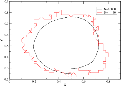
Figure 1: Stochastic motion around the fixed point, Moran process ($w=0.5$) for different population sizes. Shown is a phase space plot, where $x$ denotes the number of males in strategy A and $y$ denotes the number of females in strategy A. Due to the lack of helical paper, only one period of oscillation is shown. One can observe that for the large population ($N=10000$) the trajectory spirals inwards towards the fixed point at $(\frac{1}{2},\frac{1}{2})$.

The frequency-dependent Moran process (MO), and the other processes below (LU = local update TCH05 , FP = Fermi process TNP06 , and a linearized Moran process (LM) considered below) can more conveniently be written by means of a reproductive function

$$\Phi_{\rm MO}(\pi_{a},\langle\pi\rangle,w) = \frac{1}{2}\,\frac{1-w+w\pi_{a}}{1-w+w\langle\pi\rangle}$$ (23)

$$\Phi_{\rm LM}(\pi_{a},\langle\pi\rangle,w) = \frac{1}{2}(1+w(\pi_{a}-\langle\pi\rangle))$$ (24)

$$\Phi_{\rm LU}(\pi_{a},\pi_{b},w) = \frac{1}{2}(1+w(\pi_{a}-\pi_{b}))$$ (25)

$$\Phi_{\rm FP}(\pi_{a},\pi_{b},w) = \frac{1}{1+\exp(-w(\pi_{a}-\pi_{b}))}$$ (26)

so that the hopping probabilities are

$$T^{ba}=\Phi(\pi_{a},\pi_{b},w)\frac{N_{a}}{N}\frac{N_{b}}{N}$$ (27)

for the pairwise comparison processes (LU,FP), and

$$T^{ba}=\Phi(\pi_{a},\langle\pi\rangle,w)\frac{N_{a}}{N}\frac{N_{b}}{N}$$ (28)

for the other processes (MO,LM) where an individual’s payoff is compared to the payoff averaged over the whole population.

For all processes, $\Phi$ considers a two-particle (birth-death) process where an individual with fitness $\pi_{a}$ compares (Eqs. 23–24) with a representative sample of the population (i.e. the average fitness $\langle\pi\rangle$), or (Eqs. 25–26) with another individual $\pi_{b}$. The frequency-dependent Moran process moran ; nowak04 , the Local Update TCH05 , and the Fermi process TNP06 are microscopic evolutionary processes discussed recently. The Linearized Moran (LM) process arises as approximation of the Moran (MO) process in the weak selection limit $w\to 0$.

Note, that elsewhere for the Local update $w$ is replaced by $w/\Delta\pi_{\rm max}$, and for the Moran process, $w$ may not exceed $1-\pi_{\rm min}$. In the above notation, in the limit $w\to 0$ the Fermi process approaches the Local update process.

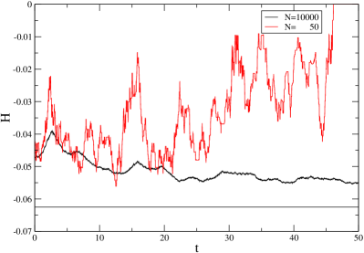
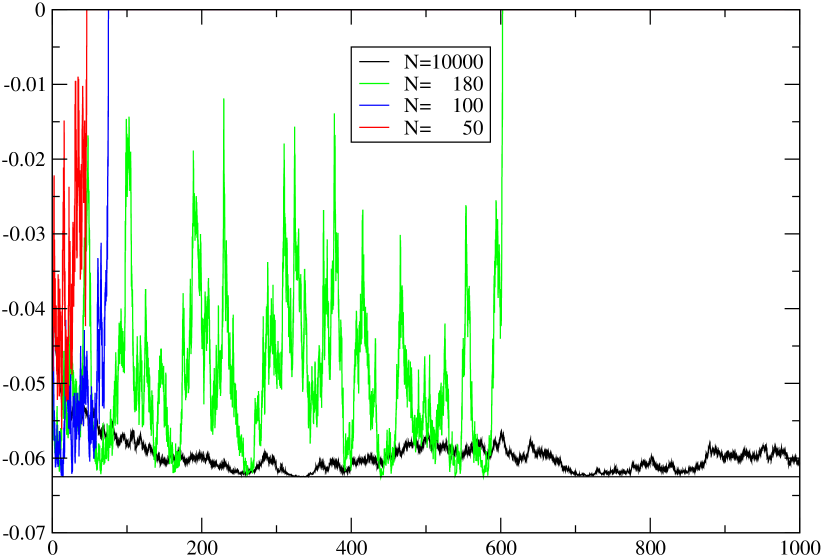
Figure 2: Stochastic motion around the fixed point, Moran process ($w=0.5$) for different population sizes (same as in Fig. 1). Here for the initial trajectory the value of $H$ (Eq. 17) is shown as a function of time. Time is measured in generation units, i.e. $N$ update steps are performed per unit time so that after $t=1$ each agent on average is updated once. For $N=50$, $H$ fluctuates and also increases on average (due to stochastic motion in the plane). For $N=10000$, $H$ decays as the trajectory approaches the fixed point. For the corresponding deterministic system, $H$ serves as a Lyapunov function of the stable fixed point and admits the value $H_{\rm fix}=-1/16$ there (straight line).

Figure 3: Stochastic motion around the fixed point. Moran process ($w=0.5$). For small population sizes, the internal fluctuations are large compared to the size of the phase space, hence fixation to the border is reached quickly. Above an intermediate range (in which the process behaves similar to neutral stable fixed point), fixation time diverges as the $N\to\infty$ behaviour of an asymptotically stable fixed point is recovered.

3 Stochastic motion around the fixed point

Having defined different possible microscopic update processes, one desires to gain an intuitive understanding of the resulting stochastic motion, in comparison of small (here, $N=50$) and large (here, $N=10000$) populations. Figure 1 compares the time evolution of the evolutionary trajectory in phase space $(x,y)$ and Figure 3 in the time evolution of $H$. For a large population, the qualitative dynamics of the adjusted replicator equation is recovered, i.e., convergence to the internal fixed point and thereby decrease of $H$ which serves as Lyapunov function in the deterministic limit. The motion of the small population is comparatively more stochastic, and after few generations, fixation to the border is reached. Intuitively, the “contracting force” of the stable fixed point is to weak to ensure the observation of a metastable state. Figure 3 shows a longer time interval and four different population sizes.

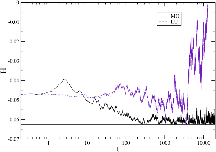
Figure 4: Stochastic motion around the fixed point. Time evolution over five decades for the Moran process (black) and the Local update process (red/gray) for a large population size $N=10000$ ($w=0.5$). For such large populations, the stochastic motion is close to the deterministic equations that follow in the limit $N\to\infty$ TCH05 . For the Local Update, the replicator equation is neutrally stable at the fixed point, and $H$ admits a constant of motion. The stochastic realization shows zero drift in $H$, but fluctuates, and ultimately the process leads to fixation to the border. Also the Moran process will reach the border for $t\to\infty$, however, after a long metastable transient. For the Moran process, the deterministic equation is the adjusted replicator equation which has an asymptotocally stable fixed point. Correspondingly $H$ decays describing a transient (metastable) attractive behaviour towards the fixed point. Note that due to the attracting force, the motion keeps confined to the vicinity of the fixed point and fluctuations are damped.

This paper addresses not only the influence of the population size, but also the influence of the microscopic update process. Figure 4 demonstrates that on longer time scales (here, the time scale is shown on a logarithmic scale to show the convergence behaviour). While the Local Update process performs a specific type of random walk in $H$ (in the sense that the internal fixed point is of neutral stability), the Moran process first confines the motion in the vicinity of the attracting internal point, but due to the discreteness of the process, fixates to the border in the limit $t\to\infty$. The initial conditions are the same as in the previous figures, starting from a state different from the fixed point, to show that the Moran process indeed leads to some type of convergence to the metastable state.

4 Deterministic and stochastic equations of motion at the level of the diffusion approximation

In many cases population sizes are such small that deviations from a deterministic population density cannot be neglected - especially because a species or genetic trait can go extinct, or likewise, a new mutant can either extinct or fixate (i.e., become the common trait in the whole population). If populations are not too small, e.g. $N=10^{2}$, one however can think of a perturbation expansion in orders of $1/N$ to derive stochastic corrections to the deterministic equations of motion. A classic approach in mathematical genetics in this direction is the so-called diffusion approximation crowkimura70 ; cherrywakely03 , which allows to derive fixation probabilities and densities from a Kolmogorov forward, or Fokker-Planck, equation. For a fixed population size and one trait (higherdimensional cases are prohibitive), the equivalence to a one-dimensional Markov chain allows for a closed exact expression.

A similar framework applies for deriving the equations of motion in zero and first order in $1/N$, and neglecting higher orders; i.e., we operate at the level of the diffusion approximation. Such approaches have been formulated in a wide range of fields from genetics to behavioural dynamics helbing92physicaa ; helbing96decision ; TCH05 ; TCH06 ; C08 ; crowkimura70 ; drosselreview . In the simplest setting of two strategies or traits, from the hopping rates $T^{+},T^{-}$ we have

$$\dot{\rho}(x,t)=-\nabla(a(x)\rho(x,t))+\nabla^{2}(b^{2}(x)\rho(x,t))$$ (29)

where $\nabla=\partial/\partial{}x$, $a(x)=T^{+}-T^{-}$ and $b^{2}(x)=(T^{+}+T^{-})/N$ have to be derived for each microscopic update process and payoff matrix.

4.1 Stability and drift reversal

The phase space average discussed in the next section can be interpreted as an approximation of the time evolution of an observable $H$, here, written for the case of two strategies only,

$$\dot{H}\simeq\langle\Delta H\rangle_{\rho x} := \!\!\int\!\!{\rm d}x\;\rho(x)\big{[}(H(x+1/N)\!-\!H(x))T^{+}$$ (30)

$$\hphantom{\int\!\!{\rm d}x\;\rho(x)\big{[}}\!\!\!\!\!\!\!\!\!+(H(x-1/N)\!-\!H(x))T^{-}\big{]}~{}~{}~{}~{}~{}$$

and, for an ensemble of arbitrary initial conditions, we approximate $\rho(x)$ by a constant. (Formally, one should distinguish between a continuous and a discrete phase space average; within this paper – apart from constant prefactors – the functions for $H$ and the rates $T$ are continuous and differentiable.)

In the remainder we focus on functions $H$ which also are Lyapunov functions of an internal fixed point. Then a decrease of $H$ can be interpreted as a motion towards the fixed point, and an increase of $H$ is interpreted as an escape from the fixed point. Thus we can define (omitting the subscript $x$ for the phase space average)

$$\langle\Delta H\rangle := \!\!\int\!\!{\rm d}x\big{[}(H(x+1/N)\!-\!H(x))T^{+}$$ (31)

$$\hskip 13.99995pt+(H(x-1/N)\!-\!H(x))T^{-}\big{]}$$

and define “drift reversal” as the change of sign of $\langle\Delta H\rangle$.

If a change of system parameters ($N,w$, payoffs), leads to a changing sign of $\langle\Delta H\rangle$, one observes the fixed point gradually lose its stochastic metastability. Due to this gradual transition, respective critical population sizes are approximative and could be defined in (possibly many) different ways. The essential advantage of assessing the stability from a sign reversal of this average drift $\langle\Delta H\rangle$ is that it can be calculated comparatively easy, and in the case of the Battle of the Sexes, even analytically.

5 Average drift: Battle of the Sexes

For the replicator equation, Eq. (17) defines a constant of motion. As we are interested in the finite-size corrections, we can use $H$ as an observable for the distance to the interior fixed point. For the processes defined above, the transition probabilities allow to calculate the average change of the constant of motion within the state space ($1\leq i,j\leq N-1$) as

$$\langle\Delta H\rangle = \frac{1}{N^{2}(N-1)^{2}}\sum_{i=1}^{N-1}\sum_{j=1}^{N-1}\Big{[}$$

$$i(N-i)j(N-j)(T^{+\bullet}+T^{-\bullet}+T^{\bullet+}+T^{\bullet-})$$

$$-(i+1)(N-i-1)j(N-j)T^{+\bullet}$$

$$-(i-1)(N-i+1)j(N-j)T^{-\bullet}$$

$$-i(N-i)(j+1)(N-j-1)T^{\bullet+}$$

$$-i(N-i)(j-1)(N-j+1)T^{\bullet-})\Big{]}$$

$$= \frac{1}{N^{2}(N-1)^{2}}\sum_{i=1}^{N-1}\sum_{j=1}^{N-1}\Big{[}$$

$$j(N-j)\big{[}(2i-N)(T^{+\bullet}-T^{-\bullet})+(T^{+\bullet}+T^{-\bullet})\big{]}$$

$$\!\!\!\!\!+i(N-i)\big{[}(2j-N)(T^{\bullet+}-T^{\bullet-})+(T^{\bullet+}+T^{\bullet-})\big{]}\Big{]}$$

$$= \frac{N^{2}}{(N-1)^{2}}\sum_{i=1}^{N-1}\sum_{j=1}^{N-1}\Big{[}$$

$$y(1-y)\big{[}\frac{2x-1}{N}(T^{+\bullet}-T^{-\bullet})\!+\!\frac{1}{N^{2}}(T^{+\bullet}+T^{-\bullet})\big{]}$$

$$\!\!\!\!\!+x(1-x)\big{[}\frac{2y-1}{N}(T^{\bullet+}-T^{\bullet-})\!+\!\frac{1}{N^{2}}(T^{\bullet+}+T^{\bullet-})\big{]}\Big{]}.$$

In the continuum limit the sums are replaced by integrals,

$$\langle\Delta H\rangle\! = \!\int_{0}^{1}\!{\rm d}x\int_{0}^{1}\!{\rm d}y\Big{[}$$

$$y(1-y)\big{[}\frac{2x-1}{N}(T^{+\bullet}-T^{-\bullet})\!+\!\frac{1}{N^{2}}(T^{+\bullet}+T^{-\bullet})\big{]}$$

$$\!\!\!\!\!+x(1-x)\big{[}\frac{2y-1}{N}(T^{\bullet+}-T^{\bullet-})\!+\!\frac{1}{N^{2}}(T^{\bullet+}+T^{\bullet-})\big{]}\Big{]}$$

$$= \!\frac{1}{N}\!\int_{0}^{1}\!{\rm d}x\int_{0}^{1}\!{\rm d}yx(1-x)y(1-y)\big{[}$$

$$\mbox{~{}~{}~{}~{}~{}~{}~{}~{}}(2x-1)(\Phi_{A}^{\text{\Male}}-\Phi_{B}^{\text{\Male}})+(2y-1)(\Phi_{A}^{\text{\Female}}-\Phi_{B}^{\text{\Female}})\big{]}$$

$$+\frac{1}{N^{2}}\int_{0}^{1}{\rm d}x\int_{0}^{1}{\rm d}yx(1-x)y(1-y)\big{[}$$

$$\mbox{~{}~{}~{}~{}~{}~{}~{}~{}~{}~{}~{}~{}~{}~{}~{}~{}~{}~{}~{}~{}~{}~{}~{}~{}~{}~{}~{}~{}~{}~{}~{}~{}}(\Phi_{A}^{\text{\Male}}+\Phi_{B}^{\text{\Male}}+\Phi_{A}^{\text{\Female}}+\Phi_{B}^{\text{\Female}})\big{]}$$

For given transition probabilities $T$ the drift of the discrete process can be expressed exactly, and in the case of linear processes, the resulting integrals are simple polynomial integrals. From this versatile expression, we can perform a comparison of the different processes.

5.1 Neutral evolution and Local Update

If $w=0$, or if all payoff elements are zero, all terms of type $(T^{+\bullet}-T^{-\bullet})$ vanish. Now consider the case where the payoffs come into play. For the Local Update, one has

$$\Phi_{A}^{\text{\Female}}+\Phi_{B}^{\text{\Female}}=\Phi_{A}^{\text{\Male}}+\Phi_{B}^{\text{\Male}}=1$$ (34)

and

$$\Phi_{A}^{\text{\Female}}-\Phi_{B}^{\text{\Female}} = -2w(2x-1)$$ (35)

$$\Phi_{A}^{\text{\Male}}-\Phi_{B}^{\text{\Male}} = +2w(2y-1).$$ (36)

Thus the term

$$(2x-1)(\Phi_{A}^{\text{\Male}}-\Phi_{B}^{\text{\Male}})+(2y-1)(\Phi_{A}^{\text{\Female}}-\Phi_{B}^{\text{\Female}})$$

vanishes identically, i.e. for the average drift for the local update as well as for neutral evolution only the $1/N^{2}$ order survives,

$$\langle\Delta H\rangle_{\rm LU} = \langle\Delta H\rangle_{\rm NE}=\frac{2}{N^{2}}\int_{0}^{1}{\rm d}x\int_{0}^{1}{\rm d}yx(1-x)y(1-y)$$ (37)

$$= \frac{1}{18N^{2}}.$$

The discrete stochastic diffusion in this neutral case is equivalent to the genetic drift of two independent types fisher ; wright and the $1/N$ term vanishes, as expected. But it is remarkable that the term in order $1/N$ does not contribute for the Local Update process. As this term corresponds for $N\to\infty$ to the ordinary replicator equation, this is fully consistent with $H$ being a constant of motion. For processes that depend on the payoff difference in a nonlinear manner, as the Fermi process, $H$ is no longer a constant of motion. However, the behaviour of $\langle\Delta H\rangle$ is remarkable, and investigated for finite populations in the next subsection.

5.2 General nonlinear pairwise comparison processes

Before approaching the nonlinear reproductive fitness defined by the frequency-dependent Moran process, it is instructive to analyze what happens if one considers a general pairwise comparison like for instance the Fermi process (26). Let us assume the general case that the difference between the reproductive functions $\Phi_{A}^{\text{\Female}}-\Phi_{B}^{\text{\Female}}$, which is antisymmetric upon interchanging the strategies $A,B$ of the individuals anyhow, merely is a function of the difference of the payoffs

$$\Phi_{A}^{\text{\Female}}-\Phi_{B}^{\text{\Female}}=:f(\pi_{A}^{\text{\Female}}-\pi_{B}^{\text{\Female}}),$$ (38)

which is fulfilled for the Local update, the Fermi process, and practically all common local comparison processes including “Imitate if Better”. Then $f$ is odd, $f(x)=-f(-x)$. We also assume that this function is identical for the female and male population – this is justified as those differences should be cast into the payoff matrix rather than manipulating the reproductive functions. For convenience, one can here require $f$ to be infinitely differentiable. Then $f$ has only odd Taylor coefficients,

$$\Phi_{A}^{\text{\Female}}-\Phi_{B}^{\text{\Female}} = f(\pi_{A}^{\text{\Female}}-\pi_{B}^{\text{\Female}})=f(\Delta\pi)$$

$$= f^{{}^{\prime}}\Delta\pi+\frac{f^{{}^{\prime\prime\prime}}}{3!}(\Delta\pi)^{3}+\frac{f^{(5)}}{5!}(\Delta\pi)^{5}+\ldots$$

The linear term is that of the Local update, whose cancellation in $\langle\Delta H\rangle$ we have seen before. Upon inspection of, e.g., the order $(2n+1)$ term, one finds apart from common factors $H{f^{(2n+1)}}/{(2n+1)!}$ that the integrand contains

$$(2x-1)(2(2y-1))^{2n+1}+(2y-1)(-2(2x-1))^{2n+1}$$

$$=2^{2n+1}(2x-1)(2y-1)\big{(}(2y-1)^{2n}-(2x-1)^{2n}\big{)}$$

That is, for every $n$, the integral in order $1/N$ splits into the difference between two integrals which are symmetric in interchange of $x$ and $y$, thus identical, and the contributions of each Taylor coefficient cancel. Hence follows

Theorem 5.1

For a pairwise-type comparison process, where the difference between reproductive fitnesses $\Phi_{A}-\Phi_{B}$ is an infinitely differentiable function of the payoff difference, the average drift $\langle\Delta H\rangle$ in the Battle of the Sexes (with the $\pm 1$ payoff matrix) is independent of the strength of selection $w$ and equal to the drift of neutral evolution (37).

As a corollary, there is no drift reversal for the Local update as well as for the Fermi process, confirming the numerical results in TCH05 ; CT06 .

The result is remarkable in one sense. Even though a nonlinear comparison process can lead to a nonlinear replicator equation – which e.g. takes the form of a tangens hyperbolicus of the payoff difference for the Fermi process TNP06 – the average drift remains unaffected even for strong selection and small populations.

5.3 Linearized Moran process

For the linearized Moran process, one has

$$\Phi_{A}^{\text{\Female}}+\Phi_{B}^{\text{\Female}}=1+\frac{w}{2}(\pi_{A}^{\text{\Female}}+\pi_{B}^{\text{\Female}}-2\langle\pi^{\text{\Female}}\rangle);$$ (39)

for the male population a corresponding equation holds. The integrand in the diffusion (order $1/N^{2}$) term, apart from a factor $H$, is

$$2+\frac{w}{2}(\pi_{A}^{\text{\Female}}+\pi_{B}^{\text{\Female}}+\pi_{A}^{\text{\Male}}+\pi_{B}^{\text{\Male}}-2\langle\pi^{\text{\Female}}\rangle-2\langle\pi^{\text{\Male}}\rangle).$$

As the sum of the payoffs $A$ and $B$ is zero for both populations, and

$$\langle\pi^{\text{\Female}}\rangle=y(1-2x)+(1-y)(2x-1)=-(2x-1)(2y-1)$$

$$=-x(2y-1)+(1-x)(2y-1)=-\langle\pi^{\text{\Male}}\rangle,$$

again the game does not contribute to the diffusion term, which is, independently of $w$, identical to the neutral case. Now, does the game contribute to the first order? Here,

$$\Phi_{A}^{\text{\Female}}-\Phi_{B}^{\text{\Female}} = -\frac{w}{2}(\pi_{A}^{\text{\Female}}-\pi_{B}^{\text{\Female}})=-w(2x-1)$$ (40)

$$\Phi_{A}^{\text{\Male}}-\Phi_{B}^{\text{\Male}} = +\frac{w}{2}(\pi_{A}^{\text{\Male}}-\pi_{B}^{\text{\Male}})=+w(2y-1)$$ (41)

and thus again the term

$$(2x-1)(\Phi_{A}^{\text{\Male}}-\Phi_{B}^{\text{\Male}})+(2y-1)(\Phi_{A}^{\text{\Female}}-\Phi_{B}^{\text{\Female}})$$

vanishes, i.e. for the average drift for the local update as well as for neutral evolution only the $1/N^{2}$ order survives,

$$\langle\Delta H\rangle_{\rm LM} = \frac{1}{18N^{2}}.$$

5.4 Moran process

For the Moran process, it is possible to proceed even despite the nonlinearities. The Moran payoffs are, e.g. for males in strategy A,

$$\Phi^{A}_{\text{\Male}} = \frac{1}{2}\frac{1-w+w\pi^{A}_{\text{\Male}}}{1-w+w\langle\pi_{\text{\Male}}\rangle}.$$

Using $\pi^{A}_{\text{\Male}}+\pi^{B}_{\text{\Male}}=0$, and $\langle\pi_{\text{\Female}}\rangle+\langle\pi_{\text{\Male}}\rangle=0$, it follows

$$\Phi^{A}_{\text{\Male}}+\Phi^{B}_{\text{\Male}}+\Phi^{A}_{\text{\Female}}+\Phi^{B}_{\text{\Female}}$$

$$= \hphantom{+}\frac{1}{2}\frac{(1-w+w\pi^{A}_{\text{\Female}})(2-2w+w\pi^{A}_{\text{\Male}}+w\pi^{B}_{\text{\Male}})}{(1-w+w\langle\pi_{\text{\Male}}\rangle)(1-w+w\langle\pi_{\text{\Female}}\rangle)}$$

$$+\frac{1}{2}\frac{(1-w+w\pi^{A}_{\text{\Male}})(2-2w+w\pi^{A}_{\text{\Female}}+w\pi^{B}_{\text{\Female}})}{(1-w+w\langle\pi_{\text{\Male}}\rangle)(1-w+w\langle\pi_{\text{\Female}}\rangle)}$$

$$= \frac{2(1-w)^{2}}{(1-w)^{2}-w^{2}\langle\pi_{\text{\Female}}\rangle^{2}}.$$

In the weak selection limit, $w\to 0$, this term approximates the constant 2. For $w\to 1$, it vanishes asymptotically, but is negative for $\frac{1}{2}<w<1$, due to a pole at $w=\frac{1}{2}$. While for $x=\frac{1}{2}$ or $y=\frac{1}{2}$ (a cross of lines in the state space) the average fitness vanishes, in the corners the square of the average fitness always is $1$.

The difference terms in the reproductive functions are

$$\Phi^{A}_{\text{\Male}}-\Phi^{B}_{\text{\Male}} = \frac{1}{2}\frac{w(\pi^{A}_{\text{\Male}}-\pi^{B}_{\text{\Male}})}{1-w+w\langle\pi_{\text{\Male}}\rangle}=+\frac{w(2y-1)}{1-w+w\langle\pi_{\text{\Male}}\rangle}$$

$$\Phi^{A}_{\text{\Female}}-\Phi^{B}_{\text{\Female}} = \frac{1}{2}\frac{w(\pi^{A}_{\text{\Female}}-\pi^{B}_{\text{\Female}})}{1-w+w\langle\pi_{\text{\Female}}\rangle}=-\frac{w(2x-1)}{1-w+w\langle\pi_{\text{\Female}}\rangle}.$$

The $1/N$ term thus becomes, observing $\langle\pi_{\text{\Female}}\rangle=-\langle\pi_{\text{\Male}}\rangle$,

$$\frac{w}{N}\int_{0}^{1}{\rm d}x\int_{0}^{1}{\rm d}yx(1-x)y(1-y)$$

$$\mbox{~{}~{}~{}~{}~{}~{}~{}~{}~{}~{}~{}~{}~{}~{}~{}}\times\Big{[}\frac{(2x-1)(2y-1)}{1-w+w\langle\pi_{\text{\Male}}\rangle}-\frac{(2x-1)(2y-1)}{1-w-w\langle\pi_{\text{\Male}}\rangle}\Big{]}$$

$$= \frac{w}{N}\int_{0}^{1}{\rm d}x\int_{0}^{1}{\rm d}yx(1-x)y(1-y)(2x-1)(2y-1)$$

$$\mbox{~{}~{}~{}~{}~{}~{}~{}~{}~{}~{}~{}~{}~{}~{}~{}}\times\frac{(1-w-w\langle\pi_{\text{\Male}}\rangle)-(1-w+w\langle\pi_{\text{\Male}}\rangle)}{(1-w)^{2}-w^{2}\langle\pi_{\text{\Male}}\rangle^{2}}$$

$$= \frac{w}{N}\int_{0}^{1}{\rm d}x\int_{0}^{1}{\rm d}yx(1-x)y(1-y)(2x-1)(2y-1)$$

$$\mbox{~{}~{}~{}~{}~{}~{}~{}~{}~{}~{}~{}~{}~{}~{}~{}}\times\frac{-2w\langle\pi_{\text{\Male}}\rangle}{(1-w)^{2}-w^{2}\langle\pi_{\text{\Male}}\rangle^{2}}.$$

The average drift for the Moran process then reads

$$\langle\Delta H\rangle_{\rm MO} = \int_{0}^{1}{\rm d}x\int_{0}^{1}{\rm d}y\frac{x(1-x)y(1-y)}{(1-w)^{2}-w\langle\pi^{\text{\Male}}\rangle^{2}}$$

$$\times\Big{[}\frac{2(1-w)^{2}}{N^{2}}-\frac{2w^{2}\langle\pi^{\text{\Male}}\rangle(2x-1)(2y-1)}{N}\Big{]}$$

$$= 2\int_{0}^{1}{\rm d}x\int_{0}^{1}{\rm d}y\frac{x(1-x)y(1-y)}{(1-w)^{2}-w\langle\pi^{\text{\Male}}\rangle^{2}}$$

$$\mbox{~{}~{}~{}~{}~{}~{}~{}~{}~{}~{}~{}~{}~{}~{}~{}~{}~{}}\times\frac{2(1-w)^{2}-Nw^{2}\langle\pi^{\text{\Male}}\rangle^{2}}{N^{2}}$$

$$= \frac{2}{N^{2}}\int_{0}^{1}{\rm d}x\int_{0}^{1}{\rm d}yx(1-x)y(1-y)$$

$$\mbox{~{}~{}~{}~{}~{}~{}~{}~{}~{}~{}~{}~{}~{}~{}~{}~{}~{}~{}~{}~{}}\times\frac{(1-w)^{2}-Nw^{2}\langle\pi^{\text{\Male}}\rangle^{2}}{(1-w)^{2}-w^{2}\langle\pi^{\text{\Male}}\rangle^{2}}.$$

For weak selection $w\ll\frac{1}{2}$, and $N\gg 1$, one can approximate the last fraction, yielding

$$\langle\Delta H\rangle_{\rm MO} \simeq \frac{2}{N^{2}}\int_{0}^{1}{\rm d}x\int_{0}^{1}{\rm d}yx(1-x)y(1-y)$$

$$\mbox{~{}~{}~{}~{}~{}~{}~{}~{}~{}~{}~{}~{}~{}~{}~{}~{}}\times[1-Nw^{2}(2x-1)^{2}(2y-1)^{2})].$$

Weak selection limit of the drift for the Moran process

Despite reproductive success is based on a comparison with the average payoff (instead of a pairwise comparison), for the linearized Moran process investigated in Section 5.3, the drift reversal is lost. Thus, performing the weak selection limit at the level of the microscopic interaction does not properly conserve the properties of the average drift of the frequency-dependent Moran process. But from the exact theory for the Moran case, one can consider the approximation $w\to 0$ at a later stage:

$$\langle\Delta H\rangle_{\rm MO} \simeq -\frac{1}{N}\int_{0}^{1}{\rm d}x\int_{0}^{1}{\rm d}y\,\,2w^{2}x(1-x)y(1-y)$$ (43)

$$\mbox{~{}~{}~{}~{}~{}~{}~{}~{}~{}~{}~{}~{}~{}~{}~{}~{}~{}~{}~{}~{}~{}~{}~{}~{}~{}}\times(2x-1)^{2}(2y-1)^{2}$$

$$+\frac{2}{N^{2}}\int_{0}^{1}{\rm d}x\int_{0}^{1}{\rm d}yx(1-x)y(1-y)$$

$$= -\frac{2w^{2}}{900N}+\frac{1}{18N^{2}}.$$

Both terms cancel for a $w$ that matches

$$N_{c}=25/w^{2}.$$ (44)

One should bear in mind that due to the approximation $w\ll 1/2$ made above, equations (43) and (44) rely on the weak selection limit, which is the biologically most relevant case.

An interesting viewpoint on its own is to consider $w$ as a “bifurcation” parameter. Conversely to a Hopf bifurcation, where an oscillation amplitude grows with the square root of a bifurcation parameter, here the effect of the Moran dynamics, to stabilize the finiteness-stochastic oscillations around the fixed point, grows quadratically with the strength of selection $w$. Thus, for the frequency-dependent Moran process in finite populations, the onset of the fixed-point stabilizing mechanism is a quadratic effect of weak, but increasing, selection.

6 Discussion

The investigation of the different update mechanisms suggests the existence of two universality classes: one, for which the internal fixed point is neutrally stable (in the $N\to\infty$ limit), and a second, for which the internal fixed point is asymptotically stable (in the $N\to\infty$ limit).

The Local update process as well as other (differentiable and pair-symmetric) pairwise comparison processes, as the Fermi process, and also a linearized Moran process, belong to the first class. The Moran process belongs to the second class, and one may assume that more update processes (combining average fitness and a nonlinearity) could be constructed for this class; the necessary condition is that the internal fixed point is attractive in the $N\to\infty$ limit.

In this sense, the properties that were known for the deterministic replicator equations were recovered, and for the Moran process class the transition between the instable and (meta-) stable regime can be described by calculating the drift reversal from $\langle\Delta H\rangle$. This approach may be advantageous in high-dimensional cases, where exact simulations of the process become costly; a phase space average of $\langle\Delta H\rangle$ is obtained much easier, and in very high dimensional spaces one may approximate by a Monte Carlo integration.

7 Conclusions

Cyclic coevolution in biological or social dynamics is an interesting class of coevolutionary dynamics and allows in an examplaric way to study stability, drift and diffusion in finite populations. Population sizes in markets, decison processes, as well as in biological populations from bacteria to ants and to vertebrates can vary by many orders of magnitude, thus the influence of the population size by the stochasticity in finite populations is of fundamental relevance in all those disciplines.

For the simplest generic model of a cyclic coevolution in an asymmetric conflict game between two populations, the “Battle of the Sexes”, analytical results for the average drift could be obtained that support the consistent understanding how the different fixed point stability of ordinary and adjusted replicator equations translate to finite populations.

Partially the results are quite unexpected: Not only for the Fermi process, but also for a quite general class of pairwise comparison processes – even when they lead to different replicator equations – the average drift is identical to the neutral case, and equals $1/(18N^{2})$. The second surprise is that, for the average drift, the linearized Moran process also falls into the equivalence class of the neutral evolution.

But how does the drift reversal seen numerically (and known in the $N\to\infty$ limit for the adjusted replicator equation) then have to be explained? Here one has to calculate the average drift for the Moran case, using the nonlinear dependence on the average payoff to observe the drift reversal. The hereby obtained average drift then can be analyzed for weak selection, resulting in an estimate of the critical population size which delimits the stability regimes of ordinary and adjusted replicator equations.

More generally speaking, one can conclude that, to stabilize the coexistence of strategies in a large – but finite – population, not only the global knowledge of the overall success of the population – the average payoff – must be taken into account, but in addition it has to determine the reproductive fitness in a nonlinear manner. The (on process level) linearized Moran process, as well as neutral evolution or pairwise comparison, leads to quicker extinction of all but one of the four strategy pairs.

References

- (1) B. Kerr, M.A. Riley, M.W. Feldman, and B.J.M. Bohannan, Local dispersal promotes biodiversity in a real-life game of rock-paper-scissors, Nature 418, 171 (2002).
- (2) B.C. Kirkup and M.A. Riley, Antibiotic-mediated antagonism leads to a bacterial game of rock-paper-scissors in vivo, Nature 428, 412 (2004).
- (3) M. Eigen, P. Schuster, The Hypercycle, Naturwissenschaften 65, 7 (1978).
- (4) B. Sinervo, C.M. Lively, The rock-paper-scissors game and the evolution of alternative male strategies, Nature 380, 240 (1996).
- (5) K.R. Zamudio and B. Sinervo, Polygyny, mate-guarding, and posthumous fertilization as alternative male mating strategies, PNAS 97, 14427 (2000).
- (6) B. Sinervo, Runaway social games, genetic cycles driven by alternative male and female strategies, and the origin of morphs, Genetica 112, 417 (2001).
- (7) Dirk Helbing, Interrelations between stochastic equations for systems with pair interactions, Physica A 181, 29-52 (1992). – cond-mat/9805256
- (8) Dirk Helbing, Stochastic and Boltzmann-like models for behavioral changes, and their relation to game theory, Physica A 193, 241-258 (1993). – cond-mat/9805293
- (9) Dirk Helbing, Boltzmann-like and Boltzmann-Fokker-Planck equations as a foundation of behavioral models, Physica A 196, 546-573 (1993). – cond-mat/9805384
- (10) Dirk Helbing, Martin Treiber, and Nicole J. Saam, Analytical investigation of innovation dynamics considering stochasticity in the evaluation of fitness, Phys. Rev. E 71, 067101 (2005).
- (11) D. Helbing, A mathematical model for the behavior of individuals in a social field, Journal of Mathematical Sociology 19, 189 (1994). – cond-mat/9805194
- (12) Dirk Helbing, A Mathematical Model for Behavioral Changes by Pair Interactions and Its Relation to Game Theory, Angewandte Sozialforschung 18 (3), 117-132 (1994). – cond-mat/9805102
- (13) D. Helbing, A stochastic behavioral model and a “microscopic” foundation of evolutionary game theory, Theory and Decision 40, 149-179 (1996). – cond-mat/9805340
- (14) C. Hauert, S. De Monte, J. Hofbauer, K. Sigmund, Volunteering as Red Queen Mechanism for Cooperation in Public Goods Games, Science 296, 1129 (2002).
- (15) György Szabó and Christoph Hauert, Phase Transitions and Volunteering in Spatial Public Goods Games, Phys. Rev. Lett. 89, 118101 (2002).
- (16) M. A. Nowak, Evolutionary Dynamics, Harvard University Press (2006).
- (17) G. Szabo and G. Fath, Evolutionary games on graphs, Physics Reports 446, 97 (2007). – cond-mat/0607344
- (18) Jacek Miekisz, Evolutionary game theory and population dynamics, q-bio/0703062, (to appear in: Lecture Notes in Mathematics).
- (19) Richard Dawkins, The Selfish Gene, Oxford UP (1976).
- (20) J. Hofbauer, K. Sigmund, Evolutionary Games and Population Dynamics, Cambridge University Press (1998).
- (21) Anne E. Magurran and M. A. Nowak, Another Battle of the Sexes: The Consequences of Sexual Asymmetry in Mating Costs and Predation Risk, Proc. Roy. Soc. B 246, 31 (1991).
- (22) P. A. P. Moran, The Statistical Processes of Evolutionary Theory, Clarendon, Oxford (1962).
- (23) M. A. Nowak, A. Sasaki, C. Taylor, and D. Fudenberg, Emergence of cooperation and evolutionary stability in finite populations, Nature 428, 646 (2004).
- (24) C. Taylor, D. Fudenberg, A. Sasaki, and M. A. Nowak, Evolutionary game dynamics in finite populations, Bull. Math. Biol. 66, 1621 (2004).
- (25) A. Traulsen, J.C. Claussen, and C. Hauert, Coevolutionary Dynamics: From Finite to Infinite Populations, Phys. Rev. Lett. 95, 238701 (2005).
- (26) J.C. Claussen and A. Traulsen, Non-Gaussian fluctuations arising from finite populations: Exact results for the evolutionary Moran process, Phys. Rev. E 71, 025101(R) (2005).
- (27) A. Traulsen, J.C. Claussen, and C. Hauert, Coevolutionary dynamics in large, but finite populations, Phys. Rev. E 74, 011901 (2006).
- (28) T. Reichenbach, M. Mobilia, E. Frey, Coexistence versus extinction in the stochastic cyclic Lotka-Volterra model, Physical Review E 74, 051907 (2006).
- (29) J. C. Claussen and A. Traulsen, Fluctuations in Coevolutionary Dynamics and Implications for Multi-Agent Models, p. 411-419, in: Dirk Helbing (Ed.), Proc. Potentials of Complexity Science for Business, Government, and the Media, Budapest (2006).
- (30) J. C. Claussen, Discrete stochastic processes, replicator and Fokker-Planck equations of coevolutionary dynamics in finite and infinite populations, Banach Center Publications, to be published (2008).
- (31) L. E. Blume, The statistical Mechanics of Best-Response Strategy Revision, Games Econ. Behav. 11, 111-145 (1995).
- (32) Arne Traulsen, Martin A. Nowak, and Jorge M. Pacheco, Stochastic dynamics of invasion and fixation, Phys. Rev. E 74, 011909 (2006).
- (33) J. F. Crow and M. Kimura, Introduction to Population Genetics Theory, Harper & Row, New York, 1970.
- (34) J. L. Cherry, J. Wakely, A diffusion approximation for selection and drift in a subdivided population, Genetics 163, 421 (2003).
- (35) B. Drossel, Biological Evolution and Statistical Physics, Advances in Physics 50, 209 (2001). – cond-mat/0101409
- (36) R. A. Fisher The Genetical Theory of Natural Selection, Oxford University Press, Oxford. Dover, New York (1930).
- (37) S. Wright, Evolution in Mendelian populations, Genetics 16, 97 (1931).