Cyclotron radiation and emission in graphene

Abstract

Peculiarity in the cyclotron radiation and emission in graphene is theoretically examined in terms of the optical conductivity and relaxation rates to propose that graphene in magnetic fields can be a candidate to realize the Landau level laser, proposed decades ago [H. Aoki, Appl. Phys. Lett. 48, 559 (1986)].

Introduction — There has been an increasing fascination with the physics of graphene, a monolayer of graphite, as kicked off by the experimental discovery of an anomalous quantum Hall effect(QHE).Nov05 ; Zhang et al. (2005) The fascination comes from a condensed-matter realization of the massless Dirac-particle dispersion at low energy scales on the honeycomb lattice,McClure (1956); Zheng and Ando (2002); Gusynin and Sharapov (2005); Nov05 ; Peres et al. (2006) which is behind all the peculiar properties of graphene. In magnetic fields this appears as unusual Landau levels, where (i) the Landau levels ($=\sqrt{n}\hbar\omega_{c}$, $n$: Landau index) are unevenly spaced, (ii) the cyclotron frequency $\omega_{c}=(2e/c\hbar)v_{F}\sqrt{B}$ is proportional to $\sqrt{B}$ rather than to $B$, and (iii) there is an extra Landau level right at the massless Dirac point ($E=0$), which is outside the Onsager’s semiclassical quantization.Onsager (1952) While various transport measurements, as exemplified by the quantum Hall effect, have been extensively done, optical properties are also measured. For example, Sadowski et al have performed a Landau level spectroscopy for a large graphene sample. Inter-Landau level transitions are observed at multiple energies, which is due to a peculiar optical selection rule ($|n|\leftrightarrow|n|+1$ as opposed to the usual $n\leftrightarrow n+1$) as well as to the uneven Landau levels.

Now, if we look at the QHE physics, cyclotron emission from the QHE system in non-equilibrium has been one important phenomenon. Experimentally, this typically appears as a strong cyclotron emission from the “hot spot”, a singular point in a Hall-bar sample where the convergence of electric lines of force puts the electrons out of equilibrium.Ikushima et al. (2004) Theoretically, one of the present authors proposed a “Landau-level laser” for non-equilibrium QHE systems.Aoki (1986) The basic idea is simple enough: we can exploit the unusual coalescence of the energy spectrum into a series of line spectrum (Landau levels) realize a laser from a spontaneous emission if we can make a population inversion, where the photon energy (= cyclotron energy in this case) is tunable and falls on the terahertz region for $B\sim 10$T. However, the most difficult part is the population inversion, since if we e.g. optically pump the system, the excitation would go up the ladder of equidistant Landau levels indefinitely.

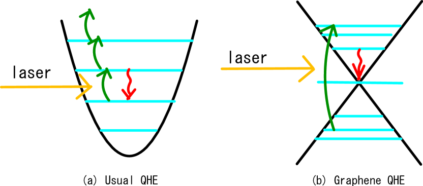
Figure 1: (Color online) Cyclotron absorption (green) and emission (red) processes schematically depicted for the ordinary(a) and graphene(b) quantum Hall systems. Black lines represent the band dispersion, while blue lines Landau levels.

This has motivated us to put a question (Fig.1): will the graphene Landau levels, with uneven spacing among their peculiarities, favor in realizing such a population inversion? In this Letter we show that this is indeed the case, by actually calculating the optical conductivity as well as the relaxation processes. The message here is graphene is a candidate for the Landau-level laser.

Optical conductivity in graphene — Low-energy physics around the Fermi energy in graphene is described by the massless Dirac Hamiltonian,Zheng and Ando (2002)

$$H_{0}=v_{F}\begin{pmatrix}0&\pi^{-}&0&0\\ \pi^{+}&0&0&0\\ 0&0&0&\pi^{+}\\ 0&0&\pi^{-}&0\\ \end{pmatrix},$$ (1)

where $v_{F}$ is the velocity at $E_{F}$, $\pi^{\pm}\equiv\pi_{x}\pm i\pi_{y}$, $\mbox{\boldmath$\pi$}={\bf p}+e{\bf A}$, ${\bf A}$ the vector potential representing a uniform magnetic field ${\bf B}={\rm rot}{\bf A}$, and the $4\times 4$ matrix is spanned by the chirality and (K, K’) Fermi points. In magnetic fields the energy spectrum is quantized into Landau levels,

$$\varepsilon_{n}={\rm sgn}(n)\sqrt{n}\hbar\omega_{c},$$ (2)

$$\omega_{c}=\frac{\sqrt{2}}{\ell}v_{F}=v_{F}\sqrt{\frac{2eB}{\hbar}},$$ (3)

for a clean system, where $n=0,\pm 1,...$ is the Landau index, and $\ell=\sqrt{\hbar/eB}$ the magnetic length. Here we consider realistic systems having disorder with the self-consistent Born approximation (SCBA) introduced by AndoAndo (1975); Zheng and Ando (2002) to calculate the optical conductivity.

The optical conductivity is given by

$$\begin{split}\sigma_{\alpha\beta}&(\omega)=\frac{e^{2}\hbar}{i\pi}\int d\varepsilon\frac{f(\varepsilon)}{\hbar\omega}\\ &\times\left[\mbox{Tr}\left(j_{\alpha}{\rm Im}G(\varepsilon)j_{\beta}(G^{+}(\varepsilon+\hbar\omega)-G^{+}(\varepsilon))\right)\right.\\ &\hskip 10.00002pt\left.-\mbox{Tr}\left(j_{\alpha}(G^{-}(\varepsilon)-G^{-}(\varepsilon-\hbar\omega))j_{\beta}{\rm Im}G(\varepsilon)\right)\right],\end{split}$$ (4)

where $\alpha,\beta=x,y$, $f(\varepsilon)$ the Fermi distribution, and $G^{\pm}=G(\epsilon\pm i\delta)$. For Green’s function $G$, with the self-energy $\Sigma_{n}(\varepsilon)=\Gamma\sum_{n^{\prime}}[\varepsilon-{\rm sgn}(n)\sqrt{|n|}-\Sigma_{n^{\prime}}(\varepsilon)]^{-1}$ in the SCBA, the Landau level broadening is given by $\Gamma=n_{0}V_{0}^{2}$ if we assume for simplicity short-ranged random potential, $V=\sum_{i}V_{0}\delta({\bf r}-{\bf r}_{i})$. The light absorption rate is then related to the imaginary part of the dielectric function, $\varepsilon(\omega)=1+i\sigma_{xx}(\omega)/\varepsilon_{0}\omega,$ so we can look at $\mbox{Re}\,\sigma_{xx}(\omega)$.

In order to discuss the optical conductivity in graphene we need the current matrix elements across Landau levels. The eigenfunctions of the Hamiltonian (1) dictate an unusual selection rule, $|n|-|n^{\prime}|=\pm 1$ in place of the ordinary $n-n^{\prime}=\pm 1$, withAndo (1975)

$$j_{x}^{n,n^{\prime}}=v_{F}C_{n}C_{n^{\prime}}\left[{\rm sgn}(n)\delta_{|n|-1,|n^{\prime}|}+{\rm sgn}(n^{\prime})\delta_{|n|+1,|n^{\prime}|}\right],$$

$$j_{y}^{n,n^{\prime}}=iv_{F}C_{n}C_{n^{\prime}}\left[{\rm sgn}(n)\delta_{|n|-1,|n^{\prime}|}-{\rm sgn}(n^{\prime})\delta_{|n|+1,|n^{\prime}|}\right],$$ (5)

where $C_{n}=1(n=0)$ or $1/\sqrt{2}$ (otherwise).

We have numerically obtained the Green’s function and optical conductivity. While in usual cases the broadened Landau levels are uniformly merged or separated as $\Gamma$ is varied, there is a striking difference for graphene, where the Landau levels ($\propto\sqrt{n}$) are unevenly spaced, so that the broadened Landau levels overlap to lesser extent as we go to the central one ($n\rightarrow 0$), as typically depicted in Fig.2. Namely, for an intermeditate value of $\Gamma/\omega_{c}$ only the $n=0$ Landau level stands alone while the other levels form a continuous spectrum.

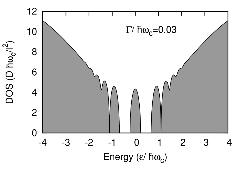
Figure 2: A typical density of states for graphene for an intermediate disorder ($\Gamma/\omega_{c}=0.03$ here).

We now look at the optical conductivity in Fig.3 for the Fermi energy at $\varepsilon_{F}=0$ (energy for the Dirac point), each resonance peak can be assigned to an allowed transition with the selection rule (eqn(5)). The largest peak around $\omega/\omega_{c}=1$ corresponds to the transition between $n=0\leftrightarrow\pm 1$, while the peaks at higher frequencies come from the transition across the Fermi energy, $-n\leftrightarrow n\pm 1$. If we turn to the temperature dependence in the figure, we immediately notice a peculiar phenomenon: there is a peak, in the region $\omega/\omega_{c}<1$, that grows, rather than decays, for higher $T$. We can identify this as coming from the unusual Landau levels in graphene: As $T$ is raised with the Fermi distribution function becoming longer-tailed, higher Landau levels begin to be occupied, which enables the transitions among higher Landau levels, $n\leftrightarrow n\pm 1$, to take place. While this would not cause new lines to appear for equidistant Landau levels, this does so for the unequally spaced Landau levels ($\propto\sqrt{|n|}$) for $\omega/\omega_{c}<1$ transitions. So we can identify this property as one hallmark of the “massless Dirac” dispersion.

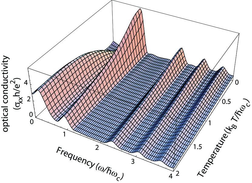
Figure 3: (Color online) Optical conductivity against $\omega$ is shown for temperatures $k_{B}T/\hbar\omega_{c}=0-2.0$, for a fixed value of $\Gamma/\hbar\omega_{c}=0.01$ with $\varepsilon_{F}=0$.

Previously, the optical conductivity has been obtained by Gusynin et al,Gusynin et al. (2007)Gusynin and Sharapov (2006) who have derived the analytical expression for the optical conductivity, but the self-energy from the disorder was set to a constant, while we have calculated the self-energy self-consistently with SCBA. Sadowski et al.Sadowski et al. (2006) also presented a similar expression for the conductivity with a constant self-energy as well. The present result qualitatively agrees with these, but the new findings here are, first, the full dependence on the $k_{B}T/\hbar\omega_{c}$, including the growing of low-frequency peaks at low temperatures. Secondly, we point out that the situation as depicted in Fig.2 should be interesting for the cyclotron resonance and emission in non-equilibrium situations induced by e.g. an optical pumping with laser beams. Namely, the electrons excited to higher energies will relax down to the $n=1$ level across the continuum spectrum, so that the population inversion across $n=0$ and $n\geq 1$ should be easier to be realized.

Relaxation processes — To quantify this idea, we have to consider the relaxation processes which should control the population inversion. For the ordinary quantum Hall systems the relaxation processes have been extensively discussed. Specifically, Chaubet et al.Chaubet et al. (1995)Chaubet and Geniet (1998) discussed dissipation mechanisms, where spontaneous photon radiation and coupling with phonons are examined on the basis of Fermi’s golden rule. Other dissipation processes such as electron-electron scattering or impurity scattering, which conserve the total energy, do not contribute to inter-Landau level processes in the absence of external electric fields (while Chaubet et al. have focused on effects of finite electric fields in the QHE breakdown where inter-Landau level processes are involved).

So we extend the discussion by Chaubet et al. to relaxation processes in graphene. We first estimate the efficiency of the photon emission with Fermi’s golden rule:

$$W_{i\to f}=\frac{2\pi}{\hbar}|\langle i|H_{\rm int}|f\rangle|^{2}\delta(\epsilon_{f}-\epsilon_{i}).$$

Here $|i\rangle(\epsilon_{i})$ is the wavefunction (energy) in the initial state while f stands for the final states, and $H_{\rm int}$ the electric dipole interaction between the electromagnetic field and electrons. When the wavelength of light is much larger than the cyclotron radius, as is usually the case, we have

$$W_{i\rightarrow f} = \frac{2\pi}{\hbar}\frac{V}{\pi^{2}c^{3}}\int\omega^{\prime 2}d\omega^{\prime}\frac{e^{2}\hbar}{2\epsilon_{0}V\omega^{\prime}}|\langle i|v|f\rangle|^{2}$$ (6)

$$\times \delta(\hbar\omega^{\prime}+\epsilon_{f}-\epsilon_{i})=4\alpha\left(\frac{|\langle i|v|f\rangle|}{c}\right)^{2}\omega,$$

where $c$ is the velocity of light, $\alpha=e^{2}/(4\pi\epsilon_{0}\hbar c)$ the fine-structure constant, and we put $\hbar\omega=\epsilon_{f}-\epsilon_{i}$ to be the cyclotron energy $\hbar\omega_{c}$.

A peculiarity of graphene appears in the current matrix element (eqn(5)), for which the rate of spontaneous emission, with $|\langle n|v|n+1\rangle|=C_{n}C_{n+1}v_{F}$ for graphene plugged in, reads

$$W_{n+1\to n}^{\rm graphene}=\begin{cases}2\alpha\left(\frac{v_{F}}{c}\right)^{2}\omega&(n=0),\\ \alpha\left(\frac{v_{F}}{c}\right)^{2}\omega&(n\neq 0).\end{cases}$$ (7)

This expression, another key result here, shows that the spontaneous emission rate depends linearly on the cyclotron energy and quadratically on the Fermi velocity. This is in sharp contrast with the ordinary QHE systems such as the two-dimensional electron gas (2DEG) realized at e.g. GaAs/AlGaAs interfaces. In this case the velocity matrix element $|\langle n|v|n+1\rangle|^{2}=(n+1)\hbar\omega/2m^{*}$ should be plugged in eqn.(6), which yields

$$W_{n+1\to n}^{\rm GaAs}=2(n+1)\alpha\frac{\hbar}{m^{*}c^{2}}\omega^{2}.$$ (8)

This reveals a dramatic difference between graphene and usual 2DEG, where the emission rate in the latter is proportional to the square of the cyclotron energy.

We can quantitatively realize the difference: The cyclotron energies are

$$\hbar\omega=\begin{cases}\hbar eB/m^{*}\sim 1.7{\rm meV}&{\rm(GaAs)},\\ v_{F}\sqrt{2\hbar eB}\simeq 37{\rm meV}&{\rm(graphene)},\end{cases}$$

for $B=1$ T, where we have adopted the value of graphene Fermi velocity $v_{F}=1.06\times 10^{6}$ m/s,Sadowski et al. (2006) and the GaAs effective mass $m^{*}\simeq 0.067m_{e}$. Hence the cyclotron energy in graphene is orders of magnitude larger since it scales as $\sqrt{B}$ reflecting the Dirac dispersion, while the energy is usually proportional to $B$. If we plug these in eqns.(7,8), we end up with

$$W_{i\to f}\begin{cases}\propto B^{2}\simeq 6\times 10^{4}({\rm s}^{-1})&{\rm(GaAs)},\\ \propto\sqrt{B}\simeq 1\times 10^{7}({\rm s}^{-1})&{\rm(graphene)},\end{cases}$$

where the second term in each line indicates the $B$-dependence, while the third term a numerical value for $B=1$ T. A conspicuous difference, $\propto B^{2}$ in the former and $\propto\sqrt{B}$, should sharply affect the behavior. Thus the spontaneous photon emission rate is orders of magnitude enhanced in graphene in moderate magnetic fields (as in the above numbers quoted for $B=1$ T.) This indicates that the present system is indeed favorable for a realization of the envisaged Landau level laser.

Now, the dissipation process which competes with the photon emission is the phonon emission process, which has been discussed for the conventional QHE systems, especially in the context of the breakdown of the quantum Hall effectChaubet et al. (1995). The phonon emission rate is also obtained from Fermi’s golden rule if we replace the electron-light interaction with the electron-phonon interaction. If we first consider acoustic phonons, the dissipation rate is promotional to the extent of the overlap between initial and final wavefunctions both in usual and graphene QHE systems, which yields a factor $e^{-(q\ell)^{2}}$ with $q$ the phonon wavenumber and $\ell$ the magnetic length. In usual QHE systems the cyclotron energy is $\sim 1$ meV and the magnetic length $\ell=\sqrt{\hbar/eB}\sim 30$ nm for $B=$1 T, while the acoustic phonon wavenumber is $\sim 1$Å^-1, so that the overlap factor is exponentially small. The situation is similar in graphene, since the magnetic length $\ell=\sqrt{\hbar/eB}$ is the same. So the acoustic phonon emission should be negligible in graphene as well in weak electric fields. When the applied laser electric field is so intense ($\sim 1$ kV/cm) that the Landau levels are distorted and the overlap factor grows, the phonon emission may begin to compete with the photoemission.

Are there any other factors that distinguish graphene from 2DEG’s? In this context we can note that Chaubet et al. have further pointed out the following. In an electron system confined to 2D a wavefunction has a finite tail in the direction normal to the plane, and the phonon emission is enhanced through the coupling of the tail of the wavefunction and perpendicular phonon modes which propagate normal to the 2D system in the substrateChaubet and Geniet (1998). This way the phonon emission can compete with the spontaneous emission in usual QHE systems. By contrast, a graphene sheet is an atomic monolayer, and there is only a loose coupling with the substrate. We can also consider acoustic phonons coupled with impurity scattering, which may compensate the momentum transfer $q$ of phonons, and hence the overlap factor $e^{-(q\ell)^{2}}$.comment2 To be precise, graphene itself should have phonon modes that include the out of plane modes, and their effects is an interesting future problem. As for optical phonons, their energies are known to be higher than 100 meV for wavelength $q=0$ in graphenePiscanec et al. (2004), so that optical phonons do not contribute to the dissipation for $B\sim$ a few tesla with $\hbar\omega\sim$ 40 meV. Overall, we conclude that the dissipation due to acoustic phonons will be small in graphene in the weak electric-field regime. When the pumping laser intensity is not too strong to invalidate the present treatment but strong enough for the population inversion, the present reasoning should apply, and we can expect efficient cyclotron emissions from graphene.

Entirely different, but interesting is the problem of Anderson localization arising from disorder. While this is out of scope of the present work, we can expect delocalized states with diverging localization length at the center of each Landau level are present as inferred from the QHE observation, whose detail is an interesting future problem. The situation should also depend on whether the disorder is short-range or long-range, but, in ordinary QHE systems, a sum rule guarantees the total intensity of the cyclotron resonance intact.Aoki (1986) As for the “ripples”, suggested to exist in actual graphene samplesMeyer et al. (2007), the $n=0$ Landau level remains sharp (which is topologically protected since the slowly varying potential does not destroy the chiral symmetryHatsugai et al. (2006)), while other levels become broadened,Giesbers et al. (2007) and this favors the situation proposed in the presented paper.comment1

Summary — To summarize, we have discussed the radiation from graphene QHE system. We conclude that unusual uneven Landau levels, unusual cyclotron energy, unusual transition selection rules all work favorably for a population inversion envisaged for the Landau level laser. An estimate of the photon emission rate shows that the emission rate is orders of magnitude more efficient than in the ordinary QHE system, while the competing phonon emission rate is not too large to mar the photon emission. Important future problems include the examination of the actual lasing processes including the cavity properties, coupling of electrons to the out-of-plane phonon modes, etc. We wish to thank Andre Geim for illuminating discussions. This work has been supported in part by Grants-in-Aid for Scientific Research on Priority Areas from MEXT, “Physics of new quantum phases in superclean materials” (Grant No.18043007) for YH, “Anomalous quantum materials” (No.16076203) for HA.

References

- (1) K. S. Novoselov et al, Nature, 438, 197 (2005); Nature Physics, 2, 177 (2006).
- Zhang et al. (2005) Y. Zhang, Y. W. Tan, H. L. Stormer, and P. Kim, Nature 438, 201 (2005).
- McClure (1956) J. McClure, Phys. Rev. 104, 666 (1956).
- Zheng and Ando (2002) Y. Zheng and T. Ando, Phys. Rev. B 65, 245420 (2002).
- Gusynin and Sharapov (2005) V. P. Gusynin and S. G. Sharapov, Phys. Rev. Lett. 95, 146801 (2005).
- Peres et al. (2006) N. M. R. Peres, F. Guinea, and A. H. Castro Neto, Phys. Rev. B 73, 125411 (2006).
- Onsager (1952) L. Onsager, Phil. Mag 43, 1006 (1952).
- Ikushima et al. (2004) K. Ikushima, H. Sakuma, S. Komiyama, and K. Hirakawa, Phys. Rev. Lett. 93, 146804 (2004).
- Aoki (1986) H. Aoki, Appl. Phys. Lett. 48, 559 (1986).
- Ando (1975) T. Ando, J. Phys. Soc. Japan 38, 989 (1975).
- Gusynin et al. (2007) V. P. Gusynin, S. G. Sharapov, and J. P. Carbotte, Phys. Rev. Lett. 98, 157402 (2007).
- Gusynin and Sharapov (2006) V. P. Gusynin and S. G. Sharapov, Phys. Rev. B 73, 245411 (2006).
- Sadowski et al. (2006) M. L. Sadowski, G. Martinez, M. Potemski, C. Berger, and W. A. de Heer, Phys. Rev. Lett. 97, 266405 (2006).
- Chaubet et al. (1995) C. Chaubet, A. Raymond, and D. Dur, Phys. Rev. B 52, 11178 (1995).
- Chaubet and Geniet (1998) C. Chaubet and F. Geniet, Phys. Rev. B 58, 13015 (1998).
- Piscanec et al. (2004) S. Piscanec, M. Lazzeri, F. Mauri, A. C. Ferrari, and J. Robertson, Phys. Rev. Lett. 93, 185503 (2004).
- Meyer et al. (2007) J. Meyer, A. Geim, M. Katsnelson, K. Novoselov, T. Booth, and S. Roth, Nature 446, 60 (2007).
- Hatsugai et al. (2006) Y. Hatsugai, T. Fukui, and H. Aoki, Phys. Rev. B 74, 205414 (2006).
- Giesbers et al. (2007) A. Giesbers, U. Zeitler, M. Katsnelson, L. Ponomarenko, T. Ghulam, and J. Maan, eprint arXiv: 0706.2822 (2007).
- Niimi et al. (2006) Y. Niimi, H. Kambara, T. Matsui, D. Yoshioka, and H. Fukuyama, Phys. Rev. Lett. 97, 236804 (2006).
- (21) Localized states around point defects were detected recently with STM in Niimi et al. (2006), and their radius was found to be comparable with the magnetic length ( nm).
- (22) We can also note that the Landau level in graphene has an exactly edge mode, of a topological origin, right at the centerHatsugai et al. (2006), which may also affect the photon absorption/emission.