In this report we address the question whether aging in the non equilibrium glassy state is controlled by the equilibrium $\alpha$-relaxation process which occur at temperatures above $T_{g}$. Recently Lunkenheimer et. al. [Phys. Rev. Lett. 95, 055702 (2005)] proposed a model for the glassy aging data of dielectric relaxation using a modified Kohlrausch-Williams-Watts (KWW) form $\exp\left[-{(t_{\mathrm{age}}/\tau_{\mathrm{age}})}^{\beta_{\mathrm{age}}}\right]$. The aging time $t_{\mathrm{age}}$ dependence of the relaxation time $\tau_{\mathrm{age}}$ is defined by these authors through a functional relation involving the corresponding frequency $\nu(t_{\mathrm{age}})=1/(2\pi\tau_{\mathrm{age}})$, but the stretching exponent $\beta_{\mathrm{age}}$ is same as the $\beta_{\mathrm{\alpha}}$, the $\alpha$-relaxation stretching exponent. We present here an alternative functional form for $\tau_{\mathrm{age}}(t_{\mathrm{age}})$ directly involving the relaxation time itself. The proposed model fits the data of Lunkenheimer et. al. perfectly with a stretching exponent $\beta_{\mathrm{age}}$ different from $\beta_{\mathrm{\alpha}}$.

Glassy Aging with modified Kohlrausch-Williams-Watts form

Understanding the dynamics of the supercooled liquid in the non equilibrium state has been one of the most challenging problems in condensed matter physics. When cooled fast enough, the supercooled liquid remains trapped in a specific part of the phase space of the constituent particles and cannot equilibrate. For such a system the relaxation time to equilibrium increases far beyond the time scale of the experiment. Analysis of the dynamics of the liquid in the non equilibrium state reveals a variety of phenomena like aging and memory effects ediger ; struik . Theoretical approaches for understanding the complex relaxation behavior in the non equilibrium state include computer simulations kob and study of simple dynamical models cugli . An important question in this regard is whether the dynamics in the non equilibrium state can be understood as an extrapolation of the alpha relaxation process characteristics of the equilibrium states at temperatures above the calorimetric glass transition temperature $T_{g}$ ediger . In a recent letter Lunkenheimer et. al.lwsl have studied the time dependent dielectric loss data loidl-de for various glass formers below the glass transition temperature. By modeling the experimental data with a modified Kohlrausch-Williams-Watts (KWW) form, $\exp\left[-{(t_{\mathrm{age}}/\tau_{\mathrm{age}}(t_{\mathrm{age}}))}^{\beta_{\mathrm{age}}}\right]$ these authors demonstrate that the non equilibrium dynamics is fully determined by the relaxation times and the stretching parameters of the equilibrium $\alpha$-relaxation process at $T>T_{g}$. In the present report we demonstrate that the data of Ref. lwsl can also be fitted in an alternative scheme with a modified KWW form same as that proposed in Ref. lwsl , but with a relaxation time $\tau_{\mathrm{age}}$ whose time evolution is entirely different. Furthermore the proposed model which fits the data of Ref. lwsl perfectly obtains a stretching exponent different from that of the corresponding $\alpha$-relaxation. It therefore conforms to a scenario in which the nature of the relaxation and heterogeneity controlling the aging process is different from that of the equilibrium structural relaxation.

First we consider here the data of dielectric loss $\epsilon^{"}$ lwsl for glycerol at 179K ( having calorimetric glass transition temperature $T_{g}$ = 185K and fragility $m=53$ angell ; ngai ) over the frequency range 1Hz - $10^{5}$Hz. During aging, $\epsilon^{"}$ for each frequency decreases continuously with $t_{\rm age}$ approaching the equilibrium value over the longest time scale of $10^{6}$ sec. If the aging data is fitted with the simple stretched exponential form, we obtain stretching exponent $\beta$ and the relaxation time $\tau$ which are very different from those corresponding to the equilibrium $\alpha$-relaxation at $T>T_{g}$ sid . The data for the dielectric relaxation function is fitted in this case to the form

$$\epsilon^{"}\left(t_{\mathrm{age}}\right)=\left(\epsilon^{"}_{\mathrm{st}}-\epsilon^{"}_{\mathrm{eq}}\right)\exp\left[-{(t_{\mathrm{age}}/\tau_{\mathrm{age}})}^{\beta_{\mathrm{age}}}\right]+\epsilon^{"}_{\mathrm{eq}}$$ (1)

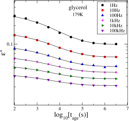
Figure 1: $\epsilon^{"}(t_{\mathrm{age}})$ data for glycerol at $179^{o}K$ vs. $t_{\mathrm{age}}$ (in sec) at the frequencies displayed in the inset. Solid lines correspond to the best fits using the modified KWW form with $\tau_{\mathrm{age}}(t_{\mathrm{age}})$ determined from eqn. (4).

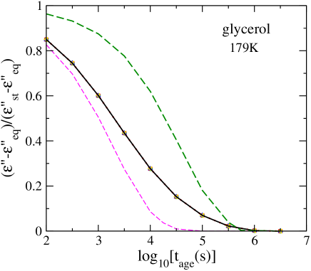
Figure 4: Scaling of the dielectric data for glycerol at $179^{o}K$ corresponding to different frequencies. Fits obtained with $\tau_{\mathrm{age}}(t_{\mathrm{age}})$ in the modified KWW ansatz determined from (a) Eqn. (4) of the present work (solid line) and (b) from Ref. lwsl (dashed line). Also shown are best fits obtained taking $\tau_{\mathrm{age}}$ = $\tau_{\mathrm{st}}$ (short dashed) and $\tau_{\mathrm{age}}$ = $\tau_{\mathrm{eq}}$ (long dashed) respectively with the stretching exponent being fixed at $\beta_{\alpha}$.

where the subscripts ”st” and ”eq” respectively refer to the initial ($t_{\mathrm{age}}\rightarrow 0$) and the long time ($t_{\mathrm{age}}\rightarrow\infty$) limiting values of $\epsilon^{"}$. In such a scheme generally both $\epsilon^{"}_{\mathrm{st}}$ and $\epsilon^{"}_{\mathrm{eq}}$ are obtained as the best value for the corresponding fitting parameters. The relaxation time $\tau_{\mathrm{age}}$ and stretching exponent $\beta_{\mathrm{age}}$ of the KWW form are also used as free fit parameters. The quality of this fitting with the dielectric data from different samples are available in Ref. lunken ( see fig. 1 and 2 there ). Both $\tau_{\mathrm{age}}$ and $\beta_{\mathrm{age}}$ as obtained from the fitting of the relaxation data in the aging regime show strong frequency dependence. If on the other hand we adopt a fitting scheme in which $\beta_{\mathrm{age}}$ is kept fixed at its corresponding $\alpha$-relaxation value $\beta_{\alpha}=.55$, then the data do not fit the form (1) with only $\tau_{\mathrm{age}}$ as a free fit parameter. The poorness of such a fitting procedure is discussed further below (see fig. 4).

An interesting interpretation of this data came from Lunkenheimer et. al. by using a modified KWW form with the relaxation time $\tau_{\mathrm{age}}$ being dependent on aging time $t_{\mathrm{age}}$ zotev ; tool . However in Ref. lwsl the time dependence of $\tau_{\mathrm{age}}$ is prescribed not in terms of the relaxation time but the corresponding frequency $\nu_{\mathrm{age}}$ which is defined as,

$$\nu(t_{\mathrm{age}})=\frac{1}{2\pi\tau_{\mathrm{age}}(t_{\mathrm{age}})}.$$ (2)

Lunkenheimer et. al. choose the aging time dependence of $\nu$ in (2) in the following form

$$\nu_{\mathrm{age}}\left(t_{\mathrm{age}}\right)=\left(\nu_{\mathrm{st}}-\nu_{\mathrm{eq}}\right)\exp\left[-{\left(2\pi\nu{t_{\mathrm{age}}}\right)}^{\beta_{\alpha}}\right]+\nu_{\mathrm{eq}}.$$ (3)

According to (3), the relaxation time $\tau_{\mathrm{age}}$ $\rightarrow$ $1/(2\pi\nu_{\mathrm{st}})$ and $1/(2\pi\nu_{\mathrm{eq}})$ as $t_{\mathrm{age}}$ $\rightarrow$ $0$ and $\infty$ respectively. Lunkenheimer et. al. obtain almost a perfect fit for the dielectric data over the whole frequency range with the above choice of the time dependence for the relaxation time. They observe that an important feature of this aging process is that the stretching exponent $\beta_{\mathrm{age}}$ is same as that of the $\alpha$-relaxation $\beta_{\alpha}$. It therefore implies that the stretching of the relaxation remains unaffected by aging below $T_{g}$ and hence conform to the validity of the time temperature superposition during the aging process. Furthermore the best fit value obtained for $\nu_{\mathrm{eq}}$ in (3) corresponds to a time $\tau_{\mathrm{eq}}=1/(2\pi\nu_{\mathrm{eq}})$ which agrees with the $\alpha$-relaxation time $\tau_{\alpha}$ for glycerol extrapolated from higher temperatures ( $T>T_{g}$ ) to sub-$T_{g}$ regions. This matching of $\tau_{\mathrm{eq}}$ with the extrapolated equilibrium $\alpha$-relaxation time values in case of glycerol will be further discussed below with fig. 5.

While this is a very instructive way of interpreting the evolution of the non equilibrium state, the anasatz (3) for determining the time evolution of $\tau_{\mathrm{age}}$ in terms of the corresponding frequency is somewhat unnatural. Instead of the relaxation time itself being time dependent, the corresponding frequency $\nu$ becomes time dependent in (3). The latter is then transmitted to $\tau_{\mathrm{age}}$ through the standard relation (2). As an alternative to this, in the present paper we adopt a more natural scheme for the time evolution of the relaxation time $\tau_{\mathrm{age}}$ in the following manner.

$$\tau_{\mathrm{age}}(t_{\mathrm{age}})=\left(\tau_{\mathrm{st}}-\tau_{\mathrm{fn}}\right)f(t_{\mathrm{age}})+\tau_{\mathrm{fn}}~{}~{}.$$ (4)

where the function $f(t)$ reduces to the value 1 or 0, for $t\rightarrow 0$ and $\infty$ respectively so that the relaxation time $\tau_{\mathrm{age}}$ attains the asymptotic values $\tau_{\mathrm{st}}$ and $\tau_{\mathrm{fn}}$ respectively in the above two limits. A perfect fit is obtained for all the $\epsilon^{"}(t_{\mathrm{age}})$ data at different frequencies using Eq. (1) with $\tau_{\mathrm{age}}(t_{\mathrm{age}})$ is being determined with the ansatz (4). In doing this the choice of the function $f(t)$ is not unique. However there are some characteristics that can be associated with this function. As indicated above it must change from $1$ to $0$ as the time changes from $t=0$ to $\infty$ limit. It is plausible to expect the time dependence of $f(t)$ is changing monotonically from 1 to 0. We have tested in terms of a reduced time $x=t/\tau$, where $\tau$ is the relaxation time the following three options: (a) exponential ( simple or stretched) relaxation like $\exp(-x^{\beta})$ (b) power law type decays $x^{-\alpha}$, or (c) a function which decays with the $\tanh(x)$. Among these the last form gives the best fit to the aging data. We obtain for the normalized function $f(t)$,

$$f(t)={{a_{o}}\over{{[1+\mathrm{e}^{2t/\tau(t)}]}^{\beta}}}$$ (5)

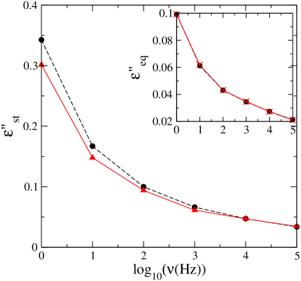
Figure 2: The best fit values of $\epsilon^{"}_{\mathrm{st}}$ for the curves in fig. 1 vs. frequency $\nu$(Hz) as obtained with the present work (solid line) and the corresponding results of Ref. lwsl (dashed). The inset shows the best fit $\epsilon^{"}_{\mathrm{eq}}$ with frequency $\nu$ respectively from the present work and Ref. lwsl .

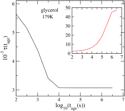
Figure 3: The best fit $\tau(t_{\mathrm{age}})$ vs. $t_{\mathrm{age}}$ (in sec) for glycerol using ansatz (4) of the present work. Result of Ref. lwsl for $\tau(t_{\mathrm{age}})$ as inset.

where $a_{o}=2^{1/\beta}$ is a normalization constant to ensure that $f(t)$ reduces to the above stated values in the two limits. Note that for times large compared to the relaxation times this function also behaves like a stretched exponential function with exponent $\beta$. Therefore the function defined in the self-consistent eqn. (5) also represents stretching of the relaxation process. The exponent $\beta$ for the stretching process is assumed to be same as the stretching exponent $\beta_{\mathrm{age}}$ used in the modified KWW form to keep the number of fitting parameters to a minimum. Thus in spite of the differences in the defining relations for the respective $\tau$’s, the $\beta_{\mathrm{age}}$ represents stretching of the relaxation process in both the cases (Ref.lwsl and ours). The fittings (corresponding to different $\omega$’s) over the whole frequency range of the dielectric data are shown in fig. 1. In the present fitting scheme unlike that of Ref. lwsl we obtain a stretching exponent $\beta_{\mathrm{age}}=.29$ which is different from the corresponding $\alpha$-relaxation value $\beta_{\alpha}=.55$. The best fit values for the parameters $\epsilon^{"}_{\mathrm{st}}$ and $\epsilon^{"}_{\mathrm{st}}$ ( at a given frequency ) obtained respectively in the present work and Ref. lwsl agree closely. This comparison is displayed in fig 2, We display next in fig. 3 the aging time dependence of $\tau_{\mathrm{age}}$ in our calculation and that of Ref. lwsl . In the present case the the relaxation time is strongly time dependent at the initial stage and saturates at relatively earlier as $t_{\mathrm{age}}$ reach the time $\tau_{\mathrm{fn}}$ (say). In our fitting scheme the best fit result value for $\tau_{fn}$ is very different from the corresponding $\tau_{\mathrm{eq}}$ of Lunkenheimer et. al. and cannot be simply related to the $\alpha$ relaxation process. All the dielectric data for $\epsilon^{"}$ scale into a single master curve as shown in the fig. 4. In the same figure we display the curve corresponding to the fitting of Lunkenheimer et. al. being practically indistinguishable from ours. We also display here for comparison the best fittings curves which are obtained with simple KWW function having constant relaxation times, respectively equal to $\tau_{\mathrm{st}}$ and $\tau_{\mathrm{eq}}$. The stretching parameter in both cases is $\beta_{\alpha}$. The inadequacy of a simple KWW form in fitting the observed data is clearly observable here.

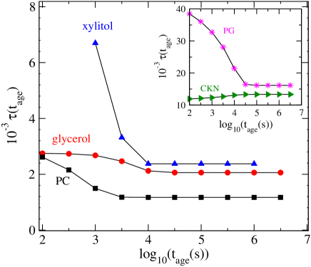
Figure 6: $\tau(t_{\mathrm{age}})$ vs. $t_{\mathrm{age}}$ (in sec) for different materials using ansatz (4) in the present work.

In addition to the dielectric data for glycerol, following Lunkenheimer et. al. we also fit using our scheme the dielectric data for Propylene carbonate ( PC, $T_{g}\approx 159\mathrm{K}$, $m=104$ ngai ), Propylene glycol( PG, $T_{g}\approx 168\mathrm{K}$, $m=52$ ngai ), xylitol ( $T_{g}\approx 248\mathrm{K}$, $m=94$ paluch ,paluch1 ) and structural relaxation for $\mathrm{[Ca(NO_{3})_{2}]_{0.4}[KNO_{3}]_{0.6}}$ ( CKN, $T_{g}\approx 333\mathrm{K}$, $m=93$ ) and the results are respectively shown in fig 5a-5d. The temperature ( below the corresponding $T_{g}$ ) in each case is also displayed in the figure. The variation of the relaxation time $\tau_{\mathrm{age}}(t_{\mathrm{age}})$ in the modified KWW form for fitting the data in each of the above materials is shown in fig 6. For all these materials, the general trend in aging time dependence of the relaxation time is the same as that in case of glycerol. $\tau_{\mathrm{age}}$ is strongly time dependent initially ( up to time $\tau_{\mathrm{fn}}$ ) and finally saturate to an almost constant value as is clearly visible in fig. 6. The TABLE I represents the stretching exponent $\beta_{\mathrm{age}}$ as a best fit parameter in the aging data for different materials obtained from present work (column 1) and also from Ref. lwsl (column 2).

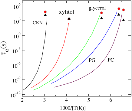
Figure 7: $\alpha$-relaxation time $\tau_{\alpha}$ vs. inverse of temperature for CKNloidl-de , xylitolluk , glycerowehn , PGngai1 , PCpimenov . The $\tau_{\mathrm{eq}}$ obtained from the fitting of the corresponding data is shown by filled circles for the fitting of Ref. lwsl and by filled triangles the present fitting scheme.

In case of the fitting scheme of Lunkenheimer et. al. the time scale $\tau_{\mathrm{eq}}$ agree with the extrapolated value of the $\alpha$-relaxation to the sub $T_{g}$ region. This is shown in fig. 7 for all the five materials whose relaxation data have been considered above. First $\tau_{\alpha}$’s for these materials with inverse temperature $1/T$ are shown. On the same figure we display for each curve ( with a filled circle ) the corresponding value of $\tau_{eq}=1/(2\pi\nu_{eq})$ obtained from the best fit value of (3) obtained by Lunkenheimer et. al. These points all lie on the corresponding extrapolated curve of the $\alpha$-relaxation times in the sub-$T_{g}$ regime. These authors conclude that the equilibrium $\alpha$-relaxation is determining the aging process . On the other hand the corresponding values of $\tau_{\mathrm{eq}}$ $\equiv$ $\tau_{\mathrm{fn}}$ obtained in our fitting scheme are shown for each curve with a filled triangle conforming to a relaxation mechanism of aging different from that of the equilibrium $\alpha$-relaxation.

We have presented here an alternative scenario for explaining the dielectric relaxation data of Lunkenheimer et. al. loidl-de in the aging regime. The present model proposes that the aging process involve two basic steps. In the first stage, the aging data fits to a modified stretched exponential form with a time dependent relaxation time $\tau_{\mathrm{age}}$. This is similar to the scheme of Lunkenheimer et. al. but the time dependence of $\tau_{\mathrm{age}}(t_{\mathrm{age}})$ is more natural here. As $t_{\mathrm{age}}$ reach a characteristic time scale $\tau_{\mathrm{fn}}$ the data can now be described in this second stage with a simple KWW form having a constant relaxation time comparable to $\tau_{\mathrm{fn}}$. This holds simultaneously for relaxation data at all frequencies as shown in fig 6. The limiting value of $\tau_{\mathrm{fn}}$ obtained here from fitting the data is however not same as that obtained from extrapolation of $\alpha$- relaxation times at higher temperatures to the sub-$T_{g}$ region. The stretching exponent $\beta_{\mathrm{age}}$ is also very different from that of the $\alpha$-relaxation process. The time dependence of the aging process and the corresponding relaxation time is possibly controlled by mechanisms which are different from that of equilibrium $\alpha$-relaxation.

The present analysis do not to claim in any way that the fitting scheme proposed by Lunkenheimer et. al. is invalid. The main difference of the model proposed here from that in ref. lwsl lies in the manner in which the relaxation time $\tau_{\mathrm{age}}$ depends on $t_{\mathrm{age}}$. In our scheme the relaxation time $\tau_{\mathrm{age}}$ is directly dependent on $t_{\mathrm{age}}$. This is distinct from adopting a some what unusual scheme of (3) in which the time dependence is imposed in the frequency $\nu_{\mathrm{age}}$. The justification of this scheme in which aging time dependence of $\tau_{\mathrm{age}}$ is defined in terms of the frequency is not obvious. The motivation for adopting such a scheme is that the asymptotic value for $\tau_{\mathrm{age}}$ (for long times) agrees with value of $\alpha$-relaxation times at higher temperatures extrapolated to the sub-$T_{g}$ region. There is no compelling reason to assume such a link between the non-equilibrium aging process and the equilibrium $\alpha$-relaxation.

To explain the last statement let us consider the correlation function $\mathcal{C}(t+t_{\mathrm{age}},t_{\mathrm{age}})$ of fluctuations at two different times $t_{\mathrm{age}}$ and $t+t_{\mathrm{age}}$. In the non-equilibrium state $\mathcal{C}$ depends on two times, i.e., both $t$ and $t_{\mathrm{age}}$. When time translational invariance holds, the dependence of $\mathcal{C}$ on $t_{\mathrm{age}}$ disappears. This happens over some time scale which is $\tau_{\mathrm{eq}}$. The correlation function now depends only on $t$ and the system has reached equilibrium. At this stage the relaxation is controlled by the $\alpha$-relaxation time $\tau_{\alpha}$. But the time scale $\tau_{\mathrm{eq}}$ which sets the dependence of the correlation function on $t_{\mathrm{age}}$ has no reason to be same as $\tau_{\alpha}$. In other words we insist that there is no aprirori reason to assume that the time evolution of $\epsilon^{"}$ during the aging process in the non equilibrium state is controlled by the equilibrium $\alpha$-relaxation process and the corresponding heterogeneity. Our work clearly shows here that the dielectric data can also be fitted with the modified KWW form with a different choice for the aging time dependence of the corresponding relaxation time.

An important aspect of the proposed relaxation behavior lies in the different time evolution of the relaxation time $\tau$ in comparison to that of Ref. lwsl . Here $\tau$ decreases with waiting time $t_{\mathrm{age}}$, implying that the aging process accelerates with time. It should however be noted that in the present case the relaxation time only decrease initially and then becomes almost constant. The stretching data at different frequencies correspond to a single relaxation time which is almost constant for aging time $t_{\mathrm{age}}$ beyond this initial scale $\tau_{\mathrm{fn}}$. The stretching exponent $\beta_{\mathrm{age}}$ for different frequency data is also the same. In Ref. lwsl the relaxation time $\tau$ actually grows with waiting time. Though somewhat speculative at this stage, such a difference in the basic nature of the aging process might imply a different microscopic mechanism for aging altogether. The more appropriate choice between the two schemes ( for fitting the aging data) discussed here can only be ascertained with a proper theoretical model for the evolution of the non equilibrium state.

SPD gratefully acknowledge A. Loidl and P. Lunkenheimer for providing the dielectric data and for the scientific discussions which stimulated the present work. We also acknowledge CSIR India for financial support.

	Stretching exponent $\beta_{\mathrm{age}}$
Materials	Present Work	Ref. lwsl
Glycerol	0.29	0.55 lwsl
PC	0.24	0.6 loidl-de ; luk
PG	0.23	0.58 wehn ; ngai1
xylitol	0.45	0.43 wehn
CKN	0.34	0.4 pimenov

Table 1: The stretching exponent $\beta_{\mathrm{age}}$ as a best fit parameter in the aging data for different materials obtained (a) from present work (column 1) (b) from Ref. lwsl (column 2). The corresponding reference from which the data for $\alpha$-relaxation is taken are also provided in col. 2

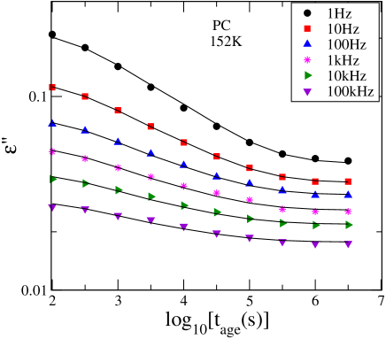
Figure 5a: $\epsilon^{"}(t_{\mathrm{age}})$ data for PC loidl-de ; luk at $152^{o}K$ vs. $t_{\mathrm{age}}$ (in sec) at the frequencies displayed in the inset. The solid lines are obtained using our scheme.

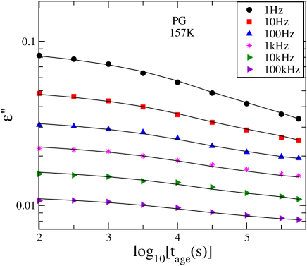
Figure 5b: $\epsilon^{"}(t_{\mathrm{age}})$ data for PG wehn ; ngai at $157^{o}K$ vs. $t_{\mathrm{age}}$ (in sec) at the frequencies displayed in the inset. The solid lines are obtained using our scheme.

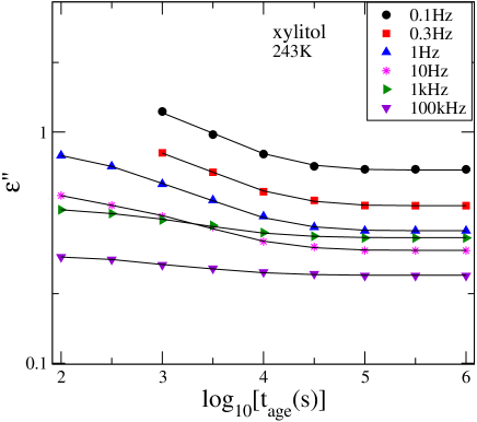
Figure 5c: $\epsilon^{"}(t_{\mathrm{age}})$ data for xylitol wehn at $243^{o}K$ vs. $t_{\mathrm{age}}$ (in sec) at the frequencies displayed in the inset. The solid lines are obtained using our scheme.

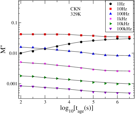
Figure 5d: $M^{"}(t_{\mathrm{age}})$ data for CKN pimenov at $329^{o}K$ vs. $t_{\mathrm{age}}$ (in sec) at the frequencies displayed in the inset. The solid lines are obtained using our scheme.

References

- (1) M.D. Ediger, C.A. Angell, and S.R. Nagel, J. Phys. Chem. 100, 13200(1996); C.A. Angell et al., J. Appl. Phys. 88, 3113 (2000)
- (2) L.C.E. Struik, Physical Aging In Amorphous Polymers and Other Materials (Elsevier, Amsterdam, 1978)
- (3) W. Kob and J. L. Barrat, Phys. Rev. Lett. 38, 4581 (1997).
- (4) L.F. Cugliandolo and J. Kurchan, Phys. Rev. Lett. 71, 173 (1993).
- (5) P. Lunkenheimer, R. Wehn, U. Schneider, and A. Loidl, Phys. Rev. Lett. 95, 055702 (2005).
- (6) U. Schneider, R. Brand, P. Lunkenheimer, and A. Loidl, Phys. Rev. Lett. 84, 5560 (2000).
- (7) C.A. Angell, in Relaxations in Complex Systems, edited by K.L. Ngai and G.B. Wright (NRL, Washington, DC,1985), p. 3.
- (8) R. Böhmer, K.L. Ngai, C.A. Angell, and D.J. Plazek, J.Chem. Phys. 99, 4201 (1993)
- (9) R. L. Leheny and S. R. Nagel, Phys. Rev. B 57, 5154 (1998).
- (10) P. Lunkenheimer, R. Wehn, A. Loidl, J. Non-Cryst. Solids 352 4941(2006)
- (11) V. S. Zotev, G. F. Rodriguez, G. G. Kenning, R. Orbach, E. Vincent and J. Hammann, Phys. Rev. B 67, 184422 (2003)
- (12) A.Q. Tool, J.Am. Ceram. Soc. 29, 240 (1946); O.S. Narayanaswamy, ibid. 54, 240 (1971).
- (13) A. Döß, M. Paluch, H. Sillescu, and G. Hinze, Phys. Rev. Lett. 88, 095701 (2002).
- (14) A. Döß, M. Paluch, H. Sillescu, and G. Hinze, J. Chem. Phys. 117, 6582 (2002); A. Minuguchi, K. Kitai, and R. Nozaki, Phys. Rev. E 68, 031501 (2003).
- (15) P. Lunkenheimer, U. Schneider, R. Brand, and A. Loidl, Contemp. Phys. 41 15 (2000).
- (16) R. Wehn et al. (to be published).
- (17) K. L. Ngai et al., J. Chem. Phys. 115, 1405 (2001).
- (18) A. Pimenov, P. Lunkenheimer, H. Rall, R. Kohlhaas, A. Loidl and R Böhmer, Phys. Rev. E 54, 676 (1996).