A Fast Hierarchical Multilevel Image Segmentation Method using Unbiased Estimators

Abstract

This paper proposes a novel method for segmentation of images by hierarchical multilevel thresholding. The method is global, agglomerative in nature and disregards pixel locations. It involves the optimization of the ratio of the unbiased estimators of within class to between class variances. We obtain a recursive relation at each step for the variances which expedites the process. The efficacy of the method is shown in a comparison with some well-known methods.

I Introduction

Thresholding is an important technique for image segmentation and object extraction. The aim of an effective segmentation is to separate objects from the background and to differentiate pixels having nearby values for improving the contrast. The use of binary images reduces the computational cost of the succeeding steps and increases the ease of manipulation compared to using gray-level images. Image thresholding is a well-researched field and there exist many algorithms for determining an optimal threshold of the image. Many surveys of thresholding methods and their applications exist in literature [1], [2].

Thresholding techniques can be divided into bilevel and multilevel categories, depending on the number of classes. In bilevel thresholding, the image is segmented into two different regions. The pixels with gray-level values greater than a certain value T are classified as object pixels, and the others with values lesser than T are classified as background pixels or vice versa. Otsu’s method [4] chooses optimal thresholds by maximizing the between class variance and minimizing within class variance. Sahoo et al. [10] found that in global thresholding, Otsu’s method is one of the better threshold selection methods for general real world images with regard to uniformity and shape measures. However, inefficient formulation of between class variance makes the method time consuming. Abutaleb [5] used two-dimensional entropy to calculate the threshold. Kittler and Illingworth [12] suggested a minimum error thresholding method. They assume that an image is characterized by a mixture distribution with both object and background classes having a Gaussian distribution. The probability density function for each class is estimated based on the histogram of the image. Kwon [6] proposed a threshold selection method based on cluster analysis. The method proposed a criterion function that involved not only the histogram of the image but also the information on spatial distribution of pixels. This criterion function optimizes intra-class similarity to achieve the most similar class and inter-class similarity to confirm that every cluster is well separated. The similarity function uses all pixels in the two clusters as denoted by their coordinates.

Multilevel thresholding is a process that segments a gray-level image into several distinct regions. The method works very well for objects with colored or complex backgrounds, on which bilevel thresholding fails to produce satisfactory results. Reddi et al. [7] proposed an iterative form of Otsu’s method, so as to generalize it to multilevel thresholding. Ridler and Calward algorithm [8] uses an iterative clustering approach. An initial estimate of the threshold is made (e.g., mean image intensity) and pixels above and below are assigned to the white and black classes respectively. The threshold is then iteratively re-estimated as the mean of two class means. The most difficult task is to determine the appropriate number of thresholds automatically. Papamarkos and Gatos [13] specify the multithreshold values as the global minima of the rational functions which approximate the histogram segments by using hill clustering technique to determine the peak locations of image histogram. Arora et al. [9] propose a simple multilevel thresholding using means and variances. Here we also point out that the extension of various binarization methods become extremely complex for multilevel segmentation due to the curse of dimensionality. We will discuss this with respect to Otsu’s method. Arifin and Asano [11] propose a hierarchical clustering method, which is shown to be more efficient than some existing methods. In their method, they use agglomerative clustering (using a dendrogram of gray levels) based on a similarity measure which involves the interclass variance of the clusters to be merged and the intra-class variance of the newly merged cluster.

We use unbiased estimators of variances for optimization and find a recursive formulation which improves computational efficiency of the algorithm. We then compare our results with these well known global thresholding methods and find that the proposed approach is better than most existing techniques on the criteria that we consider.

II Approach and Algorithm

In the proposed approach, we will optimize the ratio of unbiased estimators of within and between class variances of the image to find thresholds for segmenting the image into multiple levels. The method is agglomerative hierarchical where we merge two classes at each level, and replace the pixels belonging to either class by their weighted mean gray-level. Thus we reduce the number of classes by one at each iteration. This procedure can be easily imagined in terms of a dendrogram. A similar approach has been used for petrophysical data classification in [14] and by Acharya et al. in [15]. Let $G$ be the number of levels of the gray scale image, so that the number of classes initially is $G$. Also let $M$ be the a priori known desired number of classes. Let $t_{i}$ be the $i^{th}$ threshold at a given stage and $C_{k}$ be the $k^{th}$ class, defined as $\{\hskip 2.84526ptg\mid t_{k-1}<g\leq t_{k}\}$, where $g$ denotes a gray-level between $1$ and $G$. The thresholds $t_{0}$ and $t_{M}$ are defined to be 0 and $G$, respectively.

A histogram $h(g)$ is the function which shows the number of occurrences of the gray-level $g$ in the image. If $N$ is the total number of pixels in the image then, $N$ = $\sum_{g=1}^{G}h(g)$

$K(i)$ = the number of classes after the $i^{th}$ recursion of the algorithm. Thus $K(0)=G$.

$n_{k}(i)$ = the number of pixels in the $k^{th}$ class after the $i^{th}$ recursion

$a_{k}(i)$ = the amplitude of the $k^{th}$ class after $i^{th}$ recursion,

$a$ = the grand weighted mean gray-level of all the pixels in the image. Note that $a_{k}(i)$ refers to the weighted pixel value (or gray-level) of the pixels in class $C_{k}(i)$, i.e., class $C_{k}$ at the $i^{th}$ recursion.

$x_{km}(i)$ = the $m^{th}$ pixel in the $k^{th}$ class after the $i^{th}$ recursion. Note that wherever $i$ is not defined, it refers to the recursion number.

We define the unbiased estimator of within-class variance $v(i)$ and that of between-class variance $w(i)$ at the $i^{th}$ recursion by the following equations:

$$v(i)=\frac{1}{N-K(i)}\sum_{k=1}^{K(i)}\sum_{m=1}^{n_{k}(i)}[x_{km}(i)-a_{k}(i)]^{2}$$ (1)

$$w(i)=\frac{1}{K(i)-1}\sum_{k=1}^{K(i)}n_{k}(i)[a_{k}(i)-a]^{2}$$ (2)

The criterion function is given by $q(i)$

$$q(i)=\frac{v(i)}{w(i)}$$ (3)

where $q(i)$ is the value of the function to be minimized after the $i^{th}$ iteration.

An exhaustive search which calculates the objective function for every pair of connected classes eligible to be merged is computationally cumbersome. We derive a recursive formulation which avoids this. Suppose we are in the $(i-1)^{th}$ stage and the pair of classes to be combined are $C_{l}(i-1)$ and $C_{l+1}(i-1)$. From equation 1, we have

$$v(i-1) = \frac{1}{N-K(i-1)}\sum_{k=1}^{K(i-1)}\sum_{m=1}^{n_{k}(i-1)}[x_{km}(i-1)-a_{k}(i-1)]^{2}$$

$$= \frac{1}{N-K(i-1)}\Big{\{}\sum_{k=1,k\neq l,l+1}^{K(i-1)}\Big{(}\sum_{m=1}^{n_{k}(i-1)}[x_{km}(i-1)-a_{k}(i-1)]^{2}\Big{)}$$

$$+\sum_{m=1}^{n_{l}(i-1)}[x_{lm}(i-1)-a_{l}(i-1)]^{2}$$

$$+\sum_{m=1}^{n_{l+1}(i-1)}[x_{l+1,m}(i-1)-a_{l+1}(i-1)]^{2}\Big{\}}$$

After $C_{l}(i-1)$ and $C_{l+1}(i-1)$ are merged, the number of classes will be reduced by one ($K(i)=K(i-1)-1$) and the last two terms above will be changed. Writing $v(i)$ in terms of the parameters in the $(i-1)^{th}$ recursion, we get

$$v(i) = \frac{1}{N-K(i-1)+1}\Big{\{}\sum_{k=1,k\neq l,l+1}^{K(i-1)}\Big{(}\sum_{m=1}^{n_{k}(i-1)}[x_{km}(i-1)-a_{k}(i-1)]^{2}\Big{)}$$

$$+\sum_{m=1}^{n_{l}(i-1)}[x_{lm}(i-1)-a_{l^{\prime}}(i)]^{2}+\sum_{m=1}^{n_{l+1}(i-1)}[x_{l+1,m}(i-1)-a_{l^{\prime}}(i)]^{2}\Big{\}}$$

where,

$$a_{l^{\prime}}(i)=\frac{n_{l}(i-1)a_{l}(i-1)+n_{l+1}(i-1)a_{l+1}(i-1)}{n_{l}(i-1)+n_{l+1}(i-1)}$$ (4)

is the combined mean gray-level of the classes $C_{l}(i-1)$ and $C_{l+1}(i-1)$ after they merge.

Comparing the above few equations, and doing some algebraic manipulations, we ultimately get

$$v(i)=\frac{N-K(i-1)}{N-K(i)}\hskip 2.84526ptv(i-1)+\frac{1}{N-K(i)}\hskip 2.84526ptd_{l}(i-1)^{2}$$ (5)

where

$$d_{l}(i-1)^{2}=\frac{n_{l}(i-1)n_{l+1}(i-1)}{n_{l}(i-1)+n_{l+1}(i-1)}\hskip 2.84526pt[a_{l}(i-1)-a_{l+1}(i-1)]^{2}$$ (6)

Similarly, we obtain

$$w(i)=\frac{K(i-1)-1}{K(i)-1}\hskip 2.84526ptw(i-1)-\frac{1}{K(i)-1}\hskip 2.84526ptd_{l}(i-1)^{2}$$ (7)

The equations 5, 7 give a recursive formulation to calculate the within and between class variances. We see that the only term controlling the increment of $v(i)$ and the decrement of $w(i)$ is the term $d_{l}(i-1)^{2}$, and thus minimizing $d_{l}(i-1)^{2}$ helps us in optimizing $q(i)$.

II-A Algorithmic Implementation

As above, let $M$ be the number of classes desired after segmentation. The stepwise implementation of the above algorithm is given below:

• Initialize the number of classes by the number of gray-levels ($K(0)=G$).

• Calculate $d_{k}^{2}$ for all pairs of adjacent classes for the $0^{th}$ stage.

• For each stage $i\leftarrow i+1$, until $K(i)\geq M$, Do:

1. Combine the $l^{th}$ and $(l+1)^{th}$ segments, where $l$ is the index for which $d_{l}^{2}$ yields its minimum value.

2. Update the necessary as follows:

   $$K(i) = K(i-1)-1$$

   $$a_{l}(i) = \frac{n_{l}(i-1)a_{l}(i-1)+n_{l+1}(i-1)a_{l+1}(i-1)}{n_{l}(i-1)+n_{l+1}(i-1)}$$

   $$n_{l}(i) = n_{l}(i-1)+n_{l+1}(i-1)$$

   $$a_{l-m}(i) = a_{l-m}(i-1);\hskip 80.94205ptm=1,2,\ldots l-1$$

   $$a_{l+m}(i) = a_{l+m+1}(i-1);\hskip 72.26999ptm=1,2,\ldots K(i)-l$$

   $$n_{l-m}(i) = n_{l-m}(i-1);\hskip 80.94205ptm=1,2,\ldots l-1$$

   $$n_{l+m}(i) = n_{l+m+1}(i-1);\hskip 72.26999ptm=1,2,\ldots K(i)-l$$

   $$d_{l-1}(i)^{2} = \frac{n_{l-1}(i)n_{l}(i)}{n_{l-1}(i)+n_{l}(i)}\hskip 2.84526pt[a_{l-1}(i)-a_{l}(i)]^{2}$$

   $$d_{l}(i)^{2} = \frac{n_{l}(i)n_{l+1}(i)}{n_{l}(i)+n_{l+1}(i)}\hskip 2.84526pt[a_{l}(i)-a_{l+1}(i)]^{2}$$

   $$d_{l-1-m}(i)^{2} = d_{l-1-m}(i-1)^{2};\hskip 72.26999ptm=1,2,\ldots l-2$$

   $$d_{l+m}(i)^{2} = d_{l+1+m}(i-1)^{2};\hskip 72.26999ptm=1,2,\ldots K(i)-l-1$$

3. The cumulative sums of the $n_{k}$’s yield us the values of thresholds.

III Multilevel thresholding and Computational Advantage over Otsu

The algorithm proposed can be used for multilevel image thresholding as well as binarization. For having a particular number of classes, we have to stop at a stage when the number of levels equals the number of classes desired. This method has the advantage of being computationally much more efficient than Otsu’s, in spite of having a very similar criterion function. We also know that of all methods possible, Otsu’s technique will have the minimum Peak-Signal-to-Noise-Ratio (PSNR) value because PSNR acts like the criterion function for Otsu’s algorithm. We theoretically evaluate the performance of the proposed algorithm and compare it with conventional Otsu’s method for multilevel thresholding. For segmenting an image with $G$ gray-levels using $n$ thresholds, Otsu’s exhaustive search method searches $G\choose n$ different combinations of thresholds, which can be approximated to $G^{n}$ for $n<<G$. Thus the time complexity is exponential in the number of thresholds.

Claim: The proposed method can calculate all the possible thresholds in the multilevel case in $O(G^{2})$ time.

Proof: We can divide the algorithm into three parts:

1. Finding the minima of $d_{l}^{2}$, which takes $O(K(i))$ steps for the $i^{th}$ iteration.

2. Updating the parameters, which can be done in $O(1)$ time.

3. Writing down the thresholds will take at most $O(K(i))$ time. We can also store the values efficiently by storing only the classes being merged at each stage.

Thus, if we run the entire algorithm until we are left with two classes ($G-1$ iterations), it will take $O(G^{2})$ time, thus providing a tremendous edge in terms of computational time over the exponentially complex Otsu’s thresholding. We also point out here that most of the hierarchical thresholding algorithms (for example [11]) will also consume $O(G^{2})$ time, but the proposed method, because of its unique recursive formulation, incurs low costs even in terms of the actual number of computations.

IV Results and Observations

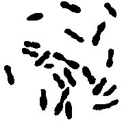
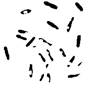
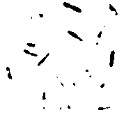
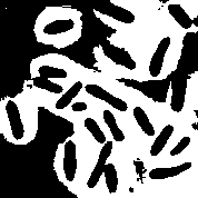
For evaluating the performance of the proposed algorithm, we have implemented the method on a wide variety of images for both binarization and multilevel thresholding. The image set we used for comparing the performance of our algorithm with other methods for the bilevel case is shown in Fig. 1. Along with the results obtained using the proposed technique, those of four other methods have been shown - Otsu’s [4], Kwon’s [6], Kittler-Illingworth’s [12] and Arifin-Asano’s [11].

(a) Bacteria

(b) Coins

(c) Fish

(d) Things

(e) Rice

Figure 1: Various Images we use for comparison.

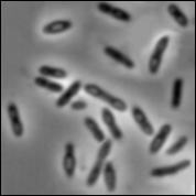
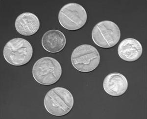
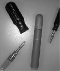
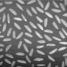
The results are compared with the ground truth images generated by manual thresholding (See Figs. 2, 3, 4, 5, 6) We observe that our method works at least at par with the other methods, and in most of the cases produces a superior classification.

In order to compare the quality of the thresholded images quantitatively, we have evaluated the performance of the proposed method against the four different methods, using the criteria of misclassification error (ME) and relative foreground area error (RAE) [2].

ME is defined in terms of the correlation of the images with human observation. It corresponds to the ratio of background pixels wrongly assigned to foreground, and vice versa. ME can be simply expressed as:

$$ME=1-\frac{|B_{O}\bigcap B_{T}|+|F_{O}\bigcap F_{T}|}{B_{O}+F_{O}}$$ (8)

where background and foreground are denoted by $B_{O}$ and $F_{O}$ for the original image (the ground truth image), and by $B_{T}$ and $F_{T}$ for the test image, respectively.

RAE measures the number of discrepancies in the thresholded image with respect to the reference image, taking the area of the foreground into account. It is defined as

$$RAE=\left\{\begin{array}[]{cl}\frac{A_{O}-A_{T}}{A_{O}},&A_{O}>A_{T}\\ \frac{A_{T}-A_{O}}{A_{T}},&A_{T}\geq A_{O}\end{array}\right.$$ (9)

where $A_{O}$ is the area of the reference image, and $A_{T}$ is the area of thresholded image.

(a) Ground

(b) Arifin

(c) Otsu

(d) KI

(e) Kwon

(f) Proposed

Figure 2: Bacteria Image results for various methods

(a) Ground

(b) Arifin

(c) Otsu

(d) KI

(e) Kwon

(f) Proposed

Figure 3: Coins Image results for various methods

(a) Ground

(b) Arifin

(c) Otsu

(d) KI

(e) Kwon

(f) Proposed

Figure 4: Rice Image results for various methods

(a) Ground

(b) Arifin

(c) Otsu

(d) KI

(e) Kwon

(f) Proposed

Figure 5: Fish Image results for various methods

(a) Ground

(b) Arifin

(c) Otsu

(d) KI

(e) Kwon

(f) Proposed

Figure 6: Things Image results for various methods

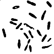
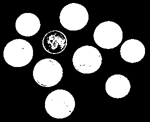
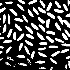
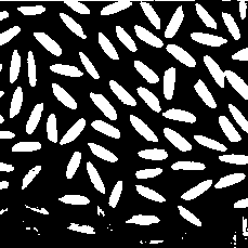
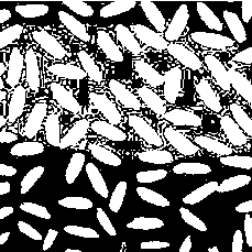
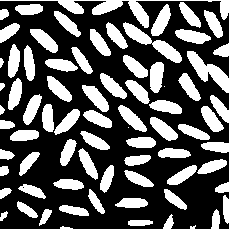
In Table I we show the ME and RAE for the various images under consideration.

Image	Arifin	Otsu	KI	Kwon	Proposed
$ME$
Bacteria	0.0857	0.0432	0.1253	0.3316	0.0459
Rice	0.0589	0.0741	0.0924	0.1719	0.0609
Fish	0.1745	0.0673	0.0356	0.2860	0.0263
Coins	0.0163	0.0135	0.0076	0.1887	0.0066
Things	0.1759	0.0432	0.1772	0.2669	0.0515
$RAE$
Bacteria	0.4629	0.1893	0.7027	0.6394	0.2200
Rice	0.0318	0.1495	0.2311	0.2973	0.0325
Fish	0.7981	0.2929	0.1276	0.5675	0.0859
Coins	0.0514	0.0426	0.0200	0.3726	0.0095
Things	0.1912	0.0448	0.1923	0.3356	0.0204

TABLE I: Comparison of ME and RAE for various images on the methods

In this section, we also consider another measure called the Peak Signal-to-Noise Ratio (PSNR) of the segmented image. Let $S$ be the source image and $T$ be the image obtained after thresholding ($S$ means $S(i,j)$ and $T$ means $T(i,j)$). $N$ is the total number of pixels in the image. Let us assume for the time being that the number of gray-levels is 256. Then, the mean square error (MSE) and the PSNR are given by:

$$MSE = \frac{\sum{[S-T]^{2}}}{N}$$ (10)

$$PSNR = 10\log_{10}{\left(\frac{255^{2}}{MSE}\right)},$$ (11)

where the summation in MSE is over all the pixels in the image and the PSNR value obtained above is in dB (decibels).

PSNR is used to determine the overall quality and error of thresholded image. Several test images were taken and PSNR was calculated for thresholded images for multiple levels using the proposed technique. The results are shown in Table II. We can see that the value of PSNR grows in general with the number of classes, and this combined with the computational advantage discussed above makes the process valuable. The table of PSNR values gives us an idea that the method can be used for “fast” lossy compression in real time in a general setting owing to high PSNR values. We give examples of natural and smooth pictures in addition to the images considered above because the objective here is compression and not object recognition.

Image	2 level	3 level	5 level	10 level	25 level
Lena	20.3	23.6	27.0	33.4	41.1
Baboon	20.1	24.1	27.8	32.8	40.6
Peppers	19.2	21.6	26.4	32.1	39.8
Rice	21.4	23.6	28.5	34.1	41.8
Fish	21.3	26.6	30.8	36.2	43.4
Things	18.7	21.2	26.7	31.6	39.5

TABLE II: PSNR Values for various levels of image thresholding by proposed method

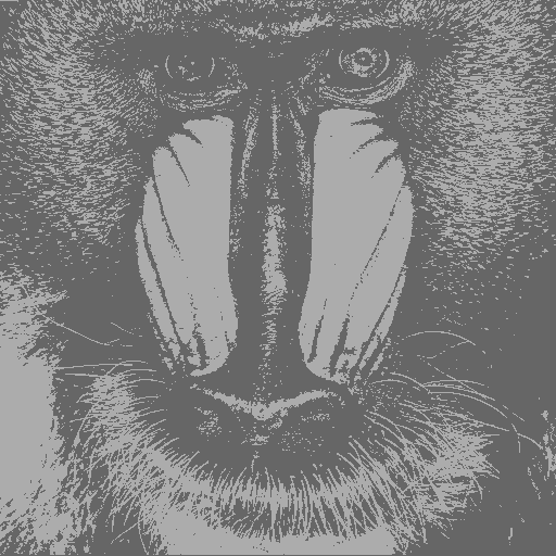
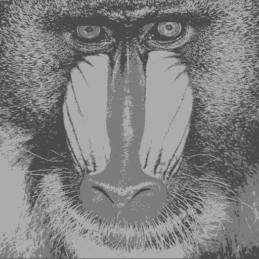
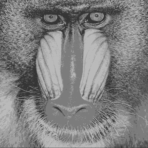
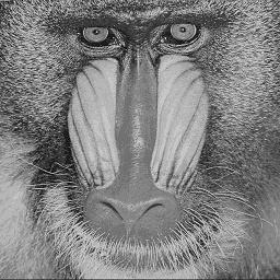
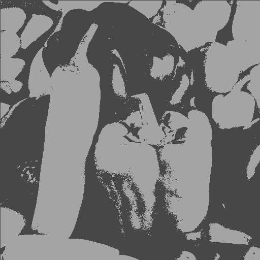
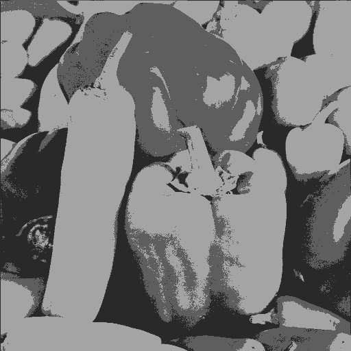
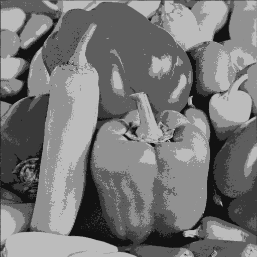
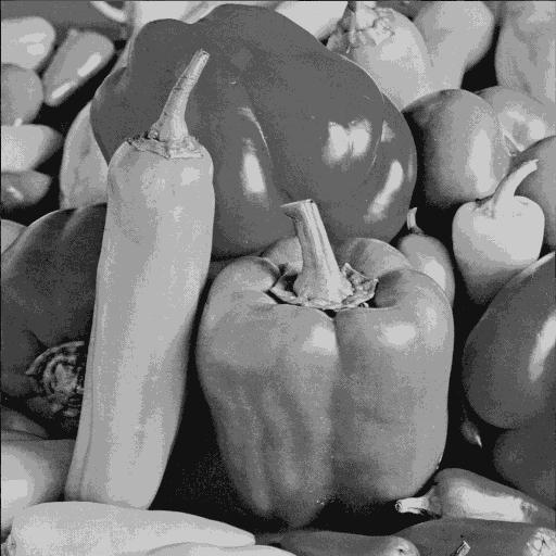
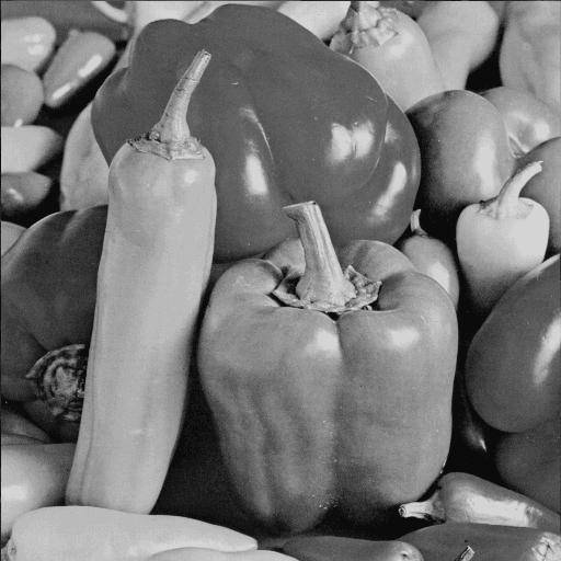
We show the original and thresholded images for some well known images in Figs. 7, 8, 9 obtained using the proposed method. Note that for the bilevel case, we show images with gray-levels equal to the means of the two classes.

(a) Gray

(b) 2 Level

(c) 3 Level

(d) 5 Level

(e) 10 Level

(f) 25 Level

Figure 7: Lena image thresholding Image results for various levels.

(a) Gray

(b) 2 Level

(c) 3 Level

(d) 5 Level

(e) 10 Level

(f) 25 Level

Figure 8: Baboon image thresholding Image results for various levels.

(a) Gray

(b) 2 Level

(c) 3 Level

(d) 5 Level

(e) 10 Level

(f) 25 Level

Figure 9: Peppers image thresholding Image results for various levels.

V Conclusion

We have proposed a novel image segmentation technique based on unbiased variance estimators. The proposed method is compared with other global histogram-based thresholding methods. The various results show the efficiency of the proposed method with respect to object recognition and also for compression owing to a high PSNR associated with it. The method is also computationally very advantageous because of its polynomial running time.

References

- [1] Z. Chi, H. Yan, T. Pham, “Fuzzy Algorithms: With applications to images processing and pattern recognition,” World Scientific, Singapore, 1996..
- [2] M. Sezgin and B. Sankur, “Survey over image thresholding techniques and quantitative performance evaluation”, Journal of Electronic Imaging, 13(1), 146-165, 2004.
- [3] W. Niblack, “An Introduction to Digital Image Processing,” Englewood Cliffs, N. J.: Prentice Hall, 115-116, 1986.
- [4] N. Otsu, “A threshold selection using gray level histograms,” IEEE Trans. Systems Man Cybernetics, 9, 62-69, 1979.
- [5] A. S. Abutaleb, “Automatic thresholding of gray level pictures using two-dimensional entropy,” Comput. Vision Graphics Image Process. 47, 22-32, 1989.
- [6] S. H. Kwon, “Threshold selection based on cluster analysis,” Pattern Recognition Letters, 25, 1045 1050, 2004.
- [7] S. S. Reddi, S. F. Rudin, H. R. Keshavan, “An Optical Multiple Threshold Scheme for Image Segmentation”, IEEE Trans. System Man and Cybernetics, 14, 661-665, 1984.
- [8] T. W. Ridler, S. Calward, “Picture Thresholding Using an Iterative Selection Method”, IEEE Trans. Systems, Man and Cybernetics, 8, 630-632, 1978.
- [9] S. Arora, J. Acharya, A. Verma, P. K. Panigrahi, “Multilevel Thresholding for Image Segmentation through a Fast Statistical Recursive Algorithm,” Pattern Recognition Letters, 29, 119 125, 2008.
- [10] P. K. Sahoo, S. Soltani, A. K. C. Wong, “SURVEY: A survey of thresholding techniques”, Comput. Vision Graphics Image Process, 41, 233-260, 1988.
- [11] A. Z. Arifin, A. Asano, “Image segmentation by histogram thresholding using hierarchical cluster analysis,” Pattern Recognition Letters, 27, 1515-1521, 2006.
- [12] J. Kittler, J. Illingworth, “Minimum error thresholding,” Pattern Recognition, 19(1), 41-47, 1986.
- [13] N. Papamarkos, B. Gatos, “A new approach for multilevel threshold selection,” Graphics Models Image Process, 56, 357-370, 1996.
- [14] A. Moghaddamjoo, “Optimum Well-Log Signal Segmentation,”IEEE Transactions on Geoscience and Remote Sensing, 27(5), 633 - 641, 1989.
- [15] J. Acharya, G. Sreechakra, J. C. Goswami, D. Heliot, “Hierarchical Zonation Technique to Extract Common Boundaries of a Layered Earth Model,” Proceedings of the IEEE Antenna and Propagation Society Symposium, Hawaii, 2007.