Asymptotic Mutual Information Statistics of Separately-Correlated Rician Fading MIMO Channels

Giorgio Taricco
(19 December 2007)
Abstract

Precise characterization of the mutual information of MIMO systems is required to assess the throughput of wireless communication channels in the presence of Rician fading and spatial correlation. Here, we present an asymptotic approach allowing to approximate the distribution of the mutual information as a Gaussian distribution in order to provide both the average achievable rate and the outage probability. More precisely, the mean and variance of the mutual information of the separately-correlated Rician fading MIMO channel are derived when the number of transmit and receive antennas grows asymptotically large and their ratio approaches a finite constant. The derivation is based on the replica method, an asymptotic technique widely used in theoretical physics and, more recently, in the performance analysis of communication (CDMA and MIMO) systems. The replica method allows to analyze very difficult system cases in a comparatively simple way though some authors pointed out that its assumptions are not always rigorous. Being aware of this, we underline the key assumptions made in this setting, quite similar to the assumptions made in the technical literature using the replica method in their asymptotic analyses. As far as concerns the convergence of the mutual information to the Gaussian distribution, it is shown that it holds under some mild technical conditions, which are tantamount to assuming that the spatial correlation structure has no asymptotically dominant eigenmodes. The accuracy of the asymptotic approach is assessed by providing a sizeable number of numerical results. It is shown that the approximation is very accurate in a wide variety of system settings even when the number of transmit and receive antennas is as small as a few units.

$*$$*$footnotetext: This work is supported by the STREP project No. IST-026905 (MASCOT) within the sixth framework programme of the European Commission. These results have been presented in part at the IEEE GLOBECOM 2006, Communication Theory Symposium.

I Introduction

During the last decade, multiple-input multiple-output (MIMO) wireless systems attracted much interest because of the prediction of outstanding capacity gains with respect to corresponding single-input single-output (SISO) systems [50, 11, 46].

Early work in this area was mostly based on the assumption of independent and identical distributed (iid) Rayleigh fading paths justified by the rich scattering assumption [11].

However, experimental and theoretical results showed that more realistic MIMO channel models are required to obtain more accurate results, which can dramatically impact the potential capacity gains [12, 13, 42]. Thus, more realistic channel models have been proposed in the literature accounting for both multipath correlation and the presence of a line-of-sight (LOS) component (Rician fading).

In this work we focus on the separately-correlated MIMO Rician fading channel whose channel matrix can be written as

𝐇=𝐇¯+𝐑1/2𝐇w𝐓1/2,𝐇¯𝐇superscript𝐑12subscript𝐇𝑤superscript𝐓12\mathbf{H}=\bar{\mathbf{H}}+\mathbf{R}^{1/2}\mathbf{H}_{w}\mathbf{T}^{1/2},

where 𝐇¯¯𝐇\bar{\mathbf{H}} is a constant matrix accounting for the LOS component, 𝐑,𝐓𝐑𝐓\mathbf{R},\mathbf{T} are the nonnegative definite receive and transmit correlation matrices, respectively, and 𝐇wsubscript𝐇𝑤\mathbf{H}_{w} is a matrix of iid circularly-symmetric zero-mean complex Gaussian random variables. We assume that the channel parameters (𝐇¯,𝐑,𝐓)¯𝐇𝐑𝐓(\bar{\mathbf{H}},\mathbf{R},\mathbf{T}) are unknown at the transmitter whereas the receiver knows the channel matrix realization exactly (i.e., following the terminology introduced by Goldsmith et al. [13], there is perfect channel-state information at the receiver (CSIR) and no channel distribution information at the transmitter (CDIT)).

In the MIMO Rician fading channel literature, many works focus on the spatially uncorrelated channel. In particular, Hösli et al. [19] show that the mutual information is monotonically non-decreasing in the singular values of 𝐇¯¯𝐇\bar{\mathbf{H}}. Jayaweera and Poor [22] derive the exact ergodic capacity when only the Rice factor K𝐾K known at the transmitter by using the joint eigenvalue distribution of the noncentral Wishart matrix, and lower and upper bounds to the ergodic capacity when full CDIT is available. Hansen and Bölcskei [18] investigate the case of high SNR with unit–rank average channel matrix. Venkatesan et al.[47] derive the capacity-achieving covariance matrix of the channel, generalizing previous results relevant to the case of unit rank 𝐇¯¯𝐇\bar{\mathbf{H}} [21]. Kang and Alouini [25] obtain the exact ergodic capacity by calculating the determinant of a matrix whose entries contain confluent hypergeometric functions of the second kind and the exact capacity variance in terms of Meijer s G-functions.

Many recent works propose upper and lower bounds to the capacity of the separately correlated Rician fading MIMO channel. McKay and Collings [31, 32] derive upper and lower bounds to the ergodic mutual information, based on the method of zonal polynomials, which are asymptotically tight as the SNR grows to infinity. They also provide an asymptotic (in the SNR) expression of the mutual information variance. The bounds have been further refined in [33]. In the same context, Cui et al. [3] obtain similar upper and lower bounds to the ergodic capacity by using a determinant expansion in terms of minors whose moments are calculated by use of hypergeometric matrix functions. In a recent paper, Lebrun et al.[28] use asymptotic bounds to confirm that the mean and variance of the MIMO channel capacity approach the values of the corresponding underlying scattering channel when the number of antennas is large and the average channel matrix has unit rank.

Another way to circumvent the difficulties related to the derivation of an exact expression of the capacity consists of assuming an asymptotically large number of transmit and receive antennas.

In this contest, Moustakas et al. [34] show that the capacity of the correlated Rayleigh fading MIMO channel converges to a Gaussian random variables whose mean and variance are calculated in closed form. Their derivation is based on approximating the moment generating function (MGF) of the capacity by using the replica method, a technique originally introduced in the context of statistical physics and successfully applied to several communications problems (see, e.g., [37, 14, 43, 49]).

A considerable number of research works in this area are based on the use of Stieltjes Transform and lead to results compatible to those presented here. Among them, Dumont et al. [5] derived the asymptotic mutual information mean in the case of single-sided (receiver side) separately-correlated Rician fading. Hachem et al. [15, 16] derive the asymptotic mutual information mean in the case of uncorrelated (but not iid) Rician fading. Hachem et al. [17] derive the asymptotic mutual information mean and variance in the case of separately-correlated Rayleigh fading and consider the convergence of the random mutual information to the Gaussian distribution.

Another approach to show that the asymptotic capacity distribution converges to the Gaussian distribution is based on the study of the channel matrix singular values. Focusing on the correlated Rayleigh fading MIMO channel, Martin and Ottersten [30] show that, subject to certain conditions on the correlation between the channel elements, the limiting capacity distribution is Gaussian.

Recent results in this area are aimed at extending the scenario to the MIMO communication channel with interference. This direction was taken originally by Moustakas et al. in [34] for the Rayleigh fading channel. More recently, Riegler and Taricco [40] derived the second-order statistics of the separately-correlated Rician fading MIMO channel mutual information in the presence of interference. This work was based on the use of Grassman variables and supermatrix theory (see references therein).

A further extension of the results presented by this paper is the derivation of the ergodic capacity achieving covariance matrix. In this contest, the following works are worth mentioning.

  • Dumont et al. provide in [6] an asymptotic method (based on the Stieltjes transform) to derive the ergodic capacity achieving covariance matrix for the separately correlated Rician fading MIMO channel. The key ingredient is the asymptotic ergodic mutual information formula, which the authors refer to a preliminary version of [16], and is equivalent to the expression derived in this paper (by using a the replica method instead of Stieltjes transforms). The authors compare their results against those obtained by Vu and Paulraj, who used an interior point with barrier optimization method, and showed that the asymptotic method has a considerable advantage in terms of time efficiency.

  • Taricco and Riegler provide in [45] an algorithm for the derivation of the ergodic capacity achieving covariance matrix for the separately correlated Rician fading MIMO channel with interference. This work uses an asymptotic approximation of the ergodic mutual information for a separately-correlated Rician fading MIMO channel in the presence of interference.

Finally, it is worth mentioning the recent result obtained by Riegler and Taricco [41] in the area of multiuser MIMO communications. This result consists in the derivation of the ergodic sum-rate achieving covariance matrices of a separately correlated Rician fading multiple access MIMO channel and of the resulting ergodic capacity region. The paper uses the replica method to derive the ergodic mutual information expressions required to upper bound the partial sum rates of the multiuser system.

Summarizing, the main contributions of this paper are listed as follows.

  • We consider an asymptotic setting where the number of transmit and receive antennas grows to infinity, while their ratio approaches a finite value. A closed-form expression of the asymptotic mean and variance of the mutual information of the separately-correlated MIMO Rician fading channel for arbitrary input signal covariance matrix is derived. These results depend on a pair of scalar parameters obtained by solving two polynomial equations. One of the main technical difficulties encountered, in addition to those addressed in [34], is in the need to deal with 2×2222\times 2 block matrices in the saddlepoint approximation which do not split nicely as in the Rayleigh fading case [34].

  • A detailed study of the cumulant generating function of the mutual information in the asymptotic regime leads to prove that it converges in distribution to a Gaussian random variable, provided that the correlation matrices 𝐓𝐓\mathbf{T} and 𝐑𝐑\mathbf{R} satisfy a mild technical condition. This condition is tantamount to requiring that the channel has no asymptotically dominant eigenmode.

  • From a theoretical point of view, the key issues of uniqueness of the fixed-point equation solution and of reality of the variance expression are addressed in two appendices. The latter result is important also because it allows to say that the replica-symmetric saddlepoint is stable.

  • To illustrate the analytic applications of the results obtained, the spatially uncorrelated Rician fading MIMO channel is considered and its ergodic capacity achieving covariance matrix is derived by using the asymptotic approximation. The results obtained are compared to the existing nonasymptotic literature. It can be noticed that the eigenvectors of the optimum covariance matrix can be obtained very easily from the average channel matrix (key result from [21]). Moreover, also the eigenvalues are derived — in the asymptotic setup — by using a fixed-point water-filling algorithm that is much simpler than the numerical techniques proposed in the literature to solve similar problems [24] (in the nonasymptotic case).

  • Finally, a set of numerical results is presented to validate the asymptotic analytic method. These results depart from a basic system scenario and change one of the following parameters at a time: number of antennas, antenna ratio, spatial correlation (summarized in the base of the exponential correlation considered, common for the transmit and receive sides), Rice factor, and SNR. As far as concerns the ergodic capacity, it is shown that the relative error between the asymptotic and exact result (the latter derived by extensive Monte-Carlo simulation) is always lower than 1%percent11\%, even when the number of antennas is as low as one or two. The mutual information standard deviation asymptotic results are less accurate, with a relative error rising to a few percent units. However, using the asymptotic Gaussianity to derive an approximate outage mutual information, the standard deviation error is shown to have a negligible impact on this channel metric, yielding a relative error lower than 1%percent11\% in the cases considered.

I-A Notation and basic results

We denote (column-) vectors and matrices by lowercase and uppercase boldface characters, respectively. The imaginary unit is j=1j1\mathrm{j}\,=\sqrt{-1}. The a𝑎ath element of a vector 𝐱𝐱\mathbf{x} is (𝐱)asubscript𝐱𝑎(\mathbf{x})_{a}. The (a,b)𝑎𝑏(a,b)th element of a matrix 𝐀𝐀\mathbf{A} is (𝐀)absubscript𝐀𝑎𝑏(\mathbf{A})_{ab}. δab=1subscript𝛿𝑎𝑏1\delta_{ab}=1 if a=b𝑎𝑏a=b and 00 if ab𝑎𝑏a\neq b. The transpose of a matrix 𝐀𝐀\mathbf{A} is 𝐀T𝐀𝑇\mathbf{A}{T}. The Hermitian transpose of a matrix 𝐀𝐀\mathbf{A} is 𝐀H𝐀𝐻\mathbf{A}{H}. The Hermitian part of a square matrix 𝐀𝐀\mathbf{A} is defined as 𝗛(𝐀)𝟭𝟮(𝐀+𝐀𝗛)𝗛𝐀12𝐀𝐀𝗛\mathsfbf{H}(\mathbf{A})\triangleq\frac{1}{2}(\mathbf{A}+\mathbf{A}{H}). The trace of a matrix is 𝗧𝗿(𝐀)=a(𝐀)aa𝗧𝗿𝐀subscript𝑎subscript𝐀𝑎𝑎\mathop{\mathsfbf{Tr}}(\mathbf{A})=\sum_{a}(\mathbf{A})_{aa}. The exponential of the trace of a matrix is etr(𝐀)exp(𝗧𝗿(𝐀))etr𝐀𝗧𝗿𝐀\mathrm{etr}(\mathbf{A})\triangleq\exp(\mathop{\mathsfbf{Tr}}(\mathbf{A})). The minimum and maximum eigenvalues of a matrix 𝐀𝐀\mathbf{A} are λmin(𝐀)subscript𝜆𝐀\lambda_{\min}(\mathbf{A}) and λmax(𝐀)subscript𝜆𝐀\lambda_{\max}(\mathbf{A}), respectively. The minimum and maximum singular values of a matrix 𝐀𝐀\mathbf{A} are σmin(𝐀)subscript𝜎𝐀\sigma_{\min}(\mathbf{A}) and σmax(𝐀)subscript𝜎𝐀\sigma_{\max}(\mathbf{A}), respectively. The Frobenius norm of a matrix 𝐀𝐀\mathbf{A} is 𝐀norm𝐀\|\mathbf{A}\|; its square can be written as 𝐀2=𝗧𝗿(𝐀𝐀H)superscriptnorm𝐀2𝗧𝗿𝐀𝐀𝐻\|\mathbf{A}\|^{2}=\mathop{\mathsfbf{Tr}}(\mathbf{A}\mathbf{A}{H}). The Kronecker product of two matrices 𝐀𝐀\mathbf{A} and 𝐁𝐁\mathbf{B} is 𝐀𝐁tensor-product𝐀𝐁\mathbf{A}\otimes\mathbf{B}; If 𝐀m1×n1𝐀superscriptsubscript𝑚1subscript𝑛1\mathbf{A}\in\mathbb{C}^{m_{1}\times n_{1}} and 𝐁m2×n2𝐁superscriptsubscript𝑚2subscript𝑛2\mathbf{B}\in\mathbb{C}^{m_{2}\times n_{2}}, then 𝐀𝐁m1m2×n1n2tensor-product𝐀𝐁superscriptsubscript𝑚1subscript𝑚2subscript𝑛1subscript𝑛2\mathbf{A}\otimes\mathbf{B}\in\mathbb{C}^{m_{1}m_{2}\times n_{1}n_{2}} and we can write it in block matrix form as [(𝐀)ab𝐁]delimited-[]subscript𝐀𝑎𝑏𝐁[(\mathbf{A})_{ab}\mathbf{B}] for a=1,,m1𝑎1subscript𝑚1a=1,\ldots,m_{1} and b=1,,n1𝑏1subscript𝑛1b=1,\ldots,n_{1}. Among the properties of the Kronecker product we recall the following [20, p. 475]: i)𝐀(𝐁𝐂)=(𝐀𝐁)𝐂i)~{}\mathbf{A}\otimes(\mathbf{B}\otimes\mathbf{C})=(\mathbf{A}\otimes\mathbf{B})\otimes\mathbf{C}; ii)k(𝐀k𝐁k)=(k𝐀k)(k𝐁k)ii)~{}\prod_{k}(\mathbf{A}_{k}\otimes\mathbf{B}_{k})=(\prod_{k}\mathbf{A}_{k})\otimes(\prod_{k}\mathbf{B}_{k}); iii)(𝐀𝐁)H=𝐀H𝐁Hiii)~{}(\mathbf{A}\otimes\mathbf{B}){H}=\mathbf{A}{H}\otimes\mathbf{B}{H}; iv)(𝐀𝐁)1=𝐀1𝐁1iv)~{}(\mathbf{A}\otimes\mathbf{B})^{-1}=\mathbf{A}^{-1}\otimes\mathbf{B}^{-1}; v)𝗧𝗿(𝐀𝐁)=𝗧𝗿(𝐀)𝗧𝗿(𝐁)v)~{}\mathop{\mathsfbf{Tr}}(\mathbf{A}\otimes\mathbf{B})=\mathop{\mathsfbf{Tr}}(\mathbf{A})\mathop{\mathsfbf{Tr}}(\mathbf{B}); vi)det(𝐀𝐁)=det(𝐀)ndet(𝐁)mvi)~{}\det(\mathbf{A}\otimes\mathbf{B})=\det(\mathbf{A})^{n}\det(\mathbf{B})^{m} if 𝐀m×m𝐀superscript𝑚𝑚\mathbf{A}\in\mathbb{C}^{m\times m} and 𝐁n×n𝐁superscript𝑛𝑛\mathbf{B}\in\mathbb{C}^{n\times n}. vec(𝐀)vec𝐀\mathrm{vec}(\mathbf{A}) is the column vector obtained by stacking the columns of 𝐀𝐀\mathbf{A} on top of each other from left to right. 𝐀1/2superscript𝐀12\mathbf{A}^{1/2} is the matrix square-root of the Hermitian nonnegative definite matrix 𝐀𝐀\mathbf{A} and is defined as 𝐔𝚲1/2𝐔H𝐔superscript𝚲12𝐔𝐻\mathbf{U}\boldsymbol{\Lambda}^{1/2}\mathbf{U}{H} where 𝐀=𝐔𝚲𝐔H𝐀𝐔𝚲𝐔𝐻\mathbf{A}=\mathbf{U}\boldsymbol{\Lambda}\mathbf{U}{H} is the unitary factorization of 𝐀𝐀\mathbf{A} [20, p. 414]. The notation 𝐱𝒩c(𝝁,𝐑)similar-to𝐱subscript𝒩𝑐𝝁𝐑\mathbf{x}\sim\mathcal{N}_{c}(\boldsymbol{\mu},\mathbf{R}) defines a vector of complex jointly circularly-symmetric Gaussian random variables with mean value 𝝁=𝗘[𝐱]𝝁𝗘delimited-[]𝐱\boldsymbol{\mu}=\mathsfbf{E}[\mathbf{x}] and covariance matrix 𝐑=𝗘[𝐱𝐱𝗛]𝝁𝝁𝗛𝐑𝗘delimited-[]𝐱𝐱𝗛𝝁𝝁𝗛\mathbf{R}=\mathsfbf{E}[\mathbf{x}\mathbf{x}{H}]-\boldsymbol{\mu}\boldsymbol{\mu}{H} and its joint probability density function (pdf) is given by

f(𝐱)=det(π𝐑)1exp[(𝐱𝝁)H𝐑1(𝐱𝝁)].𝑓𝐱superscript𝜋𝐑1𝐱𝝁𝐻superscript𝐑1𝐱𝝁f(\mathbf{x})=\det(\pi\mathbf{R})^{-1}\exp[-(\mathbf{x}-\boldsymbol{\mu}){H}\mathbf{R}^{-1}(\mathbf{x}-\boldsymbol{\mu})]~{}.

𝗘[𝗫]𝗘delimited-[]𝗫\mathsfbf{E}[X] and 𝗩𝗮𝗿[𝗫]𝗩𝗮𝗿delimited-[]𝗫\mathsfbf{Var}[X] are the mean and the variance of the random variable X𝑋X, respectively. (x)+max{0,x}subscript𝑥0𝑥(x)_{+}\triangleq\max\{0,x\}. Given the functions f(x)𝑓𝑥f(x) and g(x)𝑔𝑥g(x), we have, for x𝑥x\to\infty, f(x)=O(g(x))𝑓𝑥𝑂𝑔𝑥f(x)=O(g(x)) if lim supx|f(x)/g(x)|<subscriptlimit-supremum𝑥𝑓𝑥𝑔𝑥\limsup_{x\to\infty}|f(x)/g(x)|<\infty and f(x)=Θ(g(x))𝑓𝑥Θ𝑔𝑥f(x)=\Theta(g(x)) if

0<lim infx|f(x)g(x)|lim supx|f(x)g(x)|<.0subscriptlimit-infimum𝑥𝑓𝑥𝑔𝑥subscriptlimit-supremum𝑥𝑓𝑥𝑔𝑥0<\liminf_{x\to\infty}\bigg{|}\frac{f(x)}{g(x)}\bigg{|}\leq\limsup_{x\to\infty}\bigg{|}\frac{f(x)}{g(x)}\bigg{|}<\infty.

II MIMO channel model

We consider a narrowband block fading channel with n𝖳subscript𝑛𝖳{n_{\mathsf{T}}} transmit and n𝖱subscript𝑛𝖱{n_{\mathsf{R}}} receive antennas characterized by the following equation:

𝐲=𝐇𝐱+𝐳.𝐲𝐇𝐱𝐳\mathbf{y}=\mathbf{H}\mathbf{x}+\mathbf{z}. (1)

Here, 𝐱n𝖳×1𝐱superscriptsubscript𝑛𝖳1\mathbf{x}\in\mathbb{C}^{{n_{\mathsf{T}}}\times 1} is the transmitted signal vector, 𝐇n𝖱×n𝖳𝐇superscriptsubscript𝑛𝖱subscript𝑛𝖳\mathbf{H}\in\mathbb{C}^{{n_{\mathsf{R}}}\times{n_{\mathsf{T}}}} is the channel matrix, 𝐳n𝖱×1𝐳superscriptsubscript𝑛𝖱1\mathbf{z}\in\mathbb{C}^{{n_{\mathsf{R}}}\times 1} is the additive noise vector, and 𝐲n𝖱×1𝐲superscriptsubscript𝑛𝖱1\mathbf{y}\in\mathbb{C}^{{n_{\mathsf{R}}}\times 1} is the received signal vector.

We assume that the additive noise vector contains iid entries (𝐳)a𝒩c(0,1)similar-tosubscript𝐳𝑎subscript𝒩𝑐01(\mathbf{z})_{a}\sim\mathcal{N}_{c}(0,1) for a=1,,n𝖱𝑎1subscript𝑛𝖱a=1,\ldots,{n_{\mathsf{R}}}.

The channel matrix models separately (or Kronecker) correlated Rician fading so that it can be written as

𝐇=𝐇¯+𝐑1/2𝐇w𝐓1/2𝐇¯𝐇superscript𝐑12subscript𝐇𝑤superscript𝐓12\mathbf{H}=\bar{\mathbf{H}}+\mathbf{R}^{1/2}\mathbf{H}_{w}\mathbf{T}^{1/2}

where 𝐇¯¯𝐇\bar{\mathbf{H}} represents the mean value and is related to the presence of a line-of-sight signal component in the multipath fading channel, the Hermitian nonnegative definite matrices 𝐓,𝐑𝐓𝐑\mathbf{T},\mathbf{R} are the transmit and receive correlation matrices, and (𝐇w)ab𝒩c(0,1)similar-tosubscriptsubscript𝐇𝑤𝑎𝑏subscript𝒩𝑐01(\mathbf{H}_{w})_{ab}\sim\mathcal{N}_{c}(0,1) for a=1,,n𝖱𝑎1subscript𝑛𝖱a=1,\ldots,{n_{\mathsf{R}}} and b=1,,n𝖳𝑏1subscript𝑛𝖳b=1,\ldots,{n_{\mathsf{T}}}. The covariance between different entries of 𝐇𝐇\mathbf{H} is

cov((𝐇)ij,(𝐇)ij)covsubscript𝐇𝑖𝑗subscript𝐇superscript𝑖superscript𝑗\displaystyle\mathop{\rm cov}((\mathbf{H})_{ij},(\mathbf{H})_{i^{\prime}j^{\prime}}) =\displaystyle= k,,k,𝗘[(𝐑𝟭/𝟮)𝗶𝗸(𝐇𝘄)𝗸(𝐓𝟭/𝟮)𝗷(𝐑𝟭/𝟮)𝗶𝗸(𝐇𝘄)𝗸(𝐓𝟭/𝟮)𝗷]subscript𝑘superscript𝑘superscript𝗘delimited-[]subscriptsuperscript𝐑12𝗶𝗸subscriptsubscript𝐇𝘄𝗸subscriptsuperscript𝐓12𝗷superscriptsubscriptsuperscript𝐑12superscript𝗶superscript𝗸superscriptsubscriptsubscript𝐇𝘄superscript𝗸superscriptsuperscriptsubscriptsuperscript𝐓12superscriptsuperscript𝗷\displaystyle\sum_{k,\ell,k^{\prime},\ell^{\prime}}\mathsfbf{E}\Big{[}(\mathbf{R}^{1/2})_{ik}(\mathbf{H}_{w})_{k\ell}(\mathbf{T}^{1/2})_{\ell j}(\mathbf{R}^{1/2})_{i^{\prime}k^{\prime}}^{*}(\mathbf{H}_{w})_{k^{\prime}\ell^{\prime}}^{*}(\mathbf{T}^{1/2})_{\ell^{\prime}j^{\prime}}^{*}\Big{]}
=\displaystyle= k,(𝐑1/2)ik(𝐓1/2)j(𝐑1/2)ik(𝐓1/2)jsubscript𝑘subscriptsuperscript𝐑12𝑖𝑘subscriptsuperscript𝐓12𝑗superscriptsubscriptsuperscript𝐑12superscript𝑖𝑘superscriptsubscriptsuperscript𝐓12superscript𝑗\displaystyle\sum_{k,\ell}(\mathbf{R}^{1/2})_{ik}(\mathbf{T}^{1/2})_{\ell j}(\mathbf{R}^{1/2})_{i^{\prime}k}^{*}(\mathbf{T}^{1/2})_{\ell j^{\prime}}^{*}
=\displaystyle= (𝐑)ii(𝐓)jj.subscript𝐑𝑖superscript𝑖superscriptsubscript𝐓𝑗superscript𝑗\displaystyle(\mathbf{R})_{ii^{\prime}}(\mathbf{T})_{jj^{\prime}}^{*}.

II-A Normalizations

Assume that the input signal vector 𝐱𝐱\mathbf{x} has zero mean111 There is no point in having a nonzero mean input since the signal power would be greater but the mutual information would remain the same by the relationship I(𝐱;𝐲)=h(𝐱)h(𝐱|𝐲)=h(𝐱𝝁x)h(𝐱𝝁x|𝐲)𝐼𝐱𝐲𝐱conditional𝐱𝐲𝐱subscript𝝁𝑥𝐱conditionalsubscript𝝁𝑥𝐲I(\mathbf{x};\mathbf{y})=h(\mathbf{x})-h(\mathbf{x}|\mathbf{y})=h(\mathbf{x}-\boldsymbol{\mu}_{x})-h(\mathbf{x}-\boldsymbol{\mu}_{x}|\mathbf{y}) where 𝝁x=𝗘[𝐱]subscript𝝁𝑥𝗘delimited-[]𝐱\boldsymbol{\mu}_{x}=\mathsfbf{E}[\mathbf{x}] [2, Th.9.6.3]. and covariance matrix 𝐐=𝗘[𝐱𝐱𝗛]𝐐𝗘delimited-[]𝐱𝐱𝗛\mathbf{Q}=\mathsfbf{E}[\mathbf{x}\mathbf{x}{H}]. To simplify notation, we define

𝐇~𝐇¯𝐐1/2and𝐓~𝐐1/2𝐓𝐐1/2,formulae-sequence~𝐇¯𝐇superscript𝐐12and~𝐓superscript𝐐12superscript𝐓𝐐12\widetilde{\mathbf{H}}\triangleq\bar{\mathbf{H}}\mathbf{Q}^{1/2}\qquad\text{and}\qquad\widetilde{\mathbf{T}}\triangleq\mathbf{Q}^{1/2}\mathbf{T}\mathbf{Q}^{1/2},

so that the input signal covariance matrix is implicitly accounted for into 𝐇~~𝐇\widetilde{\mathbf{H}} and 𝐓~~𝐓\widetilde{\mathbf{T}}.

Then, the total received power is given by:222 We have: 𝗘[(𝐇𝘄𝗛𝐑𝐇𝘄)𝗶𝗷]=𝗸,𝗘[(𝐇𝘄)𝗸𝗶(𝐑)𝗸(𝐇𝘄)𝗷]=𝗧𝗿(𝐑)δ𝗶𝗷𝗘delimited-[]subscriptsubscript𝐇𝘄𝗛subscript𝐑𝐇𝘄𝗶𝗷subscript𝗸𝗘delimited-[]superscriptsubscriptsubscript𝐇𝘄𝗸𝗶subscript𝐑𝗸subscriptsubscript𝐇𝘄𝗷𝗧𝗿𝐑subscript𝛿𝗶𝗷\mathsfbf{E}[(\mathbf{H}_{w}{H}\mathbf{R}\mathbf{H}_{w})_{ij}]=\sum_{k,\ell}\mathsfbf{E}[(\mathbf{H}_{w})_{ki}^{*}(\mathbf{R})_{k\ell}(\mathbf{H}_{w})_{\ell j}]=\mathop{\mathsfbf{Tr}}(\mathbf{R})\delta_{ij}

𝗘[𝐲𝟮]𝗘delimited-[]superscriptnorm𝐲2\displaystyle\mathsfbf{E}[\|\mathbf{y}\|^{2}] =\displaystyle= 𝗘[𝐇¯𝐱𝟮]+𝗘[𝐑𝟭/𝟮𝐇𝘄𝐓𝟭/𝟮𝐱𝟮]+𝗘[𝐳𝟮]𝗘delimited-[]superscriptnorm¯𝐇𝐱2𝗘delimited-[]superscriptnormsuperscript𝐑12subscript𝐇𝘄superscript𝐓12𝐱2𝗘delimited-[]superscriptnorm𝐳2\displaystyle\mathsfbf{E}[\|\bar{\mathbf{H}}\mathbf{x}\|^{2}]+\mathsfbf{E}[\|\mathbf{R}^{1/2}\mathbf{H}_{w}\mathbf{T}^{1/2}\mathbf{x}\|^{2}]+\mathsfbf{E}[\|\mathbf{z}\|^{2}] (2)
=\displaystyle= 𝗧𝗿[𝐇¯𝐐𝐇¯H]+𝗧𝗿{𝗘[𝐇𝘄𝗛𝐑𝐇𝘄]𝐓𝟭/𝟮𝐐𝐓𝟭/𝟮}+𝗧𝗿[𝐈𝗻𝖱]𝗧𝗿delimited-[]¯𝐇𝐐¯𝐇𝐻𝗧𝗿𝗘delimited-[]subscript𝐇𝘄𝗛subscript𝐑𝐇𝘄superscript𝐓12superscript𝐐𝐓12𝗧𝗿delimited-[]subscript𝐈subscript𝗻𝖱\displaystyle\mathop{\mathsfbf{Tr}}[\bar{\mathbf{H}}\mathbf{Q}\bar{\mathbf{H}}{H}]+\mathop{\mathsfbf{Tr}}\{\mathsfbf{E}[\mathbf{H}_{w}{H}\mathbf{R}\mathbf{H}_{w}]\mathbf{T}^{1/2}\mathbf{Q}\mathbf{T}^{1/2}\}+\mathop{\mathsfbf{Tr}}[\mathbf{I}_{{n_{\mathsf{R}}}}]
=\displaystyle= 𝐇~2+𝗧𝗿(𝐑)𝗧𝗿(𝐓~)+n𝖱.superscriptnorm~𝐇2𝗧𝗿𝐑𝗧𝗿~𝐓subscript𝑛𝖱\displaystyle\|\widetilde{\mathbf{H}}\|^{2}+\mathop{\mathsfbf{Tr}}(\mathbf{R})\mathop{\mathsfbf{Tr}}(\widetilde{\mathbf{T}})+{n_{\mathsf{R}}}~{}.

According to eq. (2), the channel Rice factor (defined as the ratio of the received direct to diffuse power [9]) and the SNR are given by:

K=𝐇~2𝗧𝗿(𝐑)𝗧𝗿(𝐓~)andρ=(K+1)𝗧𝗿(𝐓~)𝗧𝗿(𝐑)n𝖱.formulae-sequence𝐾superscriptnorm~𝐇2𝗧𝗿𝐑𝗧𝗿~𝐓and𝜌𝐾1𝗧𝗿~𝐓𝗧𝗿𝐑subscript𝑛𝖱K=\frac{\|\widetilde{\mathbf{H}}\|^{2}}{\mathop{\mathsfbf{Tr}}(\mathbf{R})\mathop{\mathsfbf{Tr}}(\widetilde{\mathbf{T}})}\qquad\text{and}\qquad\rho=\frac{(K+1)\mathop{\mathsfbf{Tr}}(\widetilde{\mathbf{T}})\mathop{\mathsfbf{Tr}}(\mathbf{R})}{{n_{\mathsf{R}}}}. (3)

In the special case of scalar input signal covariance matrix, 𝐐=q𝐈n𝖳𝐐𝑞subscript𝐈subscript𝑛𝖳\mathbf{Q}=q\mathbf{I}_{{n_{\mathsf{T}}}}, we have:

K=𝐇¯2𝗧𝗿(𝐑)𝗧𝗿(𝐓)and𝐐=ρK+1n𝖱𝗧𝗿(𝐑)𝗧𝗿(𝐓)𝐈n𝖳.formulae-sequence𝐾superscriptnorm¯𝐇2𝗧𝗿𝐑𝗧𝗿𝐓and𝐐𝜌𝐾1subscript𝑛𝖱𝗧𝗿𝐑𝗧𝗿𝐓subscript𝐈subscript𝑛𝖳K=\frac{\|\bar{\mathbf{H}}\|^{2}}{\mathop{\mathsfbf{Tr}}(\mathbf{R})\mathop{\mathsfbf{Tr}}(\mathbf{T})}\qquad\text{and}\qquad\mathbf{Q}=\frac{\rho}{K+1}\frac{{n_{\mathsf{R}}}}{\mathop{\mathsfbf{Tr}}(\mathbf{R})\mathop{\mathsfbf{Tr}}(\mathbf{T})}\mathbf{I}_{{n_{\mathsf{T}}}}. (4)
Remark II.1

The two definitions (3) and (4) of the Rice factor are different when the input signal covariance matrix is not proportional to the identity matrix. Definition (3) complies with the common knowledge that the Rice factor represents the ratio between the line-of-sight and the scattered received signal power. It has the disadvantage of depending on the input signal covariance matrix, which may become an issue when the channel capacity is investigated. In that case, when a constraint on the total input signal power (𝗧𝗿(𝐐)𝗧𝗿𝐐\mathop{\mathsfbf{Tr}}(\mathbf{Q})) is set, one has to resort to definition (4) even though it does not meet the common meaning of the Rice factor.

II-B Asymptotic setting

Here we define the asymptotic setting assumed for the derivation of the mutual information mean and variance when n𝖳,n𝖱subscript𝑛𝖳subscript𝑛𝖱{n_{\mathsf{T}}},{n_{\mathsf{R}}}\to\infty and n𝖳/n𝖱κsubscript𝑛𝖳subscript𝑛𝖱𝜅{n_{\mathsf{T}}}/{n_{\mathsf{R}}}\to\kappa, (0<κ<0𝜅0<\kappa<\infty).

More precisely, we consider the sequence of parameters n𝖱=1,2,subscript𝑛𝖱12{n_{\mathsf{R}}}=1,2,\ldots and n𝖳=κn𝖱subscript𝑛𝖳𝜅subscript𝑛𝖱{n_{\mathsf{T}}}=\lceil\kappa{n_{\mathsf{R}}}\rceil and a corresponding sequence of deterministic matrices 𝐇¯,𝐓,𝐑,𝐐¯𝐇𝐓𝐑𝐐\bar{\mathbf{H}},\mathbf{T},\mathbf{R},\mathbf{Q} and random matrices 𝐇wsubscript𝐇𝑤\mathbf{H}_{w} of suitable dimensions. Additionally,

  • The Rice Factor K𝐾K and the SNR ρ𝜌\rho are constant as n𝖱subscript𝑛𝖱{n_{\mathsf{R}}}\to\infty.

  • The correlation matrices are normalized by

    𝗧𝗿(𝐓)=n𝖳and𝗧𝗿(𝐑)=n𝖱.formulae-sequence𝗧𝗿𝐓subscript𝑛𝖳and𝗧𝗿𝐑subscript𝑛𝖱\mathop{\mathsfbf{Tr}}(\mathbf{T})={n_{\mathsf{T}}}\qquad\text{and}\qquad\mathop{\mathsfbf{Tr}}(\mathbf{R})={n_{\mathsf{R}}}. (5)
  • The matrices 𝐓~~𝐓\widetilde{\mathbf{T}} and 𝐇~~𝐇\widetilde{\mathbf{H}} are normalized by

    𝗧𝗿(𝐓~)=ρK+1and𝐇~2=KρK+1n𝖱.formulae-sequence𝗧𝗿~𝐓𝜌𝐾1andsuperscriptnorm~𝐇2𝐾𝜌𝐾1subscript𝑛𝖱\mathop{\mathsfbf{Tr}}(\widetilde{\mathbf{T}})=\frac{\rho}{K+1}\qquad\text{and}\qquad\|\widetilde{\mathbf{H}}\|^{2}=\frac{K\rho}{K+1}{n_{\mathsf{R}}}.

III Channel mutual information and cumulant generating function

It is well known [2] that the mutual information of a MIMO channel with channel matrix 𝐇𝐇\mathbf{H} and input signal covariance matrix 𝐐𝐐\mathbf{Q} is given by

I(𝐇)=lndet(𝐈n𝖱+𝐇𝐐𝐇H)nats/complex dimension.𝐼𝐇subscript𝐈subscript𝑛𝖱𝐇𝐐𝐇𝐻nats/complex dimension.I(\mathbf{H})=\ln\det(\mathbf{I}_{{n_{\mathsf{R}}}}+\mathbf{H}\mathbf{Q}\mathbf{H}{H})\qquad\text{nats/complex dimension.}

The pdf of this random variable can be derived by its MGF, defined as

G(ν)𝗘[exp(ν𝗜(𝐇))]=𝗘[det(𝐈𝗻𝖱+𝐇𝐐𝐇𝗛)ν].𝐺𝜈𝗘delimited-[]𝜈𝗜𝐇𝗘delimited-[]superscriptsubscript𝐈subscript𝗻𝖱𝐇𝐐𝐇𝗛𝜈G(\nu)\triangleq\mathsfbf{E}[\exp(-\nu I(\mathbf{H}))]=\mathsfbf{E}\Big{[}\det(\mathbf{I}_{{n_{\mathsf{R}}}}+\mathbf{H}\mathbf{Q}\mathbf{H}{H})^{-\nu}\Big{]}~{}.

Our goal is to derive an expression of the cumulant generating function (CGF) of I(𝐇)𝐼𝐇I(\mathbf{H}), defined as g(ν)lnG(ν)𝑔𝜈𝐺𝜈g(\nu)\triangleq\ln G(\nu).333 The cumulant generating function of a real Gaussian random variable with mean μ𝜇\mu and variance σ2superscript𝜎2\sigma^{2} is given by g(ν)=νμ+12ν2σ2𝑔𝜈𝜈𝜇12superscript𝜈2superscript𝜎2g(\nu)=-\nu\mu+\frac{1}{2}\nu^{2}\sigma^{2}. This allows us to derive the mean and the variance of I(𝐇)𝐼𝐇I(\mathbf{H}) as follows:

𝗘[𝗜(𝐱;𝐲)]=𝗴(𝟬+)and𝗩𝗮𝗿[𝗜(𝐱;𝐲)]=𝗴′′(𝟬+).formulae-sequence𝗘delimited-[]𝗜𝐱𝐲superscript𝗴superscript0and𝗩𝗮𝗿delimited-[]𝗜𝐱𝐲superscript𝗴′′superscript0\mathsfbf{E}[I(\mathbf{x};\mathbf{y})]=-g^{\prime}(0^{+})\qquad\text{and}\qquad\mathsfbf{Var}[I(\mathbf{x};\mathbf{y})]=g^{\prime\prime}(0^{+}).

In the following, we resort to the replica method to obtain an asymptotic expansion of g(ν)𝑔𝜈g(\nu).

III-A The replica method

The replica method was originally used in the study of spin glasses [7]. Later, it found application in other research areas, such as neural networks, coding, image processing, and communications [39].

Many research works describe the physical meaning of the replica method (see, e.g., [39, 43, 14, 37, 49]). Here, we confine ourselves to a short review of its basic assumptions.

According to [39], the replica method applies to a sequence of random variables ZNsubscript𝑍𝑁Z_{N} (typically representing the partition function of a physical system), converging in distribution to some Zsubscript𝑍Z_{\infty}. The method is aimed at obtaining the so-called free energy of the system:

=limN1N𝗘[ln𝗭𝗡]=lim𝗡𝟭𝗡{limν𝟬ν𝗘[𝗭𝗡ν]}.subscript𝑁1𝑁𝗘delimited-[]subscript𝗭𝗡subscript𝗡1𝗡subscript𝜈0𝜈𝗘delimited-[]superscriptsubscript𝗭𝗡𝜈\mathcal{F}=\lim_{N\to\infty}-\frac{1}{N}\mathsfbf{E}[\ln Z_{N}]=\lim_{N\to\infty}-\frac{1}{N}\bigg{\{}\lim_{\nu\to 0}\frac{\partial}{\partial\nu}\mathsfbf{E}[Z_{N}^{\nu}]\bigg{\}}. (6)

The method is convenient when direct calculation is impossible (or very hard) whereas it is relatively easy to calculate the limit limN𝗘[𝗭𝗡ν]subscript𝑁𝗘delimited-[]superscriptsubscript𝗭𝗡𝜈\lim_{N\to\infty}\mathsfbf{E}[Z_{N}^{\nu}] for positive integer ν𝜈\nu. In typical applications, the partition function can be expressed as a conditional average: ZN=𝗘[𝗭(𝐮;𝐱𝗡)|𝐱𝗡]subscript𝑍𝑁𝗘delimited-[]conditional𝗭𝐮subscript𝐱𝗡subscript𝐱𝗡Z_{N}=\mathsfbf{E}[Z(\mathbf{u};\mathbf{x}_{N})|\mathbf{x}_{N}]. Here, 𝐮𝐮\mathbf{u} represents the system microstate and 𝐱Nsubscript𝐱𝑁\mathbf{x}_{N} is a set of N𝑁N independent quenched444 A physical system is said to be in quenched disorder when some random parameters characterizing its behavior do not evolve in time and are then said quenched or frozen. Spin glasses are a typical example. Quenched disorder is in contrast to annealed disorder where all random parameters evolve in time [10, 39]. random parameters. The method is based on the definition of Za,N=𝗘[𝗭(𝐮𝗮;𝐱𝗡)|𝐱𝗡]subscript𝑍𝑎𝑁𝗘delimited-[]conditional𝗭subscript𝐮𝗮subscript𝐱𝗡subscript𝐱𝗡Z_{a,N}=\mathsfbf{E}[Z(\mathbf{u}_{a};\mathbf{x}_{N})|\mathbf{x}_{N}] as replicas of ZNsubscript𝑍𝑁Z_{N}, obtained by averaging with respect to the independent microstates 𝐮asubscript𝐮𝑎\mathbf{u}_{a} for a=1,,ν𝑎1𝜈a=1,\ldots,\nu, conditionally on the quenched parameters. Hence, we can write:

G(ν,N)𝗘[𝗭𝗡ν]=𝗘[𝗮=𝟭ν𝗭𝗮,𝗡].𝐺𝜈𝑁𝗘delimited-[]superscriptsubscript𝗭𝗡𝜈𝗘delimited-[]superscriptsubscriptproduct𝗮1𝜈subscript𝗭𝗮𝗡G(\nu,N)\triangleq\mathsfbf{E}[Z_{N}^{\nu}]=\mathsfbf{E}\bigg{[}\prod_{a=1}^{\nu}Z_{a,N}\bigg{]}.

The validity of the replica method is subject to verification of the following assumptions:

  1. 1.

    (Extension from positive integers). The limit G~(ν)limNG(ν,N)~𝐺𝜈subscript𝑁𝐺𝜈𝑁\tilde{G}(\nu)\triangleq\lim_{N\to\infty}G(\nu,N) is a smooth function of ν𝜈\nu in ν=0𝜈0\nu=0. This function is derived for positive integer ν𝜈\nu and extended to a right neighborhood of ν=0𝜈0\nu=0.

  2. 2.

    (Interchange of limits). The limits in (6) can be exchanged, so that

    =limν0ν{limN1NG(ν,N)}.subscript𝜈0𝜈subscript𝑁1𝑁𝐺𝜈𝑁\mathcal{F}=\lim_{\nu\to 0}\frac{\partial}{\partial\nu}\bigg{\{}\lim_{N\to\infty}-\frac{1}{N}G(\nu,N)\bigg{\}}.
  3. 3.

    (Replica symmetry). The derivation of the limit

    limN𝗘[𝗮=𝟭ν𝗭(𝐮𝗮;𝐱𝗡)]subscript𝑁𝗘delimited-[]superscriptsubscriptproduct𝗮1𝜈𝗭subscript𝐮𝗮subscript𝐱𝗡\lim_{N\to\infty}\mathsfbf{E}\bigg{[}\prod_{a=1}^{\nu}Z(\mathbf{u}_{a};\mathbf{x}_{N})\bigg{]}

    is based on the saddlepoint approximation (see Appendix -E for a brief summary of this topic and [23, 1] for a deeper account) and on the symmetry of the stationary saddlepoint of a=1ν|Z(𝐮a;𝐱N)|superscriptsubscriptproduct𝑎1𝜈𝑍subscript𝐮𝑎subscript𝐱𝑁\prod_{a=1}^{\nu}|Z(\mathbf{u}_{a};\mathbf{x}_{N})| with respect to the replicated microstate arguments 𝐮asubscript𝐮𝑎\mathbf{u}_{a}.

In our application, the role of the partition function is played by

Zn𝖱=exp[I(𝐇)]=det(𝐈n𝖱+𝐇𝐐𝐇H)1.subscript𝑍subscript𝑛𝖱𝐼𝐇superscriptsubscript𝐈subscript𝑛𝖱𝐇𝐐𝐇𝐻1Z_{n_{\mathsf{R}}}=\exp[-I(\mathbf{H})]=\det(\mathbf{I}_{n_{\mathsf{R}}}+\mathbf{H}\mathbf{Q}\mathbf{H}{H})^{-1}.

Our goal is to determine the asymptotic series expansion in ν𝜈\nu of

g~(ν)ln𝗘[𝗭𝗻𝖱ν]=ln𝗘[exp(𝗜(𝐇))],~𝑔𝜈𝗘delimited-[]superscriptsubscript𝗭subscript𝗻𝖱𝜈𝗘delimited-[]𝗜𝐇\tilde{g}(\nu)\triangleq\ln\mathsfbf{E}[Z_{n_{\mathsf{R}}}^{\nu}]=\ln\mathsfbf{E}[\exp(-I(\mathbf{H}))],

and to show that only the first and second-degree coefficients survive in the limit. This is tantamount to saying that the mutual information converges in distribution to a Gaussian random variable.

III-B Derivation of the cumulant generating function

Setting 𝐀=𝐈ν,𝐂=𝐈n𝖱+𝐇𝐐𝐇H,𝐁=𝐃=𝟎formulae-sequence𝐀subscript𝐈𝜈formulae-sequence𝐂subscript𝐈subscript𝑛𝖱𝐇𝐐𝐇𝐻𝐁𝐃0\mathbf{A}=\mathbf{I}_{\nu},\mathbf{C}=\mathbf{I}_{{n_{\mathsf{R}}}}+\mathbf{H}\mathbf{Q}\mathbf{H}{H},\mathbf{B}=\mathbf{D}=\mathbf{0} in eq. (-B.1) of Appendix -B, we can write:

g~(ν)~𝑔𝜈\displaystyle\tilde{g}(\nu) \displaystyle\triangleq ln{𝗘[det(𝐈𝗻𝖱+𝐇𝐐𝐇𝗛)ν]}𝗘delimited-[]superscriptsubscript𝐈subscript𝗻𝖱𝐇𝐐𝐇𝗛𝜈\displaystyle\ln\Big{\{}\mathsfbf{E}\Big{[}\det(\mathbf{I}_{{n_{\mathsf{R}}}}+\mathbf{H}\mathbf{Q}\mathbf{H}{H})^{-\nu}\Big{]}\Big{\}}
=\displaystyle= ln{n𝖱×ν𝗘[etr{π𝐔𝗛(𝐈𝗻𝖱+𝐇𝐐𝐇𝗛)𝐔}]𝗱𝐔}.subscriptsuperscriptsubscript𝑛𝖱𝜈𝗘delimited-[]etr𝜋𝐔𝗛subscript𝐈subscript𝗻𝖱𝐇𝐐𝐇𝗛𝐔differential-d𝐔\displaystyle\ln\bigg{\{}\int_{\mathbb{C}^{{n_{\mathsf{R}}}\times\nu}}\mathsfbf{E}[\mathrm{etr}\{-\pi\mathbf{U}{H}(\mathbf{I}_{{n_{\mathsf{R}}}}+\mathbf{H}\mathbf{Q}\mathbf{H}{H})\mathbf{U}\}]d\mathbf{U}\bigg{\}}.

Next, by setting 𝐀=𝐈ν,𝐂=𝐈n𝖳,𝐁=𝐃=𝐐1/2𝐇H𝐔formulae-sequence𝐀subscript𝐈𝜈formulae-sequence𝐂subscript𝐈subscript𝑛𝖳𝐁𝐃superscript𝐐12𝐇𝐻𝐔\mathbf{A}=\mathbf{I}_{\nu},\mathbf{C}=\mathbf{I}_{n_{\mathsf{T}}},\mathbf{B}=-\mathbf{D}=\mathbf{Q}^{1/2}\mathbf{H}{H}\mathbf{U} in eq. (-B.1) of Appendix -B, we obtain:

etr(π𝐔H𝐇𝐐𝐇H𝐔)=n𝖳×νetr[π(𝐕H𝐕+𝐔H𝐇𝐐1/2𝐕𝐕H𝐐1/2𝐇H𝐔)]𝑑𝐕.etr𝜋𝐔𝐻𝐇𝐐𝐇𝐻𝐔subscriptsuperscriptsubscript𝑛𝖳𝜈etrdelimited-[]𝜋𝐕𝐻𝐕𝐔𝐻superscript𝐇𝐐12𝐕superscript𝐕𝐻superscript𝐐12𝐇𝐻𝐔differential-d𝐕\mathrm{etr}(-\pi\mathbf{U}{H}\mathbf{H}\mathbf{Q}\mathbf{H}{H}\mathbf{U})=\int_{\mathbb{C}^{{n_{\mathsf{T}}}\times\nu}}\mathrm{etr}[-\pi(\mathbf{V}{H}\mathbf{V}+\mathbf{U}{H}\mathbf{H}\mathbf{Q}^{1/2}\mathbf{V}-\mathbf{V}^{H}\mathbf{Q}^{1/2}\mathbf{H}{H}\mathbf{U})]d\mathbf{V}.

Hence, we can rewrite the CGF as:

g~(ν)=ln{n𝖱×ν𝑑𝐔n𝖳×ν𝗘[etr{π(𝐔𝗛𝐔+𝐕𝗛𝐕+𝐔𝗛𝐇𝐐𝟭/𝟮𝐕𝐕𝗛𝐐𝟭/𝟮𝐇𝗛𝐔)}]𝗱𝐕}.~𝑔𝜈subscriptsuperscriptsubscript𝑛𝖱𝜈differential-d𝐔subscriptsuperscriptsubscript𝑛𝖳𝜈𝗘delimited-[]etr𝜋𝐔𝗛𝐔𝐕𝗛𝐕𝐔𝗛superscript𝐇𝐐12𝐕𝐕𝗛superscript𝐐12𝐇𝗛𝐔differential-d𝐕\tilde{g}(\nu)=\ln\bigg{\{}\int_{\mathbb{C}^{{n_{\mathsf{R}}}\times\nu}}d\mathbf{U}\int_{\mathbb{C}^{{n_{\mathsf{T}}}\times\nu}}\mathsfbf{E}[\mathrm{etr}\{-\pi(\mathbf{U}{H}\mathbf{U}+\mathbf{V}{H}\mathbf{V}+\mathbf{U}{H}\mathbf{H}\mathbf{Q}^{1/2}\mathbf{V}-\mathbf{V}{H}\mathbf{Q}^{1/2}\mathbf{H}{H}\mathbf{U})\}]d\mathbf{V}\bigg{\}}.

Now, we calculate the expectation by observing that

𝗧𝗿(𝐔H𝐇𝐐1/2𝐕)=𝗧𝗿(𝐔H𝐇~𝐕)+𝗧𝗿[(𝐓~1/2𝐕𝐔H𝐑1/2)𝐇w].𝗧𝗿𝐔𝐻superscript𝐇𝐐12𝐕𝗧𝗿𝐔𝐻~𝐇𝐕𝗧𝗿delimited-[]superscript~𝐓12𝐕𝐔𝐻superscript𝐑12subscript𝐇𝑤\mathop{\mathsfbf{Tr}}(\mathbf{U}{H}\mathbf{H}\mathbf{Q}^{1/2}\mathbf{V})=\mathop{\mathsfbf{Tr}}(\mathbf{U}{H}\widetilde{\mathbf{H}}\mathbf{V})+\mathop{\mathsfbf{Tr}}[(\widetilde{\mathbf{T}}^{1/2}\mathbf{V}\mathbf{U}{H}\mathbf{R}^{1/2})\mathbf{H}_{w}].

We obtain:

g~(ν)~𝑔𝜈\displaystyle\tilde{g}(\nu) =\displaystyle= ln{n𝖱×νd𝐔n𝖳×νetr{π(𝐔H𝐔+𝐕H𝐕+𝐔H𝐇~𝐕𝐕H𝐇~H𝐔)\displaystyle\ln\bigg{\{}\int_{\mathbb{C}^{{n_{\mathsf{R}}}\times\nu}}d\mathbf{U}\int_{\mathbb{C}^{{n_{\mathsf{T}}}\times\nu}}\mathrm{etr}\{-\pi(\mathbf{U}{H}\mathbf{U}+\mathbf{V}{H}\mathbf{V}+\mathbf{U}{H}\widetilde{\mathbf{H}}\mathbf{V}-\mathbf{V}{H}\widetilde{\mathbf{H}}{H}\mathbf{U})
π2𝐔H𝐑𝐔𝐕H𝐓~𝐕}d𝐕}\displaystyle-\pi^{2}\mathbf{U}{H}\mathbf{R}\mathbf{U}\mathbf{V}{H}\widetilde{\mathbf{T}}\mathbf{V}\}d\mathbf{V}\bigg{\}}

after using the result (obtained by applying, e.g., eq. (-B.1) of Appendix -B):

𝗘[etr(𝐀𝐇𝘄𝐇𝘄𝗛𝐀𝗛)]=exp(𝐀𝟮).𝗘delimited-[]etrsubscript𝐀𝐇𝘄subscript𝐇𝘄𝗛𝐀𝗛superscriptnorm𝐀2\mathsfbf{E}[\mathrm{etr}(\mathbf{A}\mathbf{H}_{w}-\mathbf{H}_{w}{H}\mathbf{A}{H})]=\exp(-\|\mathbf{A}\|^{2}).

Finally, by setting 𝐀=π𝐔H𝐑𝐔𝐀𝜋𝐔𝐻𝐑𝐔\mathbf{A}=\pi\mathbf{U}{H}\mathbf{R}\mathbf{U} and 𝐁=π𝐕H𝐓~𝐕𝐁𝜋𝐕𝐻~𝐓𝐕\mathbf{B}=\pi\mathbf{V}{H}\widetilde{\mathbf{T}}\mathbf{V} in eq. (27) of Appendix -B, we obtain:

g~(ν)~𝑔𝜈\displaystyle\tilde{g}(\nu) =\displaystyle= ln{n𝖱×νd𝐔n𝖳×νd𝐕limα,β0etr(𝐖𝐙α𝐖𝐖T+β𝐙𝐙T)\displaystyle\ln\bigg{\{}\int_{\mathbb{C}^{{n_{\mathsf{R}}}\times\nu}}d\mathbf{U}\int_{\mathbb{C}^{{n_{\mathsf{T}}}\times\nu}}d\mathbf{V}\lim_{\alpha,\beta\downarrow 0}\int\mathrm{etr}(\mathbf{W}\mathbf{Z}-\alpha\mathbf{W}\mathbf{W}{T}+\beta\mathbf{Z}\mathbf{Z}{T}) (7)
etr[π(𝐔H𝐔+𝐕H𝐕+𝐔H𝐇~𝐕𝐕H𝐇~H𝐔+𝐖𝐔H𝐑𝐔+𝐙𝐕H𝐓~𝐕)]dμ(𝐖,𝐙)}\displaystyle\mathrm{etr}[-\pi(\mathbf{U}{H}\mathbf{U}+\mathbf{V}{H}\mathbf{V}+\mathbf{U}{H}\widetilde{\mathbf{H}}\mathbf{V}-\mathbf{V}{H}\widetilde{\mathbf{H}}{H}\mathbf{U}+\mathbf{W}\mathbf{U}{H}\mathbf{R}\mathbf{U}+\mathbf{Z}\mathbf{V}{H}\widetilde{\mathbf{T}}\mathbf{V})]d\mu(\mathbf{W},\mathbf{Z})\bigg{\}}
=\displaystyle= ln{etr(𝐖𝐙)dμ(𝐖,𝐙)n𝖱νd𝐮n𝖳νd𝐯\displaystyle\ln\bigg{\{}\int\mathrm{etr}(\mathbf{W}\mathbf{Z})d\mu(\mathbf{W},\mathbf{Z})\int_{\mathbb{C}^{{n_{\mathsf{R}}}\nu}}d\mathbf{u}\int_{\mathbb{C}^{{n_{\mathsf{T}}}\nu}}d\mathbf{v}
exp[π(𝐮H,𝐯H)(𝐈νn𝖱+𝐖𝐑𝐈ν𝐇~𝐈ν𝐇~H𝐈νn𝖳+𝐙𝐓~)(𝐮𝐯)]}\displaystyle\exp\bigg{[}-\pi(\mathbf{u}{H},\mathbf{v}{H})\begin{pmatrix}\mathbf{I}_{\nu{n_{\mathsf{R}}}}+\mathbf{W}\otimes\mathbf{R}&\mathbf{I}_{\nu}\otimes\widetilde{\mathbf{H}}\\ -\mathbf{I}_{\nu}\otimes\widetilde{\mathbf{H}}{H}&\mathbf{I}_{\nu{n_{\mathsf{T}}}}+\mathbf{Z}\otimes\widetilde{\mathbf{T}}\end{pmatrix}\begin{pmatrix}\mathbf{u}\\ \mathbf{v}\end{pmatrix}\bigg{]}\bigg{\}}
=\displaystyle= ln{etr(𝐖𝐙)det1(𝐈νn𝖱+𝐖𝐑𝐈ν𝐇~𝐈ν𝐇~H𝐈νn𝖳+𝐙𝐓~)dμ(𝐖,𝐙)}.etr𝐖𝐙superscript1matrixsubscript𝐈𝜈subscript𝑛𝖱tensor-product𝐖𝐑tensor-productsubscript𝐈𝜈~𝐇tensor-productsubscript𝐈𝜈~𝐇𝐻subscript𝐈𝜈subscript𝑛𝖳tensor-product𝐙~𝐓𝑑𝜇𝐖𝐙\displaystyle\ln\bigg{\{}\int\mathrm{etr}(\mathbf{W}\mathbf{Z}){\det}^{-1}\begin{pmatrix}\mathbf{I}_{\nu{n_{\mathsf{R}}}}+\mathbf{W}\otimes\mathbf{R}&\mathbf{I}_{\nu}\otimes\widetilde{\mathbf{H}}\\ -\mathbf{I}_{\nu}\otimes\widetilde{\mathbf{H}}{H}&\mathbf{I}_{\nu{n_{\mathsf{T}}}}+\mathbf{Z}\otimes\widetilde{\mathbf{T}}\end{pmatrix}d\mu(\mathbf{W},\mathbf{Z})\bigg{\}}.

Here, the exchange of the limit for α,β0𝛼𝛽0\alpha,\beta\downarrow 0 and the integral in 𝐔,𝐕𝐔𝐕\mathbf{U},\mathbf{V} is allowed from the Dominated Convergence Theorem [27, Th. 5.30] since the absolute value of the first integrand, assuming 𝐖=𝐖~+j𝐖0𝐖~𝐖jsubscript𝐖0\mathbf{W}=\widetilde{\mathbf{W}}+\mathrm{j}\,\mathbf{W}_{0} and 𝐙=𝐙0+j𝐙~𝐙subscript𝐙0j~𝐙\mathbf{Z}=\mathbf{Z}_{0}+\mathrm{j}\,\widetilde{\mathbf{Z}} for real 𝐖~,𝐖0,𝐙~,𝐙0~𝐖subscript𝐖0~𝐙subscript𝐙0\widetilde{\mathbf{W}},\mathbf{W}_{0},\widetilde{\mathbf{Z}},\mathbf{Z}_{0} determined by the integration contour chosen, is dominated by

κexp{π(𝐔2+𝐕2)α𝐖~+π𝐔H𝐑𝐔𝐙02α2β𝐙~+π𝐕H𝐓~𝐕+𝐖02α2},𝜅𝜋superscriptnorm𝐔2superscriptnorm𝐕2𝛼superscriptnorm~𝐖𝜋𝐔𝐻𝐑𝐔subscript𝐙02𝛼2𝛽superscriptnorm~𝐙𝜋𝐕𝐻~𝐓𝐕subscript𝐖02𝛼2\kappa\exp\bigg{\{}-\pi(\|\mathbf{U}\|^{2}+\|\mathbf{V}\|^{2})-\alpha\bigg{\|}\widetilde{\mathbf{W}}+\frac{\pi\mathbf{U}{H}\mathbf{R}\mathbf{U}-\mathbf{Z}_{0}}{2\alpha}\bigg{\|}^{2}-\beta\bigg{\|}\widetilde{\mathbf{Z}}+\frac{\pi\mathbf{V}{H}\widetilde{\mathbf{T}}\mathbf{V}+\mathbf{W}_{0}}{2\alpha}\bigg{\|}^{2}\bigg{\}},

which is plainly integrable over (𝐔,𝐕,𝐖~,𝐙~)n𝖱×ν×n𝖳×ν×ν×ν×ν×ν𝐔𝐕~𝐖~𝐙superscriptsubscript𝑛𝖱𝜈superscriptsubscript𝑛𝖳𝜈superscript𝜈𝜈superscript𝜈𝜈(\mathbf{U},\mathbf{V},\widetilde{\mathbf{W}},\widetilde{\mathbf{Z}})\in\mathbb{C}^{{n_{\mathsf{R}}}\times\nu}\times\mathbb{C}^{{n_{\mathsf{T}}}\times\nu}\times\mathbb{R}^{\nu\times\nu}\times\mathbb{R}^{\nu\times\nu}. Similarly, the exchange of integration order is allowed by Fubini’s Theorem [27, Th. 5.47] because the first integrand in (7) is measurable as its absolute value is integrable [27, Prop. 5.53(c)]. Finally, after the change of integration order and the application of the limit, we used Property -A.1 and eq. (-B.1) of Appendix -B.

III-C Saddlepoint approximation

In order to derive the asymptotic limit of (7) as n𝖳,n𝖱subscript𝑛𝖳subscript𝑛𝖱{n_{\mathsf{T}}},{n_{\mathsf{R}}}\to\infty, we use the method of saddlepoint approximation (see Appendix -E for a summary of the main results and [23, 1] for a deeper account).

To this purpose, we look for a stationary point of the integrand’s logarithm in (7), namely,

ϕ(𝐖,𝐙)𝗧𝗿(𝐖𝐙)lndet(𝐈νn𝖱+𝐖𝐑𝐈ν𝐇~𝐈ν𝐇~H𝐈νn𝖳+𝐙𝐓~).italic-ϕ𝐖𝐙𝗧𝗿𝐖𝐙matrixsubscript𝐈𝜈subscript𝑛𝖱tensor-product𝐖𝐑tensor-productsubscript𝐈𝜈~𝐇tensor-productsubscript𝐈𝜈~𝐇𝐻subscript𝐈𝜈subscript𝑛𝖳tensor-product𝐙~𝐓\phi(\mathbf{W},\mathbf{Z})\triangleq\mathop{\mathsfbf{Tr}}(\mathbf{W}\mathbf{Z})-\ln\det\begin{pmatrix}\mathbf{I}_{\nu{n_{\mathsf{R}}}}+\mathbf{W}\otimes\mathbf{R}&\mathbf{I}_{\nu}\otimes\widetilde{\mathbf{H}}\\ -\mathbf{I}_{\nu}\otimes\widetilde{\mathbf{H}}{H}&\mathbf{I}_{\nu{n_{\mathsf{T}}}}+\mathbf{Z}\otimes\widetilde{\mathbf{T}}\end{pmatrix}.

To this end, we resort to the following expansion:

δ[lndet(𝐗)]=k=1(1)k1k𝗧𝗿[(𝐗1δ𝐗)k].𝛿delimited-[]𝐗superscriptsubscript𝑘1superscript1𝑘1𝑘𝗧𝗿delimited-[]superscriptsuperscript𝐗1𝛿𝐗𝑘\delta[\ln\det(\mathbf{X})]=\sum_{k=1}^{\infty}\frac{(-1)^{k-1}}{k}\mathop{\mathsfbf{Tr}}[(\mathbf{X}^{-1}\delta\mathbf{X})^{k}].

Then, assuming replica symmetry [34], we look for a stationary point of ϕ(𝐖,𝐙)italic-ϕ𝐖𝐙\phi(\mathbf{W},\mathbf{Z}) of the form 𝐖=w𝐈ν,𝐙=z𝐈νformulae-sequence𝐖𝑤subscript𝐈𝜈𝐙𝑧subscript𝐈𝜈\mathbf{W}=w\mathbf{I}_{\nu},\mathbf{Z}=z\mathbf{I}_{\nu} for some positive w,z𝑤𝑧w,z. We have:

ϕ(w𝐈ν,z𝐈ν)=ν{wzlndet(𝐈n𝖱+w𝐑𝐇~𝐇~H𝐈n𝖳+z𝐓~)}.italic-ϕ𝑤subscript𝐈𝜈𝑧subscript𝐈𝜈𝜈𝑤𝑧matrixsubscript𝐈subscript𝑛𝖱𝑤𝐑~𝐇~𝐇𝐻subscript𝐈subscript𝑛𝖳𝑧~𝐓\phi(w\mathbf{I}_{\nu},z\mathbf{I}_{\nu})=\nu\left\{wz-\ln\det\begin{pmatrix}\mathbf{I}_{{n_{\mathsf{R}}}}+w\mathbf{R}&\widetilde{\mathbf{H}}\\ -\widetilde{\mathbf{H}}{H}&\mathbf{I}_{{n_{\mathsf{T}}}}+z\widetilde{\mathbf{T}}\end{pmatrix}\right\}.

The values of w𝑤w and z𝑧z are obtained by setting the first-order variation of ϕ(𝐖,𝐙)italic-ϕ𝐖𝐙\phi(\mathbf{W},\mathbf{Z}) equal to zero. More generally, we can write the total variation at (w𝐈ν,z𝐈ν)𝑤subscript𝐈𝜈𝑧subscript𝐈𝜈(w\mathbf{I}_{\nu},z\mathbf{I}_{\nu}) as:

δϕ(w𝐈ν,z𝐈ν)𝛿italic-ϕ𝑤subscript𝐈𝜈𝑧subscript𝐈𝜈\displaystyle\delta\phi(w\mathbf{I}_{\nu},z\mathbf{I}_{\nu}) =\displaystyle= 𝗧𝗿(wδ𝐙+zδ𝐖+δ𝐖δ𝐙)𝗧𝗿𝑤𝛿𝐙𝑧𝛿𝐖𝛿𝐖𝛿𝐙\displaystyle\mathop{\mathsfbf{Tr}}(w\delta\mathbf{Z}+z\delta\mathbf{W}+\delta\mathbf{W}\delta\mathbf{Z}) (8)
+k=1(1)kk𝗧𝗿{(δ𝐖(𝐀1𝐑)δ𝐙(𝐁1𝐓~)δ𝐖(𝐂1𝐑)δ𝐙(𝐃1𝐓~))k}superscriptsubscript𝑘1superscript1𝑘𝑘𝗧𝗿superscriptmatrixtensor-product𝛿𝐖subscript𝐀1𝐑tensor-product𝛿𝐙subscript𝐁1~𝐓tensor-product𝛿𝐖subscript𝐂1𝐑tensor-product𝛿𝐙subscript𝐃1~𝐓𝑘\displaystyle+\sum_{k=1}^{\infty}\frac{(-1)^{k}}{k}\mathop{\mathsfbf{Tr}}\left\{\begin{pmatrix}\delta\mathbf{W}\otimes(\mathbf{A}_{1}\mathbf{R})&\delta\mathbf{Z}\otimes(\mathbf{B}_{1}\widetilde{\mathbf{T}})\\ \delta\mathbf{W}\otimes(\mathbf{C}_{1}\mathbf{R})&\delta\mathbf{Z}\otimes(\mathbf{D}_{1}\widetilde{\mathbf{T}})\end{pmatrix}^{k}\right\}

where [20, p. 18]:

{𝐀1=[𝐈n𝖱+w𝐑+𝐇~(𝐈n𝖳+z𝐓~)1𝐇~H]1𝐁1=(𝐈n𝖱+w𝐑)1𝐇~𝐃1𝐂1=(𝐈n𝖳+z𝐓~)1𝐇~H𝐀1=𝐁1H𝐃1=[𝐈n𝖳+z𝐓~+𝐇~H(𝐈n𝖱+w𝐑)1𝐇~]1casessubscript𝐀1superscriptdelimited-[]subscript𝐈subscript𝑛𝖱𝑤𝐑~𝐇superscriptsubscript𝐈subscript𝑛𝖳𝑧~𝐓1~𝐇𝐻1subscript𝐁1superscriptsubscript𝐈subscript𝑛𝖱𝑤𝐑1~𝐇subscript𝐃1subscript𝐂1superscriptsubscript𝐈subscript𝑛𝖳𝑧~𝐓1~𝐇𝐻subscript𝐀1subscript𝐁1𝐻subscript𝐃1superscriptdelimited-[]subscript𝐈subscript𝑛𝖳𝑧~𝐓~𝐇𝐻superscriptsubscript𝐈subscript𝑛𝖱𝑤𝐑1~𝐇1\left\{\begin{array}[]{lll}\mathbf{A}_{1}&=&[\mathbf{I}_{{n_{\mathsf{R}}}}+w\mathbf{R}+\widetilde{\mathbf{H}}(\mathbf{I}_{{n_{\mathsf{T}}}}+z\widetilde{\mathbf{T}})^{-1}\widetilde{\mathbf{H}}{H}]^{-1}\\ \mathbf{B}_{1}&=&-(\mathbf{I}_{{n_{\mathsf{R}}}}+w\mathbf{R})^{-1}\widetilde{\mathbf{H}}\mathbf{D}_{1}\\ \mathbf{C}_{1}&=&(\mathbf{I}_{{n_{\mathsf{T}}}}+z\widetilde{\mathbf{T}})^{-1}\widetilde{\mathbf{H}}{H}\mathbf{A}_{1}=-\mathbf{B}_{1}{H}\\ \mathbf{D}_{1}&=&[\mathbf{I}_{{n_{\mathsf{T}}}}+z\widetilde{\mathbf{T}}+\widetilde{\mathbf{H}}{H}(\mathbf{I}_{{n_{\mathsf{R}}}}+w\mathbf{R})^{-1}\widetilde{\mathbf{H}}]^{-1}\end{array}\right. (9)

Next, we focus on the second-order expansion of δϕ(w𝐈ν,z𝐈ν)𝛿italic-ϕ𝑤subscript𝐈𝜈𝑧subscript𝐈𝜈\delta\phi(w\mathbf{I}_{\nu},z\mathbf{I}_{\nu}), since we show (Theorem IV.1) that subsequent terms vanish as n𝖱subscript𝑛𝖱{n_{\mathsf{R}}}\to\infty. We have:

δϕ(w𝐈ν,z𝐈ν)𝛿italic-ϕ𝑤subscript𝐈𝜈𝑧subscript𝐈𝜈\displaystyle\delta\phi(w\mathbf{I}_{\nu},z\mathbf{I}_{\nu}) =\displaystyle= [z𝗧𝗿(𝐀1𝐑)]𝗧𝗿(δ𝐖)+[w𝗧𝗿(𝐃1𝐓~)]𝗧𝗿(δ𝐙)delimited-[]𝑧𝗧𝗿subscript𝐀1𝐑𝗧𝗿𝛿𝐖delimited-[]𝑤𝗧𝗿subscript𝐃1~𝐓𝗧𝗿𝛿𝐙\displaystyle[z-\mathop{\mathsfbf{Tr}}(\mathbf{A}_{1}\mathbf{R})]\mathop{\mathsfbf{Tr}}(\delta\mathbf{W})+[w-\mathop{\mathsfbf{Tr}}(\mathbf{D}_{1}\widetilde{\mathbf{T}})]\mathop{\mathsfbf{Tr}}(\delta\mathbf{Z})
+12𝗧𝗿[(𝐀1𝐑)2]𝗧𝗿(δ𝐖2)+12𝗧𝗿[(𝐃1𝐓~)2]𝗧𝗿(δ𝐙2)12𝗧𝗿delimited-[]superscriptsubscript𝐀1𝐑2𝗧𝗿𝛿superscript𝐖212𝗧𝗿delimited-[]superscriptsubscript𝐃1~𝐓2𝗧𝗿𝛿superscript𝐙2\displaystyle+\frac{1}{2}\mathop{\mathsfbf{Tr}}[(\mathbf{A}_{1}\mathbf{R})^{2}]\mathop{\mathsfbf{Tr}}(\delta\mathbf{W}^{2})+\frac{1}{2}\mathop{\mathsfbf{Tr}}[(\mathbf{D}_{1}\widetilde{\mathbf{T}})^{2}]\mathop{\mathsfbf{Tr}}(\delta\mathbf{Z}^{2})
+[1+𝗧𝗿(𝐁1𝐓~𝐂1𝐑)]𝗧𝗿(δ𝐖δ𝐙).delimited-[]1𝗧𝗿subscript𝐁1~𝐓subscript𝐂1𝐑𝗧𝗿𝛿𝐖𝛿𝐙\displaystyle+[1+\mathop{\mathsfbf{Tr}}(\mathbf{B}_{1}\widetilde{\mathbf{T}}\mathbf{C}_{1}\mathbf{R})]\mathop{\mathsfbf{Tr}}(\delta\mathbf{W}\delta\mathbf{Z}).

Thus, the stationary point is characterized by the values of w,z𝑤𝑧w,z that are solutions of the following equations:

{w=𝗧𝗿(𝐃1𝐓~)=𝗧𝗿{[z𝐈n𝖳+𝐓~1+𝐓~1𝐇~H(𝐈n𝖱+w𝐑)1𝐇~]1}z=𝗧𝗿(𝐀1𝐑)=𝗧𝗿{[w𝐈n𝖱+𝐑1+𝐑1𝐇~(𝐈n𝖳+z𝐓~)1𝐇~H]1}cases𝑤𝗧𝗿subscript𝐃1~𝐓𝗧𝗿superscriptdelimited-[]𝑧subscript𝐈subscript𝑛𝖳superscript~𝐓1superscript~𝐓1~𝐇𝐻superscriptsubscript𝐈subscript𝑛𝖱𝑤𝐑1~𝐇1𝑧𝗧𝗿subscript𝐀1𝐑𝗧𝗿superscriptdelimited-[]𝑤subscript𝐈subscript𝑛𝖱superscript𝐑1superscript𝐑1~𝐇superscriptsubscript𝐈subscript𝑛𝖳𝑧~𝐓1~𝐇𝐻1\left\{\begin{array}[]{lll}w&=&\mathop{\mathsfbf{Tr}}(\mathbf{D}_{1}\widetilde{\mathbf{T}})=\mathop{\mathsfbf{Tr}}\Big{\{}[z\mathbf{I}_{{n_{\mathsf{T}}}}+\widetilde{\mathbf{T}}^{-1}+\widetilde{\mathbf{T}}^{-1}\widetilde{\mathbf{H}}{H}(\mathbf{I}_{{n_{\mathsf{R}}}}+w\mathbf{R})^{-1}\widetilde{\mathbf{H}}]^{-1}\Big{\}}\\[2.84526pt] z&=&\mathop{\mathsfbf{Tr}}(\mathbf{A}_{1}\mathbf{R})=\mathop{\mathsfbf{Tr}}\Big{\{}[w\mathbf{I}_{{n_{\mathsf{R}}}}+\mathbf{R}^{-1}+\mathbf{R}^{-1}\widetilde{\mathbf{H}}(\mathbf{I}_{{n_{\mathsf{T}}}}+z\widetilde{\mathbf{T}})^{-1}\widetilde{\mathbf{H}}{H}]^{-1}\Big{\}}\end{array}\right. (10)

The uniqueness of the solution of (10) is proved in Appendix -D. In the following, the solution of (10) will be denoted by (wˇ,zˇ)ˇ𝑤ˇ𝑧(\check{w},\check{z}), and the matrices defined in (9) after setting w=wˇ,z=zˇformulae-sequence𝑤ˇ𝑤𝑧ˇ𝑧w=\check{w},z=\check{z} will be denoted by 𝐀ˇ1,𝐁ˇ1,𝐂ˇ1,𝐃ˇ1subscriptˇ𝐀1subscriptˇ𝐁1subscriptˇ𝐂1subscriptˇ𝐃1\check{\mathbf{A}}_{1},\check{\mathbf{B}}_{1},\check{\mathbf{C}}_{1},\check{\mathbf{D}}_{1}, respectively.

By the previous results, the saddle-point asymptotic approximation of g(ν)𝑔𝜈g(\nu) (calculated along the directions of steepest descent from the stationary point) can be written as:

g(ν)𝑔𝜈\displaystyle g(\nu) similar-to\displaystyle\sim ν[wˇzˇlndet(𝐈n𝖱+wˇ𝐑𝐇~𝐇~H𝐈n𝖳+zˇ𝐓~)]𝜈delimited-[]ˇ𝑤ˇ𝑧matrixsubscript𝐈subscript𝑛𝖱ˇ𝑤𝐑~𝐇~𝐇𝐻subscript𝐈subscript𝑛𝖳ˇ𝑧~𝐓\displaystyle\nu\left[\check{w}\check{z}-\ln\det\begin{pmatrix}\mathbf{I}_{{n_{\mathsf{R}}}}+\check{w}\mathbf{R}&\widetilde{\mathbf{H}}\\ -\widetilde{\mathbf{H}}{H}&\mathbf{I}_{{n_{\mathsf{T}}}}+\check{z}\widetilde{\mathbf{T}}\end{pmatrix}\right]
+ln{1(2π)ν2ν×νν×νetr[12{αˇ𝐗2βˇ𝐘2+2jγˇ𝐗𝐘}]𝑑𝐗𝑑𝐘}1superscript2𝜋superscript𝜈2subscriptsuperscript𝜈𝜈subscriptsuperscript𝜈𝜈etrdelimited-[]12ˇ𝛼superscript𝐗2ˇ𝛽superscript𝐘22jˇ𝛾𝐗𝐘differential-d𝐗differential-d𝐘\displaystyle+\ln\bigg{\{}\frac{1}{(2\pi)^{\nu^{2}}}\int_{\mathbb{R}^{\nu\times\nu}}\int_{\mathbb{R}^{\nu\times\nu}}\mathrm{etr}\bigg{[}\frac{1}{2}\Big{\{}\check{\alpha}\mathbf{X}^{2}-\check{\beta}\mathbf{Y}^{2}+2\,\mathrm{j}\,\check{\gamma}\mathbf{X}\mathbf{Y}\Big{\}}\bigg{]}d\mathbf{X}d\mathbf{Y}\bigg{\}}

where αˇ𝗧𝗿[(𝐀ˇ1𝐑)2]ˇ𝛼𝗧𝗿delimited-[]superscriptsubscriptˇ𝐀1𝐑2\check{\alpha}\triangleq\mathop{\mathsfbf{Tr}}[(\check{\mathbf{A}}_{1}\mathbf{R})^{2}], βˇ𝗧𝗿[(𝐃ˇ1𝐓~)2]ˇ𝛽𝗧𝗿delimited-[]superscriptsubscriptˇ𝐃1~𝐓2\check{\beta}\triangleq\mathop{\mathsfbf{Tr}}[(\check{\mathbf{D}}_{1}\widetilde{\mathbf{T}})^{2}], and γˇ1+𝗧𝗿(𝐁ˇ1𝐓~𝐂ˇ1𝐑)ˇ𝛾1𝗧𝗿subscriptˇ𝐁1~𝐓subscriptˇ𝐂1𝐑\check{\gamma}\triangleq 1+\mathop{\mathsfbf{Tr}}(\check{\mathbf{B}}_{1}\widetilde{\mathbf{T}}\check{\mathbf{C}}_{1}\mathbf{R}). Using the trace expansion

𝗧𝗿[αˇ(𝐗)2βˇ(𝐘)2+2jγˇ𝐗𝐘]𝗧𝗿delimited-[]ˇ𝛼superscript𝐗2ˇ𝛽superscript𝐘22jˇ𝛾𝐗𝐘\displaystyle\mathop{\mathsfbf{Tr}}[\check{\alpha}(\mathbf{X})^{2}-\check{\beta}(\mathbf{Y})^{2}+2\,\mathrm{j}\,\,\check{\gamma}\mathbf{X}\mathbf{Y}] =\displaystyle= a[αˇ(𝐗)aa2βˇ(𝐘)aa2+2jγˇ(𝐗)aa(𝐘)aa]subscript𝑎delimited-[]ˇ𝛼superscriptsubscript𝐗𝑎𝑎2ˇ𝛽superscriptsubscript𝐘𝑎𝑎22jˇ𝛾subscript𝐗𝑎𝑎subscript𝐘𝑎𝑎\displaystyle\sum_{a}[\check{\alpha}(\mathbf{X})_{aa}^{2}-\check{\beta}(\mathbf{Y})_{aa}^{2}+2\,\mathrm{j}\,\,\check{\gamma}(\mathbf{X})_{aa}(\mathbf{Y})_{aa}]
+2a<b[αˇ(𝐗)ab(𝐗)baβˇ(𝐘)ab(𝐘)ba+2jγˇ(𝐗)ab(𝐘)ba],2subscript𝑎𝑏delimited-[]ˇ𝛼subscript𝐗𝑎𝑏subscript𝐗𝑏𝑎ˇ𝛽subscript𝐘𝑎𝑏subscript𝐘𝑏𝑎2jˇ𝛾subscript𝐗𝑎𝑏subscript𝐘𝑏𝑎\displaystyle+2\sum_{a<b}[\check{\alpha}(\mathbf{X})_{ab}(\mathbf{X})_{ba}-\check{\beta}(\mathbf{Y})_{ab}(\mathbf{Y})_{ba}+2\,\mathrm{j}\,\,\check{\gamma}(\mathbf{X})_{ab}(\mathbf{Y})_{ba}],

the CGF can be readily evaluated as

g(ν)ν[wˇzˇlndet(𝐈n𝖱+wˇ𝐑𝐇~𝐇~H𝐈n𝖳+zˇ𝐓~)]12ν2ln(γˇ2αˇβˇ).similar-to𝑔𝜈𝜈delimited-[]ˇ𝑤ˇ𝑧matrixsubscript𝐈subscript𝑛𝖱ˇ𝑤𝐑~𝐇~𝐇𝐻subscript𝐈subscript𝑛𝖳ˇ𝑧~𝐓12superscript𝜈2superscriptˇ𝛾2ˇ𝛼ˇ𝛽g(\nu)\sim\nu\left[\check{w}\check{z}-\ln\det\begin{pmatrix}\mathbf{I}_{{n_{\mathsf{R}}}}+\check{w}\mathbf{R}&\widetilde{\mathbf{H}}\\ -\widetilde{\mathbf{H}}{H}&\mathbf{I}_{{n_{\mathsf{T}}}}+\check{z}\widetilde{\mathbf{T}}\end{pmatrix}\right]-\frac{1}{2}\nu^{2}\ln(\check{\gamma}^{2}-\check{\alpha}\check{\beta}).

It can be shown that 0<γˇ2αˇβˇ<10superscriptˇ𝛾2ˇ𝛼ˇ𝛽10<\check{\gamma}^{2}-\check{\alpha}\check{\beta}<1 (see Appendix -F). As noticed in [36, Sec. IV-C] in a different setting, this inequality is required to guarantee the local stability of the replica-symmetric saddlepoint against variations around it.

Thus, we have the following asymptotic expressions of the mean and variance of I(𝐱;𝐲)𝐼𝐱𝐲I(\mathbf{x};\mathbf{y}):

{𝗘[𝗜(𝐱;𝐲)]μIlndet(𝐈n𝖱+wˇ𝐑𝐇~𝐇~H𝐈n𝖳+zˇ𝐓~)wˇzˇ𝗩𝗮𝗿[𝗜(𝐱;𝐲)]σI2ln(γˇ2αˇβˇ)cases𝗘delimited-[]𝗜𝐱𝐲similar-tosubscript𝜇𝐼matrixsubscript𝐈subscript𝑛𝖱ˇ𝑤𝐑~𝐇~𝐇𝐻subscript𝐈subscript𝑛𝖳ˇ𝑧~𝐓ˇ𝑤ˇ𝑧𝗩𝗮𝗿delimited-[]𝗜𝐱𝐲similar-tosuperscriptsubscript𝜎𝐼2superscriptˇ𝛾2ˇ𝛼ˇ𝛽\left\{\begin{array}[]{rcl}\mathsfbf{E}[I(\mathbf{x};\mathbf{y})]&\sim&\mu_{I}\triangleq\displaystyle\ln\det\begin{pmatrix}\mathbf{I}_{{n_{\mathsf{R}}}}+\check{w}\mathbf{R}&\widetilde{\mathbf{H}}\\ -\widetilde{\mathbf{H}}{H}&\mathbf{I}_{{n_{\mathsf{T}}}}+\check{z}\widetilde{\mathbf{T}}\end{pmatrix}-\check{w}\check{z}\\ \mathsfbf{Var}[I(\mathbf{x};\mathbf{y})]&\sim&\sigma_{I}^{2}\triangleq-\ln(\check{\gamma}^{2}-\check{\alpha}\check{\beta})\end{array}\right. (11)

expressed in (nat/complex dimension) and (nat/complex dimension)2, respectively.

IV Asymptotic Gaussianity

The asymptotic Gaussianity of the mutual information requires that all terms of order k>2𝑘2k>2 in the series expansion (8) vanish as n𝖱subscript𝑛𝖱{n_{\mathsf{R}}}\to\infty. This is shown under some mild technical conditions expressed in the statement of the following theorem.

Theorem IV.1

In the asymptotic setting specified in Section II-B, assuming further that the matrices 𝐑𝐑\mathbf{R} and 𝐓~=𝐓1/2𝐐𝐓1/2~𝐓superscript𝐓12superscript𝐐𝐓12\widetilde{\mathbf{T}}=\mathbf{T}^{1/2}\mathbf{Q}\mathbf{T}^{1/2} satisfy the conditions

σmax(𝐑)=Θ(1)andσmax(𝐓~)=Θ(n𝖱1),formulae-sequencesubscript𝜎𝐑Θ1andsubscript𝜎~𝐓Θsuperscriptsubscript𝑛𝖱1\sigma_{\max}(\mathbf{R})=\Theta(1)\qquad\text{and}\qquad\sigma_{\max}(\widetilde{\mathbf{T}})=\Theta({n_{\mathsf{R}}}^{-1}),

as n𝖱subscript𝑛𝖱{n_{\mathsf{R}}}\to\infty, then the mutual information I(𝐱;𝐲)𝐼𝐱𝐲I(\mathbf{x};\mathbf{y}) converges in distribution to a Gaussian random variable with mean and variance specified in (11).

Proof.

See Appendix -C. ∎

Remark IV.1

The conditions in Theorem IV.1 are tantamount to saying that the spatial correlation structure has no asymptotically dominant eigenmodes, i.e., both 𝐑𝐑\mathbf{R} and 𝐓~~𝐓\widetilde{\mathbf{T}} do not have asymptotically dominant eigenvalues. Otherwise, if 𝐑𝐑\mathbf{R} and 𝐓~~𝐓\widetilde{\mathbf{T}} had asymptotically dominant eigenvalues, the asymptotic nature of the MIMO channel would be drastically changed since only a small subset of antennas would play an asymptotically dominant role while the remaining ones would be asymptotically irrelevant.

Considering 𝐓~~𝐓\widetilde{\mathbf{T}} instead of 𝐓𝐓\mathbf{T} implies that also the structure of the input covariance matrix might affect the asymptotic evolution of the MIMO system. As an example, restricting power allocation to a finite subset of transmit antennas would be equivalent to nullify the corresponding columns of the channel matrix 𝐇𝐇\mathbf{H} and then would drastically change the asymptotic behavior of the MIMO channel.

Remark IV.2

From the property of asymptotic Gaussianity, the outage probability corresponding to a given rate R𝑅R can be approximated by

PoP(𝒩(μI,σI2)<R)=Q(μIRσI)subscript𝑃𝑜𝑃𝒩subscript𝜇𝐼superscriptsubscript𝜎𝐼2𝑅𝑄subscript𝜇𝐼𝑅subscript𝜎𝐼P_{o}\approx P(\mathcal{N}(\mu_{I},\sigma_{I}^{2})<R)=Q\bigg{(}\frac{\mu_{I}-R}{\sigma_{I}}\bigg{)}

as N𝑁N\to\infty.555 Here, Q(x)=P(𝒩(0,1)>x)=12πxexp(u2/2)𝑑u𝑄𝑥𝑃𝒩01𝑥12𝜋superscriptsubscript𝑥superscript𝑢22differential-d𝑢Q(x)=P(\mathcal{N}(0,1)>x)=\frac{1}{\sqrt{2\pi}}\int_{x}^{\infty}\exp(-u^{2}/2)du. Then, the outage mutual information is given asymptotically by

IϵμIσIQ1(ϵ)subscript𝐼italic-ϵsubscript𝜇𝐼subscript𝜎𝐼superscript𝑄1italic-ϵI_{\epsilon}\approx\mu_{I}-\sigma_{I}~{}Q^{-1}(\epsilon) (12)

with ϵitalic-ϵ\epsilon denoting the outage probability. For example, I10%μI1.28σIsubscript𝐼percent10subscript𝜇𝐼1.28subscript𝜎𝐼I_{10\%}\approx\mu_{I}-1.28\sigma_{I} and I1%μI2.33σIsubscript𝐼percent1subscript𝜇𝐼2.33subscript𝜎𝐼I_{1\%}\approx\mu_{I}-2.33\sigma_{I}. As a result, it would be desirable to have a large mean μIsubscript𝜇𝐼\mu_{I} and small standard deviation σIsubscript𝜎𝐼\sigma_{I}, the latter being a mere consequence of the fact that the outage mutual information improves as the cumulative mutual information distribution transition from 00 to 111 becomes steeper.

V Analytic example: Ergodic capacity of the uncorrelated channel

Here we present an application of the asymptotic analytic results obtained to the calculation of the ergodic capacity of the spatially uncorrelated Rician fading MIMO channel. Assuming 𝐑=𝐈n𝖱𝐑subscript𝐈subscript𝑛𝖱\mathbf{R}=\mathbf{I}_{n_{\mathsf{R}}} and 𝐓=𝐈n𝖳𝐓subscript𝐈subscript𝑛𝖳\mathbf{T}=\mathbf{I}_{n_{\mathsf{T}}}, the fixed-point eqs. (10) become:

{w=𝗧𝗿{[z𝐈n𝖳+𝐐1+𝐇¯H𝐇¯/(1+w)]1}z=𝗧𝗿{[(1+w)𝐈n𝖱+𝐇¯(z𝐈n𝖳+𝐐1)1𝐇¯H]1}cases𝑤𝗧𝗿superscriptdelimited-[]𝑧subscript𝐈subscript𝑛𝖳superscript𝐐1¯𝐇𝐻¯𝐇1𝑤1𝑧𝗧𝗿superscriptdelimited-[]1𝑤subscript𝐈subscript𝑛𝖱¯𝐇superscript𝑧subscript𝐈subscript𝑛𝖳superscript𝐐11¯𝐇𝐻1\left\{\begin{array}[]{lll}w&=&\mathop{\mathsfbf{Tr}}\Big{\{}[z\mathbf{I}_{n_{\mathsf{T}}}+\mathbf{Q}^{-1}+\bar{\mathbf{H}}{H}\bar{\mathbf{H}}/(1+w)]^{-1}\Big{\}}\\ z&=&\mathop{\mathsfbf{Tr}}\Big{\{}[(1+w)\mathbf{I}_{n_{\mathsf{R}}}+\bar{\mathbf{H}}(z\mathbf{I}_{n_{\mathsf{T}}}+\mathbf{Q}^{-1})^{-1}\bar{\mathbf{H}}{H}]^{-1}\Big{\}}\end{array}\right. (13)

After some linear algebra, we can write the asymptotic ergodic mutual information as follows:

μI=n𝖱ln(1+w)+lndet[𝐈n𝖳+(𝐈n𝖳+𝚲H1+w)𝐐¯]wzsubscript𝜇𝐼subscript𝑛𝖱1𝑤delimited-[]subscript𝐈subscript𝑛𝖳subscript𝐈subscript𝑛𝖳subscript𝚲𝐻1𝑤¯𝐐𝑤𝑧\mu_{I}={n_{\mathsf{R}}}\ln(1+w)+\ln\det\bigg{[}\mathbf{I}_{n_{\mathsf{T}}}+\bigg{(}\mathbf{I}_{n_{\mathsf{T}}}+\frac{\boldsymbol{\Lambda}_{H}}{1+w}\bigg{)}\bar{\mathbf{Q}}\bigg{]}-wz (14)

where 𝚲Hsubscript𝚲𝐻\boldsymbol{\Lambda}_{H} derives from 𝐇¯H𝐇¯=𝐔HH𝚲H𝐔H¯𝐇𝐻¯𝐇subscript𝐔𝐻𝐻subscript𝚲𝐻subscript𝐔𝐻\bar{\mathbf{H}}{H}\bar{\mathbf{H}}=\mathbf{U}_{H}{H}\boldsymbol{\Lambda}_{H}\mathbf{U}_{H} and 𝐐¯𝐔H𝐐𝐔HH¯𝐐subscript𝐔𝐻subscript𝐐𝐔𝐻𝐻\bar{\mathbf{Q}}\triangleq\mathbf{U}_{H}\mathbf{Q}\mathbf{U}_{H}{H}.

From Hadamard’s inequality [20, Th. 7.8.1], we know that the maximum determinant of a positive definite diagonal matrix is upper bounded by the product of its diagonal elements and equality holds if and only if the matrix is diagonal. Thus, under the power constraint 𝗧𝗿(𝐐)=𝗧𝗿(𝐐¯)ρ𝗧𝗿𝐐𝗧𝗿¯𝐐𝜌\mathop{\mathsfbf{Tr}}(\mathbf{Q})=\mathop{\mathsfbf{Tr}}(\bar{\mathbf{Q}})\leq\rho, we can apply a standard water-filling argument [2] and obtain:

(𝐐¯)ii=(ξ1+w1+w+(𝚲H)ii)+subscript¯𝐐𝑖𝑖subscript𝜉1𝑤1𝑤subscriptsubscript𝚲𝐻𝑖𝑖(\bar{\mathbf{Q}})_{ii}=\bigg{(}\xi-\frac{1+w}{1+w+(\boldsymbol{\Lambda}_{H})_{ii}}\bigg{)}_{+} (15)

where (x)+max{0,x}subscript𝑥0𝑥(x)_{+}\triangleq\max\{0,x\} and ξ𝜉\xi can be obtained by solving the equation:

i(ξ1+w1+w+(𝚲H)ii)+=ρ.subscript𝑖subscript𝜉1𝑤1𝑤subscriptsubscript𝚲𝐻𝑖𝑖𝜌\sum_{i}\bigg{(}\xi-\frac{1+w}{1+w+(\boldsymbol{\Lambda}_{H})_{ii}}\bigg{)}_{+}=\rho. (16)

Notice that eqs. (13) and (16) have to be solved simultaneously since we have a mutual interdependence between 𝐐¯¯𝐐\bar{\mathbf{Q}} and the pair (w,z)𝑤𝑧(w,z). In other words, the solution can be derived by implementing a simple iterative fixed-point water-filling algorithm.

Finally, we notice that the structure of the asymptotic ergodic capacity achieving covariance matrix is consistent with [21], which showed that the capacity achieving covariance matrix and the matrix 𝐇¯H𝐇¯¯𝐇𝐻¯𝐇\bar{\mathbf{H}}{H}\bar{\mathbf{H}} have the same eigenvectors, whereas the problem of calculating the eigenvalues requires numerical optimization techniques such as those used in [24]. It is then clear the advantage of the asymptotic approximation, which allows to derive analytic results very simply.

VI Numerical examples

In this section we consider a baseline system scenario where we assume that the average channel matrix is given by (𝐇¯)ij=1subscript¯𝐇𝑖𝑗1(\bar{\mathbf{H}})_{ij}=1 for all i,j𝑖𝑗i,j, the spatial correlation matrices are of exponential type with common base α𝛼\alpha, namely, (𝐓)ij=(𝐑)ij=α|ij|subscript𝐓𝑖𝑗subscript𝐑𝑖𝑗superscript𝛼𝑖𝑗(\mathbf{T})_{ij}=(\mathbf{R})_{ij}=\alpha^{|i-j|}, there is no CDIT, so that capacity is achieved by setting 𝐐=q𝐈t𝐐𝑞subscript𝐈𝑡\mathbf{Q}=q\mathbf{I}_{t}, and the specification is completed by the following set of parameters:

{n𝖱=4n𝖳/n𝖱=1K=10 dBα=0.casessubscript𝑛𝖱absent4subscript𝑛𝖳subscript𝑛𝖱absent1𝐾absent10 dB𝛼absent0\left\{\begin{array}[]{ll}{n_{\mathsf{R}}}&=4\\ {n_{\mathsf{T}}}/{n_{\mathsf{R}}}&=1\\ K&=10\text{~{}dB}\\ \alpha&=0\\ \end{array}\right.. (17)

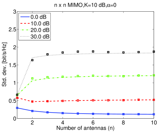
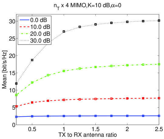
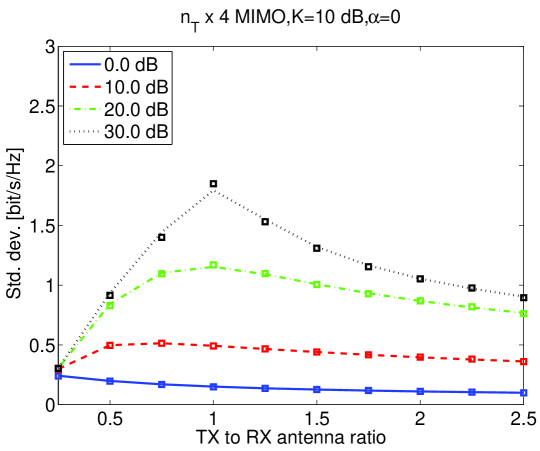
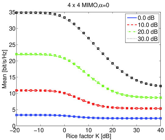
Then, we consider the impact of changing each parameter in turn, with the aim of illustrating the accuracy of the asymptotic approximation proposed. For each parameter we plot the mean and standard deviation of the mutual information by using the asymptotic method (solid lines) and Monte-Carlo simulation (markers).

VI-A Impact of the number of antennas

Figures 1 and 2 describe the impact of the number of antennas and of the SNR on the asymptotic approximation accuracy. It can be noticed that the approximation of the mean (ergodic mutual information) is always excellent (the maximum relative error being less than 2%, corresponding to the case of n𝖳=n𝖱=2subscript𝑛𝖳subscript𝑛𝖱2{n_{\mathsf{T}}}={n_{\mathsf{R}}}=2 and SNR =30absent30=30 dB). The accuracy of the standard deviation is very good when the SNR is 00 or 101010 dB (relative error always less than 1%) but only fairly accurate when the SNR is 202020 or 303030 dB (maximum relative error around 5%). However, it must be noted that the impact on the outage mutual information approximation (12) is attenuated by the fact that the standard deviation is considerably smaller than the mean when the SNR is sufficiently large.

VI-B Impact of the antenna ratio

Figures 3 and 4 describe the impact of the TX to RX antenna ratio and of the SNR on the asymptotic approximation accuracy. It is assumed that the number of receive antenna is fixed, n𝖱=4subscript𝑛𝖱4{n_{\mathsf{R}}}=4, and the number of transmit antennas ranges from n𝖳=1subscript𝑛𝖳1{n_{\mathsf{T}}}=1 to 101010. Both the mean and the standard deviation of the mutual information display very good accuracy with a maximum relative error smaller than 2%.

VI-C Impact of the Rice factor

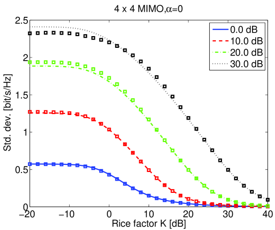
Figures 5 and 6 describe the impact of the Rice factor and of the SNR on the asymptotic approximation accuracy. It can be noticed that the ergodic capacity accuracy is always very good in the cases observed (maximum relative error around 1%) while the standard deviation is slightly overestimated for low K𝐾K (maximum relative error around 4%) and underestimated higher K𝐾K (the threshold depending on the SNR). This effect can be explained by considering that the low K𝐾K condition entails a larger amount of randomness in the channel matrix that increases the asymptotic variance expression. The deviation is larger for high SNR, as in the previous cases observed. Again, the error on the standard deviation has a modest relative impact on the outage mutual information which is the goal of the variance approximation.

VI-D Impact of spatial correlation

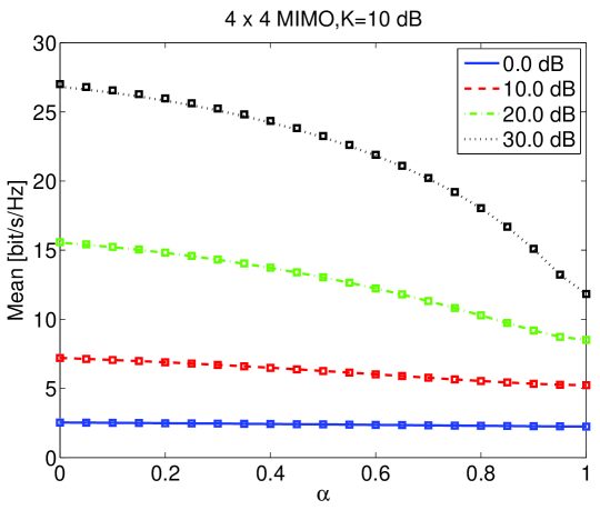
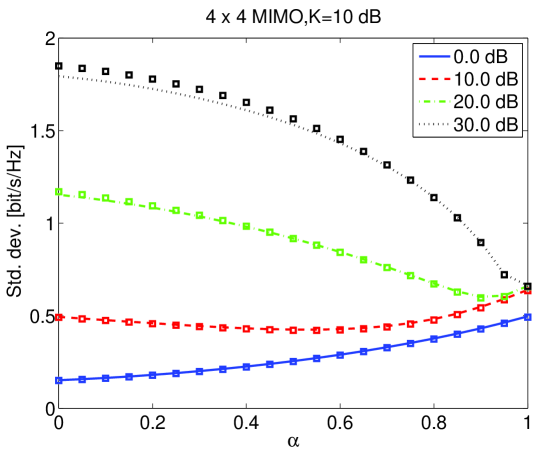
Figures 7 and 8 describe the impact of spatial correlation of the SNR on the asymptotic approximation accuracy. The relative error remains below 1%percent11\% for the ergodic capacity and 3%percent33\% for the standard deviation. The relative error increases as the SNR increases and correlation decreases.

It is interesting to note that spatial correlation has a minor effect at moderate SNR, whereas it becomes important as the SNR increases.


Summarizing the numerical results obtained so far we can say that randomness tends to increase the relative error between the analytic asymptotic approximation and the actual value (obtained via Monte-Carlo simulation). So, increasing the SNR and decreasing the correlation or the Rice factor produces an increase of randomness that entails a larger relative error. Besides this, it can be noticed that the relative error gets larger as the antenna ratio gets closer to 111. Finally, the relative error decreases as the number of antennas increases but this is a trivial consequence of the fact that the approximation is asymptotic in the number of antennas.

VI-E Outage mutual information

In order to assess the accuracy of the proposed asymptotic approximation we consider here the outage mutual information, defined implicitly as follows:

IϵsupR>0{R:P(I(𝐇)<R)<ϵ}.subscript𝐼italic-ϵsubscriptsupremum𝑅0conditional-set𝑅𝑃𝐼𝐇𝑅italic-ϵI_{\epsilon}\triangleq\sup_{R>0}\Big{\{}R~{}:~{}P(I(\mathbf{H})<R)<\epsilon\Big{\}}. (18)

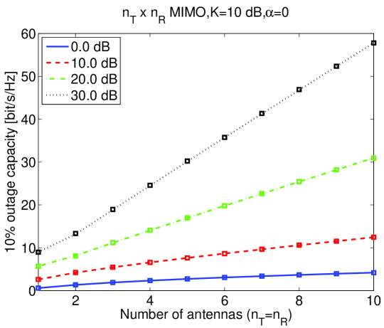
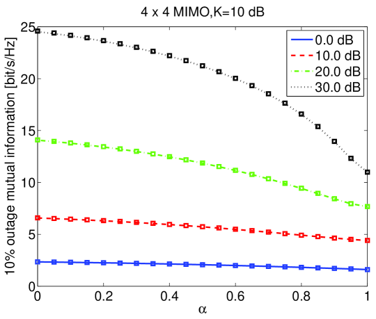
We compare the asymptotic analytic approximation (12) against the exact numerical result obtained by accurate (though lengthy) Monte-Carlo simulation. The results are illustrated in Figs. 9 and 10, reporting I10%subscript𝐼percent10I_{10\%} (i.e., the 10%percent1010\% outage mutual information) versus the number of antennas and the exponential correlation base α𝛼\alpha, respectively. The maximum relative error is around 1%percent11\% in the cases considered, with the maximum corresponding to the case of 2×2222\times 2 MIMO with the largest SNR. This is comparable with the relative error already found for the ergodic capacity approximation.

VII Conclusions

This paper presented an analytic approach, based on the replica method, allowing to approximate the statistics of the mutual information for a separately correlated Rician fading MIMO channel. We showed that the mutual information statistics approach the Gaussian distribution as the number of transmit and receive antennas grows large, with their ratio approaching a finite constant.

More specifically, we saw that the mutual information mean (corresponding to the ergodic mutual information of the channel) yields a very accurate approximation of the real value (which was obtained by extensive Monte-Carlo simulation) with a relative error never larger than a few percent units. This remarkable accuracy was obtained not only with a large number of antennas but also in cases when the number of antennas is definitely small, even in the limiting SISO case! As a result, the asymptotic analysis becomes a valuable tool to assess the system performance whenever this has to be done analytically, such as in the case of covariance optimization with the goal of finding the channel capacity. This application is illustrated in the paper by considering the uncorrelated Rician fading channel.

We also showed that the mutual information standard deviation approximation is very good. This is important in view of the application of these results to the derivation of the outage mutual information. We showed that the outage mutual information, obtained by using the asymptotic mean and standard deviation, is very accurate in the cases considered, since the relative error is always lower than 1%. This result depends on the asymptotic Gaussianity of the mutual information, which is proven in the paper.

Summarizing, the analytic approach presented allows to address concisely the performance of realistic models of MIMO channels (based on separately correlated Rician fading). The accuracy obtained is sufficient for most applications and eliminates the need to run computer intensive simulations or implement numerical methods in orderto optimize the system performance. Many applications of this asymptotic method are appearing in the conference literature. Among them, it is worth mentioning the optimization of the transmitted signal covariance, with and without interference, and the derivation of the capacity region of the multiuser multiple access MIMO channel. A simple example of the former (relevant to the case of uncorrelated Rician fading without interference) is given in the paper.

VIII Acknowledgments

The author would like to thank the Associate Editor and the Reviewers for the constructive comments and suggestions, which allowed him to improve the quality of the original submission. Additionally, the author wishes to acknowledge several useful discussions with Dr. Erwin Riegler.

-A Property of the Kronecker product

Property -A.1

For any matrices 𝐀,𝐗,𝐁,𝐘𝐀𝐗𝐁𝐘\mathbf{A},\mathbf{X},\mathbf{B},\mathbf{Y} such that the product 𝐀𝐗H𝐁𝐘𝐀𝐗𝐻𝐁𝐘\mathbf{A}\mathbf{X}{H}\mathbf{B}\mathbf{Y} exists and is a square matrix, we have:

𝗧𝗿(𝐀𝐗H𝐁𝐘)=vec(𝐗)H(𝐀T𝐁)vec(𝐘).𝗧𝗿𝐀𝐗𝐻𝐁𝐘vec𝐗𝐻tensor-product𝐀𝑇𝐁vec𝐘\mathop{\mathsfbf{Tr}}(\mathbf{A}\mathbf{X}{H}\mathbf{B}\mathbf{Y})=\mathrm{vec}(\mathbf{X}){H}(\mathbf{A}{T}\otimes\mathbf{B})\mathrm{vec}(\mathbf{Y}).
Proof.

Assume that 𝐗=(𝐱1,,𝐱m)𝐗subscript𝐱1subscript𝐱𝑚\mathbf{X}=(\mathbf{x}_{1},\ldots,\mathbf{x}_{m}) and 𝐘=(𝐲1,,𝐲n)𝐘subscript𝐲1subscript𝐲𝑛\mathbf{Y}=(\mathbf{y}_{1},\ldots,\mathbf{y}_{n}). Then,

𝗧𝗿(𝐀𝐗H𝐁𝐘)𝗧𝗿𝐀𝐗𝐻𝐁𝐘\displaystyle\mathop{\mathsfbf{Tr}}(\mathbf{A}\mathbf{X}{H}\mathbf{B}\mathbf{Y}) =\displaystyle= 𝗧𝗿[𝐀(𝐱1H𝐁𝐲1𝐱1H𝐁𝐲n𝐱mH𝐁𝐲1𝐱mH𝐁𝐲n)]𝗧𝗿delimited-[]𝐀superscriptsubscript𝐱1𝐻subscript𝐁𝐲1superscriptsubscript𝐱1𝐻subscript𝐁𝐲𝑛superscriptsubscript𝐱𝑚𝐻subscript𝐁𝐲1superscriptsubscript𝐱𝑚𝐻subscript𝐁𝐲𝑛\displaystyle\mathop{\mathsfbf{Tr}}\left[\mathbf{A}\left(\begin{array}[]{ccc}\mathbf{x}_{1}^{H}\mathbf{B}\mathbf{y}_{1}&\cdots&\mathbf{x}_{1}^{H}\mathbf{B}\mathbf{y}_{n}\\ \vdots&\ddots&\vdots\\ \mathbf{x}_{m}^{H}\mathbf{B}\mathbf{y}_{1}&\cdots&\mathbf{x}_{m}^{H}\mathbf{B}\mathbf{y}_{n}\\ \end{array}\right)\right]
=\displaystyle= a,b(𝐀)a,b𝐱bH𝐁𝐲a=ba𝐱bH(𝐀)a,b𝐁𝐲asubscript𝑎𝑏subscript𝐀𝑎𝑏superscriptsubscript𝐱𝑏𝐻subscript𝐁𝐲𝑎subscript𝑏subscript𝑎superscriptsubscript𝐱𝑏𝐻subscript𝐀𝑎𝑏subscript𝐁𝐲𝑎\displaystyle\sum_{a,b}(\mathbf{A})_{a,b}\mathbf{x}_{b}^{H}\mathbf{B}\mathbf{y}_{a}=\sum_{b}\sum_{a}\mathbf{x}_{b}^{H}(\mathbf{A})_{a,b}\mathbf{B}\mathbf{y}_{a}
=\displaystyle= vec(𝐗)H(𝐀T𝐁)vec(𝐘).vecsuperscript𝐗𝐻tensor-product𝐀𝑇𝐁vec𝐘\displaystyle\mathrm{vec}(\mathbf{X})^{H}(\mathbf{A}{T}\otimes\mathbf{B})\mathrm{vec}(\mathbf{Y}).

-B Integrals

Integral -B.1

For every pair of Hermitian positive definite matrices 𝐀m×m,𝐂n×nformulae-sequence𝐀superscript𝑚𝑚𝐂superscript𝑛𝑛\mathbf{A}\in\mathbb{C}^{m\times m},\mathbf{C}\in\mathbb{C}^{n\times n}, and for any matrices 𝐁,𝐃m×n𝐁𝐃superscript𝑚𝑛\mathbf{B},\mathbf{D}\in\mathbb{C}^{m\times n}, we have:

n×metr[π(𝐀𝐔H𝐂𝐔+𝐁H𝐔+𝐔H𝐃)]𝑑𝐔subscriptsuperscript𝑛𝑚etrdelimited-[]𝜋𝐀𝐔𝐻𝐂𝐔𝐁𝐻𝐔𝐔𝐻𝐃differential-d𝐔\displaystyle\int_{\mathbb{C}^{n\times m}}\mathrm{etr}[-\pi(\mathbf{A}\mathbf{U}{H}\mathbf{C}\mathbf{U}+\mathbf{B}{H}\mathbf{U}+\mathbf{U}{H}\mathbf{D})]d\mathbf{U} =\displaystyle= det(𝐀T𝐂)1etr(π𝐀1𝐁𝐂1𝐃H)superscripttensor-product𝐀𝑇𝐂1etr𝜋superscript𝐀1superscript𝐁𝐂1𝐃𝐻\displaystyle\det(\mathbf{A}{T}\otimes\mathbf{C})^{-1}\mathrm{etr}(\pi\mathbf{A}^{-1}\mathbf{B}\mathbf{C}^{-1}\mathbf{D}{H})
=\displaystyle= det(𝐀)ndet(𝐂)metr(π𝐀1𝐁𝐂1𝐃H).superscript𝐀𝑛superscript𝐂𝑚etr𝜋superscript𝐀1superscript𝐁𝐂1𝐃𝐻\displaystyle\det(\mathbf{A})^{-n}\det(\mathbf{C})^{-m}\mathrm{etr}(\pi\mathbf{A}^{-1}\mathbf{B}\mathbf{C}^{-1}\mathbf{D}{H}).
Proof.

From Property -A.1, we have:

𝗧𝗿(𝐀𝐔H𝐂𝐔)=vec(𝐔)H(𝐀T𝐂)vec(𝐔).𝗧𝗿𝐀𝐔𝐻𝐂𝐔vecsuperscript𝐔𝐻tensor-product𝐀𝑇𝐂vec𝐔\mathop{\mathsfbf{Tr}}(\mathbf{A}\mathbf{U}{H}\mathbf{C}\mathbf{U})=\mathrm{vec}(\mathbf{U})^{H}(\mathbf{A}{T}\otimes\mathbf{C})\mathrm{vec}(\mathbf{U}).

Then, we can write the integral on the lhs of (-B.1) as

mnexp[π(𝐮H𝐏𝐮+𝐛H𝐮+𝐮H𝐝)]𝑑𝐮subscriptsuperscript𝑚𝑛𝜋𝐮𝐻𝐏𝐮𝐛𝐻𝐮𝐮𝐻𝐝differential-d𝐮\int_{\mathbb{C}^{mn}}\exp[-\pi(\mathbf{u}{H}\mathbf{P}\mathbf{u}+\mathbf{b}{H}\mathbf{u}+\mathbf{u}{H}\mathbf{d})]d\mathbf{u}

where 𝐏=𝐀T𝐂𝐏tensor-product𝐀𝑇𝐂\mathbf{P}=\mathbf{A}{T}\otimes\mathbf{C}, 𝐛=vec(𝐁)𝐛vec𝐁\mathbf{b}=\mathrm{vec}(\mathbf{B}), and 𝐝=vec(𝐃)𝐝vec𝐃\mathbf{d}=\mathrm{vec}(\mathbf{D}). Since 𝐀𝐀\mathbf{A} and 𝐂𝐂\mathbf{C} are Hermitian and positive definite by assumption, so are 𝐀T𝐀𝑇\mathbf{A}{T} and 𝐏=𝐀T𝐂𝐏tensor-product𝐀𝑇𝐂\mathbf{P}=\mathbf{A}{T}\otimes\mathbf{C}.

Applying the change of variables 𝐯=𝐏1/2𝐮𝐯superscript𝐏12𝐮\mathbf{v}=\mathbf{P}^{1/2}\mathbf{u}, we obtain:

(det𝐏)1mnexp[π(𝐯H𝐯+𝐛H𝐏1/2𝐯+𝐯H𝐏1/2𝐝)]𝑑𝐯.superscript𝐏1subscriptsuperscript𝑚𝑛𝜋𝐯𝐻𝐯𝐛𝐻superscript𝐏12𝐯𝐯𝐻superscript𝐏12𝐝differential-d𝐯(\det\mathbf{P})^{-1}\int_{\mathbb{C}^{mn}}\exp[-\pi(\mathbf{v}{H}\mathbf{v}+\mathbf{b}{H}\mathbf{P}^{-1/2}\mathbf{v}+\mathbf{v}{H}\mathbf{P}^{-1/2}\mathbf{d})]d\mathbf{v}.

This integral can also be written as

(det𝐏)1a=1mnexp[π(|va|2+b~ava+vad~a)]𝑑vasuperscript𝐏1superscriptsubscriptproduct𝑎1𝑚𝑛subscript𝜋superscriptsubscript𝑣𝑎2superscriptsubscript~𝑏𝑎subscript𝑣𝑎superscriptsubscript𝑣𝑎subscript~𝑑𝑎differential-dsubscript𝑣𝑎(\det\mathbf{P})^{-1}\prod_{a=1}^{mn}\int_{\mathbb{C}}\exp[-\pi(|v_{a}|^{2}+\tilde{b}_{a}^{*}v_{a}+v_{a}^{*}\tilde{d}_{a})]dv_{a}

where we let 𝐛~=𝐏1/2𝐛~𝐛superscript𝐏12𝐛\widetilde{\mathbf{b}}=\mathbf{P}^{-1/2}\mathbf{b} and 𝐝~=𝐏1/2𝐝~𝐝superscript𝐏12𝐝\widetilde{\mathbf{d}}=\mathbf{P}^{-1/2}\mathbf{d}. Setting va=vax+jvaysubscript𝑣𝑎subscript𝑣𝑎𝑥𝑗subscript𝑣𝑎𝑦v_{a}=v_{ax}+jv_{ay}, we have

|va|2+b~ava+vad~a=vax2+vax(b~a+d~a)+vay2+jvay(b~ad~a).superscriptsubscript𝑣𝑎2superscriptsubscript~𝑏𝑎subscript𝑣𝑎superscriptsubscript𝑣𝑎subscript~𝑑𝑎superscriptsubscript𝑣𝑎𝑥2subscript𝑣𝑎𝑥superscriptsubscript~𝑏𝑎subscript~𝑑𝑎superscriptsubscript𝑣𝑎𝑦2𝑗subscript𝑣𝑎𝑦superscriptsubscript~𝑏𝑎subscript~𝑑𝑎|v_{a}|^{2}+\tilde{b}_{a}^{*}v_{a}+v_{a}^{*}\tilde{d}_{a}=v_{ax}^{2}+v_{ax}(\tilde{b}_{a}^{*}+\tilde{d}_{a})+v_{ay}^{2}+jv_{ay}(\tilde{b}_{a}^{*}-\tilde{d}_{a}).

By using repeatedly the standard Gaussian integral

exp[π(x2+ax)]𝑑x=exp(πa2/4),a,formulae-sequencesubscript𝜋superscript𝑥2𝑎𝑥differential-d𝑥𝜋superscript𝑎24𝑎\int_{\mathbb{R}}\exp[-\pi(x^{2}+ax)]dx=\exp(\pi a^{2}/4),\qquad a\in\mathbb{C},

we obtain:

mnexp[π(𝐯H𝐯+𝐛H𝐏1/2𝐯+𝐯H𝐏1/2𝐛)]𝑑𝐯subscriptsuperscript𝑚𝑛𝜋𝐯𝐻𝐯𝐛𝐻superscript𝐏12𝐯𝐯𝐻superscript𝐏12𝐛differential-d𝐯\displaystyle\int_{\mathbb{C}^{mn}}\exp[-\pi(\mathbf{v}{H}\mathbf{v}+\mathbf{b}{H}\mathbf{P}^{-1/2}\mathbf{v}+\mathbf{v}{H}\mathbf{P}^{-1/2}\mathbf{b})]d\mathbf{v}
=\displaystyle= a=1mn{exp[π(b~a+d~a)2/4]exp[π(b~ad~a)2/4]}superscriptsubscriptproduct𝑎1𝑚𝑛𝜋superscriptsuperscriptsubscript~𝑏𝑎subscript~𝑑𝑎24𝜋superscriptsuperscriptsubscript~𝑏𝑎subscript~𝑑𝑎24\displaystyle\prod_{a=1}^{mn}\Big{\{}\exp[\pi(\tilde{b}_{a}^{*}+\tilde{d}_{a})^{2}/4]\exp[-\pi(\tilde{b}_{a}^{*}-\tilde{d}_{a})^{2}/4]\Big{\}}
=\displaystyle= a=1mnexp(πb~ad~a)=exp(π𝐛~H𝐝~)=exp(π𝐛H𝐏1𝐝).superscriptsubscriptproduct𝑎1𝑚𝑛𝜋superscriptsubscript~𝑏𝑎subscript~𝑑𝑎𝜋~𝐛𝐻~𝐝𝜋𝐛𝐻superscript𝐏1𝐝\displaystyle\prod_{a=1}^{mn}\exp(\pi\tilde{b}_{a}^{*}\tilde{d}_{a})=\exp(\pi\widetilde{\mathbf{b}}{H}\widetilde{\mathbf{d}})=\exp(\pi\mathbf{b}{H}\mathbf{P}^{-1}\mathbf{d}).

Finally, since 𝐏1=(𝐀1)T𝐂1superscript𝐏1tensor-productsuperscript𝐀1𝑇superscript𝐂1\mathbf{P}^{-1}=(\mathbf{A}^{-1}){T}\otimes\mathbf{C}^{-1}, applying Property -A.1 we get:

vec(𝐁)H((𝐀1)T𝐂1)vec(𝐃)=𝗧𝗿(𝐀1𝐁𝐂1𝐃H),vec𝐁𝐻tensor-productsuperscript𝐀1𝑇superscript𝐂1vec𝐃𝗧𝗿superscript𝐀1superscript𝐁𝐂1𝐃𝐻\mathrm{vec}(\mathbf{B}){H}((\mathbf{A}^{-1}){T}\otimes\mathbf{C}^{-1})\mathrm{vec}(\mathbf{D})=\mathop{\mathsfbf{Tr}}(\mathbf{A}^{-1}\mathbf{B}\mathbf{C}^{-1}\mathbf{D}{H}),

which in turn leads to (-B.1). ∎

Remark .1

Ref. [34, eq.(124)] reports the following incorrect result:

𝑑rexp(rv)jexp(rtut)dt2πj=exp(uv)u,v.formulae-sequencesubscriptdifferential-d𝑟𝑟𝑣subscriptj𝑟𝑡𝑢𝑡𝑑𝑡2𝜋j𝑢𝑣𝑢𝑣\int_{\mathbb{R}}dr\exp(-rv)\int_{\mathrm{j}\,\mathbb{R}}\exp(rt-ut)\frac{dt}{2\pi\mathrm{j}\,}=\exp(-uv)\qquad u,v\in\mathbb{C}. (24)

The previous result is wrong because the function exp(rv)𝑟𝑣\exp(-rv) is not a test function for the δ𝛿\delta-sequence δA(ru)=AAexp(j(ru)t)dt2πsubscript𝛿𝐴𝑟𝑢superscriptsubscript𝐴𝐴j𝑟𝑢𝑡𝑑𝑡2𝜋\delta_{A}(r-u)=\int_{-A}^{A}\exp(\mathrm{j}\,(r-u)t)\frac{dt}{2\pi} (unless v𝑣v is purely imaginary) since it is unbounded over the integration domain of r𝑟r [26]. However, if we smoothen the test function by it by a suitable Gaussian factor, we obtain:

+jr0𝑑rt0+jexp{αr2+βt2+rtutrv}dt2πj=11+4αβexp(uvαu2+βv21+4αβ).subscriptjsubscript𝑟0differential-d𝑟subscriptsubscript𝑡0j𝛼superscript𝑟2𝛽superscript𝑡2𝑟𝑡𝑢𝑡𝑟𝑣𝑑𝑡2𝜋j114𝛼𝛽𝑢𝑣𝛼superscript𝑢2𝛽superscript𝑣214𝛼𝛽\int_{\mathbb{R}+\mathrm{j}\,r_{0}}dr\int_{t_{0}+\mathrm{j}\,\mathbb{R}}\exp\Big{\{}-\alpha r^{2}+\beta t^{2}+rt-ut-rv\Big{\}}\frac{dt}{2\pi\mathrm{j}\,}=\frac{1}{\sqrt{1+4\alpha\beta}}\exp\bigg{(}\frac{-uv-\alpha u^{2}+\beta v^{2}}{1+4\alpha\beta}\bigg{)}. (25)

This is a Lebesgue integral provided that α,β>0𝛼𝛽0\alpha,\beta>0 and it holds for any r0,t0subscript𝑟0subscript𝑡0r_{0},t_{0}\in\mathbb{R}. Therefore, we can replace eq. (24) by:

exp(uv)=limα,β0+jr0𝑑rt0+jexp{αr2+βt2+rtutrv}dt2πj.𝑢𝑣subscript𝛼𝛽0subscriptjsubscript𝑟0differential-d𝑟subscriptsubscript𝑡0j𝛼superscript𝑟2𝛽superscript𝑡2𝑟𝑡𝑢𝑡𝑟𝑣𝑑𝑡2𝜋j\exp(-uv)=\lim_{\alpha,\beta\downarrow 0}\int_{\mathbb{R}+\mathrm{j}\,r_{0}}dr\int_{t_{0}+\mathrm{j}\,\mathbb{R}}\exp\Big{\{}-\alpha r^{2}+\beta t^{2}+rt-ut-rv\Big{\}}\frac{dt}{2\pi\mathrm{j}\,}. (26)

The previous result allows us to prove the following proposition.

Integral -B.2

(Robust Hubbard–Stratonovich transformation) For every pair of matrices 𝐀m×n,𝐁n×mformulae-sequence𝐀superscript𝑚𝑛𝐁superscript𝑛𝑚\mathbf{A}\in\mathbb{C}^{m\times n},\mathbf{B}\in\mathbb{C}^{n\times m}, we have:

etr(𝐀𝐁)=limα,β0etr(α𝐖𝐖T+β𝐙𝐙T+𝐖𝐙𝐀𝐖𝐁𝐙)𝑑μ(𝐖,𝐙)etr𝐀𝐁subscript𝛼𝛽0etr𝛼𝐖𝐖𝑇𝛽𝐙𝐙𝑇𝐖𝐙𝐀𝐖𝐁𝐙differential-d𝜇𝐖𝐙\mathrm{etr}(-\mathbf{A}\mathbf{B})=\lim_{\alpha,\beta\downarrow 0}\int\mathrm{etr}(-\alpha\mathbf{W}\mathbf{W}{T}+\beta\mathbf{Z}\mathbf{Z}{T}+\mathbf{W}\mathbf{Z}-\mathbf{A}\mathbf{W}-\mathbf{B}\mathbf{Z})d\mu(\mathbf{W},\mathbf{Z}) (27)

where dμ(𝐖,𝐙)=a=1nb=1m12πjd(𝐖)abd(𝐙)ba𝑑𝜇𝐖𝐙superscriptsubscriptproduct𝑎1𝑛superscriptsubscriptproduct𝑏1𝑚12𝜋𝑗𝑑subscript𝐖𝑎𝑏𝑑subscript𝐙𝑏𝑎d\mu(\mathbf{W},\mathbf{Z})=\prod_{a=1}^{n}\prod_{b=1}^{m}\frac{1}{2\pi j}d(\mathbf{W})_{ab}d(\mathbf{Z})_{ba} and integration is carried out along contours parallel to the real axis for each (𝐖)absubscript𝐖𝑎𝑏(\mathbf{W})_{ab} and to the imaginary axis for each (𝐙)basubscript𝐙𝑏𝑎(\mathbf{Z})_{ba}.

Proof.

The proof stems from repeated application of (26). ∎

-C Proof of Theorem IV.1

Proof.

Using the complete expansion in (8), we can write the CGF as:666 Here we used the series expansion (1+x)1exp(xx2/2)=1+k=3ckxk=113x3+14x415x5+29x61984x7+superscript1𝑥1𝑥superscript𝑥221superscriptsubscript𝑘3subscript𝑐𝑘superscript𝑥𝑘113superscript𝑥314superscript𝑥415superscript𝑥529superscript𝑥61984superscript𝑥7(1+x)^{-1}\exp(x-x^{2}/2)=1+\sum_{k=3}^{\infty}c_{k}x^{k}=1-\frac{1}{3}x^{3}+\frac{1}{4}x^{4}-\frac{1}{5}x^{5}+\frac{2}{9}x^{6}-\frac{19}{84}x^{7}+\dots.

g(ν)𝑔𝜈\displaystyle g(\nu) similar-to\displaystyle\sim ν[wˇzˇlndet(𝐈n𝖱+wˇ𝐑𝐇~𝐇~H𝐈n𝖳+zˇ𝐓~)]𝜈delimited-[]ˇ𝑤ˇ𝑧matrixsubscript𝐈subscript𝑛𝖱ˇ𝑤𝐑~𝐇~𝐇𝐻subscript𝐈subscript𝑛𝖳ˇ𝑧~𝐓\displaystyle\nu\left[\check{w}\check{z}-\ln\det\begin{pmatrix}\mathbf{I}_{{n_{\mathsf{R}}}}+\check{w}\mathbf{R}&\widetilde{\mathbf{H}}\\ -\widetilde{\mathbf{H}}{H}&\mathbf{I}_{{n_{\mathsf{T}}}}+\check{z}\widetilde{\mathbf{T}}\end{pmatrix}\right]
+ln{1(2π)ν2etr[12{αˇ𝐔2βˇ𝐕2+2jγˇ𝐔𝐕}]\displaystyle+\ln\bigg{\{}\int\frac{1}{(2\pi)^{\nu^{2}}}~{}\mathrm{etr}\bigg{[}\frac{1}{2}\Big{\{}\check{\alpha}\mathbf{U}^{2}-\check{\beta}\mathbf{V}^{2}+2\,j\,\check{\gamma}\mathbf{U}\mathbf{V}\Big{\}}\bigg{]}
{1+k=3ck𝗧𝗿[(𝐔(𝐀1𝐑)j𝐕(𝐁1𝐓~)𝐔(𝐂1𝐑)j𝐕(𝐃1𝐓~))k]}d𝐔d𝐕}.\displaystyle\cdot\left\{1+\sum_{k=3}^{\infty}c_{k}\mathop{\mathsfbf{Tr}}\left[\begin{pmatrix}\mathbf{U}\otimes(\mathbf{A}_{1}\mathbf{R})&j\mathbf{V}\otimes(\mathbf{B}_{1}\widetilde{\mathbf{T}})\\ \mathbf{U}\otimes(\mathbf{C}_{1}\mathbf{R})&j\mathbf{V}\otimes(\mathbf{D}_{1}\widetilde{\mathbf{T}})\end{pmatrix}^{k}\right]\right\}d\mathbf{U}d\mathbf{V}\bigg{\}}.

Thus, in order to prove the convergence of g(ν)𝑔𝜈g(\nu) to the Gaussian CGF, we have to show that, as n𝖱subscript𝑛𝖱{n_{\mathsf{R}}}\to\infty,

etr[12{αˇ𝐔2βˇ𝐕2+2jγˇ𝐔𝐕}]𝗧𝗿[(𝐔(𝐀1𝐑)j𝐕(𝐁1𝐓~)𝐔(𝐂1𝐑)j𝐕(𝐃1𝐓~))k]d𝐔d𝐕0etrdelimited-[]12ˇ𝛼superscript𝐔2ˇ𝛽superscript𝐕22𝑗ˇ𝛾𝐔𝐕𝗧𝗿delimited-[]superscriptmatrixtensor-product𝐔subscript𝐀1𝐑tensor-product𝑗𝐕subscript𝐁1~𝐓tensor-product𝐔subscript𝐂1𝐑tensor-product𝑗𝐕subscript𝐃1~𝐓𝑘𝑑𝐔𝑑𝐕0\int\mathrm{etr}\bigg{[}\frac{1}{2}\Big{\{}\check{\alpha}\mathbf{U}^{2}-\check{\beta}\mathbf{V}^{2}+2\,j\,\check{\gamma}\mathbf{U}\mathbf{V}\Big{\}}\bigg{]}\mathop{\mathsfbf{Tr}}\left[\begin{pmatrix}\mathbf{U}\otimes(\mathbf{A}_{1}\mathbf{R})&j\mathbf{V}\otimes(\mathbf{B}_{1}\widetilde{\mathbf{T}})\\ \mathbf{U}\otimes(\mathbf{C}_{1}\mathbf{R})&j\mathbf{V}\otimes(\mathbf{D}_{1}\widetilde{\mathbf{T}})\end{pmatrix}^{k}\right]d\mathbf{U}d\mathbf{V}\to 0 (28)

for k3𝑘3k\geq 3. Now, in order to balance the asymptotic order of the matrix multipliers of 𝐔𝐔\mathbf{U} and 𝐕𝐕\mathbf{V}, it is convenient to apply the change of variables 𝐔=n𝖱1/2𝐔ˇ𝐔superscriptsubscript𝑛𝖱12ˇ𝐔\mathbf{U}={n_{\mathsf{R}}}^{-1/2}\check{\mathbf{U}} and 𝐕=n𝖱1/2𝐕ˇ𝐕superscriptsubscript𝑛𝖱12ˇ𝐕\mathbf{V}={n_{\mathsf{R}}}^{1/2}\check{\mathbf{V}}. Then, the limit (28) becomes:

etr[12{n𝖱1αˇ𝐔ˇ2n𝖱βˇ𝐕ˇ2+2jγˇ𝐔ˇ𝐕ˇ}]etrdelimited-[]12superscriptsubscript𝑛𝖱1ˇ𝛼superscriptˇ𝐔2subscript𝑛𝖱ˇ𝛽superscriptˇ𝐕22𝑗ˇ𝛾ˇ𝐔ˇ𝐕\displaystyle\int\mathrm{etr}\bigg{[}\frac{1}{2}\Big{\{}{n_{\mathsf{R}}}^{-1}\check{\alpha}\check{\mathbf{U}}^{2}-{n_{\mathsf{R}}}\check{\beta}\check{\mathbf{V}}^{2}+2\,j\,\check{\gamma}\check{\mathbf{U}}\check{\mathbf{V}}\Big{\}}\bigg{]} (29)
𝗧𝗿[(𝐔ˇ(n𝖱1/2𝐀1𝐑)j𝐕ˇ(n𝖱1/2𝐁1𝐓~)𝐔ˇ(n𝖱1/2𝐂1𝐑)j𝐕ˇ(n𝖱1/2𝐃1𝐓~))k]d𝐔ˇd𝐕ˇn𝖱0\displaystyle\cdot\mathop{\mathsfbf{Tr}}\left[\begin{pmatrix}\check{\mathbf{U}}\otimes({n_{\mathsf{R}}}^{-1/2}\mathbf{A}_{1}\mathbf{R})&j\check{\mathbf{V}}\otimes({n_{\mathsf{R}}}^{1/2}\mathbf{B}_{1}\widetilde{\mathbf{T}})\\ \check{\mathbf{U}}\otimes({n_{\mathsf{R}}}^{-1/2}\mathbf{C}_{1}\mathbf{R})&j\check{\mathbf{V}}\otimes({n_{\mathsf{R}}}^{1/2}\mathbf{D}_{1}\widetilde{\mathbf{T}})\end{pmatrix}^{k}\right]d\check{\mathbf{U}}d\check{\mathbf{V}}\stackrel{{\scriptstyle{n_{\mathsf{R}}}\to\infty}}{{\longrightarrow}}0

and since

αˇˇ𝛼\displaystyle\check{\alpha} =\displaystyle= 𝗧𝗿[(𝐀ˇ1𝐑)2]𝗧𝗿(𝐑2)=O(n𝖱),𝗧𝗿delimited-[]superscriptsubscriptˇ𝐀1𝐑2𝗧𝗿superscript𝐑2𝑂subscript𝑛𝖱\displaystyle\mathop{\mathsfbf{Tr}}[(\check{\mathbf{A}}_{1}\mathbf{R})^{2}]\leq\mathop{\mathsfbf{Tr}}(\mathbf{R}^{2})=O({n_{\mathsf{R}}}),
βˇˇ𝛽\displaystyle\check{\beta} =\displaystyle= 𝗧𝗿[(𝐃ˇ1𝐓~)2]𝗧𝗿(𝐓~2)=O(n𝖱1),𝗧𝗿delimited-[]superscriptsubscriptˇ𝐃1~𝐓2𝗧𝗿superscript~𝐓2𝑂superscriptsubscript𝑛𝖱1\displaystyle\mathop{\mathsfbf{Tr}}[(\check{\mathbf{D}}_{1}\widetilde{\mathbf{T}})^{2}]\leq\mathop{\mathsfbf{Tr}}(\widetilde{\mathbf{T}}^{2})=O({n_{\mathsf{R}}}^{-1}),

by the theorem’s assumptions, it is plain to see that condition (29) is equivalent to the limit

𝗧𝗿[(𝐔ˇ(n𝖱1/2𝐀1𝐑)j𝐕ˇ(n𝖱1/2𝐁1𝐓~)𝐔ˇ(n𝖱1/2𝐂1𝐑)j𝐕ˇ(n𝖱1/2𝐃1𝐓~))k]n𝖱0superscriptsubscript𝑛𝖱𝗧𝗿delimited-[]superscriptmatrixtensor-productˇ𝐔superscriptsubscript𝑛𝖱12subscript𝐀1𝐑tensor-product𝑗ˇ𝐕superscriptsubscript𝑛𝖱12subscript𝐁1~𝐓tensor-productˇ𝐔superscriptsubscript𝑛𝖱12subscript𝐂1𝐑tensor-product𝑗ˇ𝐕superscriptsubscript𝑛𝖱12subscript𝐃1~𝐓𝑘0\mathop{\mathsfbf{Tr}}\left[\begin{pmatrix}\check{\mathbf{U}}\otimes({n_{\mathsf{R}}}^{-1/2}\mathbf{A}_{1}\mathbf{R})&j\check{\mathbf{V}}\otimes({n_{\mathsf{R}}}^{1/2}\mathbf{B}_{1}\widetilde{\mathbf{T}})\\ \check{\mathbf{U}}\otimes({n_{\mathsf{R}}}^{-1/2}\mathbf{C}_{1}\mathbf{R})&j\check{\mathbf{V}}\otimes({n_{\mathsf{R}}}^{1/2}\mathbf{D}_{1}\widetilde{\mathbf{T}})\end{pmatrix}^{k}\right]\stackrel{{\scriptstyle{n_{\mathsf{R}}}\to\infty}}{{\longrightarrow}}0 (30)

To prove (30), we investigate the asymptotic order of the singular values of the matrices 𝐀1𝐑subscript𝐀1𝐑\mathbf{A}_{1}\mathbf{R}, 𝐁1𝐓~subscript𝐁1~𝐓\mathbf{B}_{1}\widetilde{\mathbf{T}}, 𝐂1𝐑subscript𝐂1𝐑\mathbf{C}_{1}\mathbf{R}, and 𝐃1𝐓~subscript𝐃1~𝐓\mathbf{D}_{1}\widetilde{\mathbf{T}}. We shall use the following linear algebra inequalities [20]:

σmax(𝐌𝐍)σmax(𝐌)σmax(𝐍),for any 𝐌,𝐍 with compatible sizesσmax(𝐌)σmax(𝐍),for any square 𝐌,𝐍 with 𝐌𝐍𝗧𝗿(𝐌)𝗧𝗿(𝐍),for any square 𝐌,𝐍 with 𝐌𝐍subscript𝜎𝐌𝐍subscript𝜎𝐌subscript𝜎𝐍for any 𝐌,𝐍 with compatible sizessubscript𝜎𝐌subscript𝜎𝐍for any square 𝐌,𝐍 with 𝐌𝐍𝗧𝗿𝐌𝗧𝗿𝐍for any square 𝐌,𝐍 with 𝐌𝐍\begin{array}[]{rcll}\sigma_{\max}(\mathbf{M}\mathbf{N})&\leq&\sigma_{\max}(\mathbf{M})\sigma_{\max}(\mathbf{N}),&\text{for any $\mathbf{M},\mathbf{N}$ with compatible sizes}\\ \sigma_{\max}(\mathbf{M})&\leq&\sigma_{\max}(\mathbf{N}),&\text{for any square $\mathbf{M},\mathbf{N}$ with $\mathbf{M}\leq\mathbf{N}$}\\ \mathop{\mathsfbf{Tr}}(\mathbf{M})&\leq&\mathop{\mathsfbf{Tr}}(\mathbf{N}),&\text{for any square $\mathbf{M},\mathbf{N}$ with $\mathbf{M}\leq\mathbf{N}$}\end{array}

From the asymptotic setting definitions of Section II-B we have the following results.

  1. 1.

    Since

    𝐀1𝐑=[wˇ𝐈n𝖱+𝐑1+𝐑1𝐇~(𝐈n𝖳+zˇ𝐓~)1𝐇~H]1,subscript𝐀1𝐑superscriptdelimited-[]ˇ𝑤subscript𝐈subscript𝑛𝖱superscript𝐑1superscript𝐑1~𝐇superscriptsubscript𝐈subscript𝑛𝖳ˇ𝑧~𝐓1~𝐇𝐻1\mathbf{A}_{1}\mathbf{R}=[\check{w}\mathbf{I}_{{n_{\mathsf{R}}}}+\mathbf{R}^{-1}+\mathbf{R}^{-1}\widetilde{\mathbf{H}}(\mathbf{I}_{{n_{\mathsf{T}}}}+\check{z}\widetilde{\mathbf{T}})^{-1}\widetilde{\mathbf{H}}{H}]^{-1},

    we have 𝐀1𝐑𝐑subscript𝐀1𝐑𝐑\mathbf{A}_{1}\mathbf{R}\leq\mathbf{R}, so that

    σmax(𝐀1𝐑)σmax(𝐑)=Θ(1)andzˇ=𝗧𝗿(𝐀1𝐑)𝗧𝗿(𝐑)=Θ(n𝖱).formulae-sequencesubscript𝜎subscript𝐀1𝐑subscript𝜎𝐑Θ1andˇ𝑧𝗧𝗿subscript𝐀1𝐑𝗧𝗿𝐑Θsubscript𝑛𝖱\sigma_{\max}(\mathbf{A}_{1}\mathbf{R})\leq\sigma_{\max}(\mathbf{R})=\Theta(1)\qquad\text{and}\qquad\check{z}=\mathop{\mathsfbf{Tr}}(\mathbf{A}_{1}\mathbf{R})\leq\mathop{\mathsfbf{Tr}}(\mathbf{R})=\Theta({n_{\mathsf{R}}}).
  2. 2.

    Since

    𝐃1𝐓~=[zˇ𝐈n𝖳+𝐓~1+𝐓~1𝐇~H(𝐈n𝖱+wˇ𝐑)1𝐇~]1,subscript𝐃1~𝐓superscriptdelimited-[]ˇ𝑧subscript𝐈subscript𝑛𝖳superscript~𝐓1superscript~𝐓1~𝐇𝐻superscriptsubscript𝐈subscript𝑛𝖱ˇ𝑤𝐑1~𝐇1\mathbf{D}_{1}\widetilde{\mathbf{T}}=[\check{z}\mathbf{I}_{{n_{\mathsf{T}}}}+\widetilde{\mathbf{T}}^{-1}+\widetilde{\mathbf{T}}^{-1}\widetilde{\mathbf{H}}{H}(\mathbf{I}_{{n_{\mathsf{R}}}}+\check{w}\mathbf{R})^{-1}\widetilde{\mathbf{H}}]^{-1},

    we have 𝐃1𝐓~𝐓~subscript𝐃1~𝐓~𝐓\mathbf{D}_{1}\widetilde{\mathbf{T}}\leq\widetilde{\mathbf{T}}, so that

    σmax(𝐃1𝐓~)σmax(𝐓~)=Θ(n𝖱1)andwˇ=𝗧𝗿(𝐃1𝐓~)𝗧𝗿(𝐓~)=Θ(1).formulae-sequencesubscript𝜎subscript𝐃1~𝐓subscript𝜎~𝐓Θsuperscriptsubscript𝑛𝖱1andˇ𝑤𝗧𝗿subscript𝐃1~𝐓𝗧𝗿~𝐓Θ1\sigma_{\max}(\mathbf{D}_{1}\widetilde{\mathbf{T}})\leq\sigma_{\max}(\widetilde{\mathbf{T}})=\Theta({n_{\mathsf{R}}}^{-1})\qquad\text{and}\qquad\check{w}=\mathop{\mathsfbf{Tr}}(\mathbf{D}_{1}\widetilde{\mathbf{T}})\leq\mathop{\mathsfbf{Tr}}(\widetilde{\mathbf{T}})=\Theta(1).
  3. 3.

    By using the previous inequalities on the maximum singular values we obtain:

    𝗧𝗿[(𝐀1𝐑)k]=O(n𝖱)and𝗧𝗿[(𝐃1𝐓~)k]=O(n𝖱1k)formulae-sequence𝗧𝗿delimited-[]superscriptsubscript𝐀1𝐑𝑘𝑂subscript𝑛𝖱and𝗧𝗿delimited-[]superscriptsubscript𝐃1~𝐓𝑘𝑂superscriptsubscript𝑛𝖱1𝑘\mathop{\mathsfbf{Tr}}[(\mathbf{A}_{1}\mathbf{R})^{k}]=O({n_{\mathsf{R}}})\qquad\text{and}\qquad\mathop{\mathsfbf{Tr}}[(\mathbf{D}_{1}\widetilde{\mathbf{T}})^{k}]=O({n_{\mathsf{R}}}^{1-k})

    which confirms, for k=2𝑘2k=2, that αˇ=O(n𝖱)ˇ𝛼𝑂subscript𝑛𝖱\check{\alpha}=O({n_{\mathsf{R}}}) and βˇ=O(n𝖱1)ˇ𝛽𝑂superscriptsubscript𝑛𝖱1\check{\beta}=O({n_{\mathsf{R}}}^{-1}).

  4. 4.

    Setting 𝐇^(𝐈n𝖱+wˇ𝐑)1/2𝐇~^𝐇superscriptsubscript𝐈subscript𝑛𝖱ˇ𝑤𝐑12~𝐇\widehat{\mathbf{H}}\triangleq(\mathbf{I}_{n_{\mathsf{R}}}+\check{w}\mathbf{R})^{-1/2}\widetilde{\mathbf{H}}, by the definition of 𝐁1subscript𝐁1\mathbf{B}_{1} in (9), we have:

    σmax(𝐁1𝐓~)subscript𝜎subscript𝐁1~𝐓\displaystyle\sigma_{\max}(\mathbf{B}_{1}\widetilde{\mathbf{T}}) =\displaystyle= σmax[(𝐈n𝖱+wˇ𝐑)1/2𝐇^(𝐈n𝖳+zˇ𝐓~+𝐇^H𝐇^)1𝐓~]subscript𝜎delimited-[]superscriptsubscript𝐈subscript𝑛𝖱ˇ𝑤𝐑12^𝐇superscriptsubscript𝐈subscript𝑛𝖳ˇ𝑧~𝐓^𝐇𝐻^𝐇1~𝐓\displaystyle\sigma_{\max}[(\mathbf{I}_{n_{\mathsf{R}}}+\check{w}\mathbf{R})^{-1/2}\widehat{\mathbf{H}}(\mathbf{I}_{n_{\mathsf{T}}}+\check{z}\widetilde{\mathbf{T}}+\widehat{\mathbf{H}}{H}\widehat{\mathbf{H}})^{-1}\widetilde{\mathbf{T}}]
    \displaystyle\leq σmax[(𝐈n𝖱+wˇ𝐑)1/2]σmax[𝐇^(𝐈n𝖳+zˇ𝐓~+𝐇^H𝐇^)1]σmax(𝐓~).subscript𝜎delimited-[]superscriptsubscript𝐈subscript𝑛𝖱ˇ𝑤𝐑12subscript𝜎delimited-[]^𝐇superscriptsubscript𝐈subscript𝑛𝖳ˇ𝑧~𝐓^𝐇𝐻^𝐇1subscript𝜎~𝐓\displaystyle\sigma_{\max}[(\mathbf{I}_{n_{\mathsf{R}}}+\check{w}\mathbf{R})^{-1/2}]\sigma_{\max}[\widehat{\mathbf{H}}(\mathbf{I}_{n_{\mathsf{T}}}+\check{z}\widetilde{\mathbf{T}}+\widehat{\mathbf{H}}{H}\widehat{\mathbf{H}})^{-1}]\sigma_{\max}(\widetilde{\mathbf{T}}).

    Since (plainly) σmax[(𝐈n𝖱+wˇ𝐑)1/2]=O(1)subscript𝜎delimited-[]superscriptsubscript𝐈subscript𝑛𝖱ˇ𝑤𝐑12𝑂1\sigma_{\max}[(\mathbf{I}_{n_{\mathsf{R}}}+\check{w}\mathbf{R})^{-1/2}]=O(1) and

    σmax2[𝐇^(𝐈n𝖳+zˇ𝐓~+𝐇^H𝐇^)1]superscriptsubscript𝜎2delimited-[]^𝐇superscriptsubscript𝐈subscript𝑛𝖳ˇ𝑧~𝐓^𝐇𝐻^𝐇1\displaystyle\sigma_{\max}^{2}[\widehat{\mathbf{H}}(\mathbf{I}_{n_{\mathsf{T}}}+\check{z}\widetilde{\mathbf{T}}+\widehat{\mathbf{H}}{H}\widehat{\mathbf{H}})^{-1}] =\displaystyle= λmax[𝐇^H𝐇^(𝐈n𝖳+zˇ𝐓~+𝐇^H𝐇^)2]subscript𝜆delimited-[]^𝐇𝐻^𝐇superscriptsubscript𝐈subscript𝑛𝖳ˇ𝑧~𝐓^𝐇𝐻^𝐇2\displaystyle\lambda_{\max}[\widehat{\mathbf{H}}{H}\widehat{\mathbf{H}}(\mathbf{I}_{n_{\mathsf{T}}}+\check{z}\widetilde{\mathbf{T}}+\widehat{\mathbf{H}}{H}\widehat{\mathbf{H}})^{-2}]
    \displaystyle\leq λmax[𝐇^H𝐇^(𝐈n𝖳+𝐇^H𝐇^)2]subscript𝜆delimited-[]^𝐇𝐻^𝐇superscriptsubscript𝐈subscript𝑛𝖳^𝐇𝐻^𝐇2\displaystyle\lambda_{\max}[\widehat{\mathbf{H}}{H}\widehat{\mathbf{H}}(\mathbf{I}_{n_{\mathsf{T}}}+\widehat{\mathbf{H}}{H}\widehat{\mathbf{H}})^{-2}]
    =\displaystyle= maxiλi(𝐇^H𝐇^)[1+λi(𝐇^H𝐇^)]214,subscript𝑖subscript𝜆𝑖^𝐇𝐻^𝐇superscriptdelimited-[]1subscript𝜆𝑖^𝐇𝐻^𝐇214\displaystyle\max_{i}\frac{\lambda_{i}(\widehat{\mathbf{H}}{H}\widehat{\mathbf{H}})}{[1+\lambda_{i}(\widehat{\mathbf{H}}{H}\widehat{\mathbf{H}})]^{2}}\leq\frac{1}{4},

    we have

    σmax(𝐁1𝐓~)=O(n𝖱1).subscript𝜎subscript𝐁1~𝐓𝑂superscriptsubscript𝑛𝖱1\sigma_{\max}(\mathbf{B}_{1}\widetilde{\mathbf{T}})=O({n_{\mathsf{R}}}^{-1}).
  5. 5.

    Setting 𝐇^𝐇~(𝐈n𝖳+zˇ𝐓~)1/2^𝐇~𝐇superscriptsubscript𝐈subscript𝑛𝖳ˇ𝑧~𝐓12\widehat{\mathbf{H}}\triangleq\widetilde{\mathbf{H}}(\mathbf{I}_{n_{\mathsf{T}}}+\check{z}\widetilde{\mathbf{T}})^{-1/2}, by the definition of 𝐂1subscript𝐂1\mathbf{C}_{1} in (9), we have:

    σmax(𝐂1𝐑)subscript𝜎subscript𝐂1𝐑\displaystyle\sigma_{\max}(\mathbf{C}_{1}\mathbf{R}) =\displaystyle= σmax[(𝐈n𝖳+zˇ𝐓~)1/2𝐇^H(𝐈n𝖱+wˇ𝐑+𝐇^𝐇^H)1𝐑]subscript𝜎delimited-[]superscriptsubscript𝐈subscript𝑛𝖳ˇ𝑧~𝐓12^𝐇𝐻superscriptsubscript𝐈subscript𝑛𝖱ˇ𝑤𝐑^𝐇^𝐇𝐻1𝐑\displaystyle\sigma_{\max}[(\mathbf{I}_{n_{\mathsf{T}}}+\check{z}\widetilde{\mathbf{T}})^{-1/2}\widehat{\mathbf{H}}{H}(\mathbf{I}_{n_{\mathsf{R}}}+\check{w}\mathbf{R}+\widehat{\mathbf{H}}\widehat{\mathbf{H}}{H})^{-1}\mathbf{R}]
    \displaystyle\leq σmax[(𝐈n𝖳+zˇ𝐓~)1/2]σmax[𝐇^H(𝐈n𝖱+wˇ𝐑+𝐇^𝐇^H)1]σmax(𝐑).subscript𝜎delimited-[]superscriptsubscript𝐈subscript𝑛𝖳ˇ𝑧~𝐓12subscript𝜎delimited-[]^𝐇𝐻superscriptsubscript𝐈subscript𝑛𝖱ˇ𝑤𝐑^𝐇^𝐇𝐻1subscript𝜎𝐑\displaystyle\sigma_{\max}[(\mathbf{I}_{n_{\mathsf{T}}}+\check{z}\widetilde{\mathbf{T}})^{-1/2}]\sigma_{\max}[\widehat{\mathbf{H}}{H}(\mathbf{I}_{n_{\mathsf{R}}}+\check{w}\mathbf{R}+\widehat{\mathbf{H}}\widehat{\mathbf{H}}{H})^{-1}]\sigma_{\max}(\mathbf{R}).

    Since (plainly) σmax[(𝐈n𝖱+zˇ𝐓~)1/2]=O(1)subscript𝜎delimited-[]superscriptsubscript𝐈subscript𝑛𝖱ˇ𝑧~𝐓12𝑂1\sigma_{\max}[(\mathbf{I}_{n_{\mathsf{R}}}+\check{z}\widetilde{\mathbf{T}})^{-1/2}]=O(1) and

    σmax2[𝐇^H(𝐈n𝖱+wˇ𝐑+𝐇^𝐇^H)1]superscriptsubscript𝜎2delimited-[]^𝐇𝐻superscriptsubscript𝐈subscript𝑛𝖱ˇ𝑤𝐑^𝐇^𝐇𝐻1\displaystyle\sigma_{\max}^{2}[\widehat{\mathbf{H}}{H}(\mathbf{I}_{n_{\mathsf{R}}}+\check{w}\mathbf{R}+\widehat{\mathbf{H}}\widehat{\mathbf{H}}{H})^{-1}] =\displaystyle= λmax[𝐇^𝐇^H(𝐈n𝖱+wˇ𝐑+𝐇^𝐇^H)2]subscript𝜆delimited-[]^𝐇^𝐇𝐻superscriptsubscript𝐈subscript𝑛𝖱ˇ𝑤𝐑^𝐇^𝐇𝐻2\displaystyle\lambda_{\max}[\widehat{\mathbf{H}}\widehat{\mathbf{H}}{H}(\mathbf{I}_{n_{\mathsf{R}}}+\check{w}\mathbf{R}+\widehat{\mathbf{H}}\widehat{\mathbf{H}}{H})^{-2}]
    \displaystyle\leq λmax[𝐇^𝐇^H(𝐈n𝖱+𝐇^𝐇^H)2]subscript𝜆delimited-[]^𝐇^𝐇𝐻superscriptsubscript𝐈subscript𝑛𝖱^𝐇^𝐇𝐻2\displaystyle\lambda_{\max}[\widehat{\mathbf{H}}\widehat{\mathbf{H}}{H}(\mathbf{I}_{n_{\mathsf{R}}}+\widehat{\mathbf{H}}\widehat{\mathbf{H}}{H})^{-2}]
    =\displaystyle= maxiλi(𝐇^𝐇^H)[1+λi(𝐇^𝐇^H)]214,subscript𝑖subscript𝜆𝑖^𝐇^𝐇𝐻superscriptdelimited-[]1subscript𝜆𝑖^𝐇^𝐇𝐻214\displaystyle\max_{i}\frac{\lambda_{i}(\widehat{\mathbf{H}}\widehat{\mathbf{H}}{H})}{[1+\lambda_{i}(\widehat{\mathbf{H}}\widehat{\mathbf{H}}{H})]^{2}}\leq\frac{1}{4},

    we have

    σmax(𝐂1𝐑)=O(1).subscript𝜎subscript𝐂1𝐑𝑂1\sigma_{\max}(\mathbf{C}_{1}\mathbf{R})=O(1).

In order to prove (30), notice that the maximum singular values of the matrices on the rhs of the Kronecker products in

(𝐔(n𝖱1/2𝐀1𝐑)j𝐕(n𝖱1/2𝐁1𝐓~)𝐔(n𝖱1/2𝐂1𝐑)j𝐕(n𝖱1/2𝐃1𝐓~))matrixtensor-product𝐔superscriptsubscript𝑛𝖱12subscript𝐀1𝐑tensor-product𝑗𝐕superscriptsubscript𝑛𝖱12subscript𝐁1~𝐓tensor-product𝐔superscriptsubscript𝑛𝖱12subscript𝐂1𝐑tensor-product𝑗𝐕superscriptsubscript𝑛𝖱12subscript𝐃1~𝐓\begin{pmatrix}\mathbf{U}\otimes({n_{\mathsf{R}}}^{-1/2}\mathbf{A}_{1}\mathbf{R})&j\mathbf{V}\otimes({n_{\mathsf{R}}}^{1/2}\mathbf{B}_{1}\widetilde{\mathbf{T}})\\ \mathbf{U}\otimes({n_{\mathsf{R}}}^{-1/2}\mathbf{C}_{1}\mathbf{R})&j\mathbf{V}\otimes({n_{\mathsf{R}}}^{1/2}\mathbf{D}_{1}\widetilde{\mathbf{T}})\end{pmatrix}

are all O(n𝖱1/2)𝑂superscriptsubscript𝑛𝖱12O({n_{\mathsf{R}}}^{-1/2}) as n𝖱subscript𝑛𝖱{n_{\mathsf{R}}}\to\infty. Thus, if we define

(ϕ11,k(𝐔,𝐕)𝐌11,kϕ12,k(𝐔,𝐕)𝐌12,kϕ21,k(𝐔,𝐕)𝐌21,kϕ22,k(𝐔,𝐕)𝐌22,k)(𝐔(n𝖱1/2𝐀1𝐑)j𝐕(n𝖱1/2𝐁1𝐓~)𝐔(n𝖱1/2𝐂1𝐑)j𝐕(n𝖱1/2𝐃1𝐓~))kmatrixtensor-productsubscriptitalic-ϕ11𝑘𝐔𝐕subscript𝐌11𝑘tensor-productsubscriptitalic-ϕ12𝑘𝐔𝐕subscript𝐌12𝑘tensor-productsubscriptitalic-ϕ21𝑘𝐔𝐕subscript𝐌21𝑘tensor-productsubscriptitalic-ϕ22𝑘𝐔𝐕subscript𝐌22𝑘superscriptmatrixtensor-product𝐔superscriptsubscript𝑛𝖱12subscript𝐀1𝐑tensor-product𝑗𝐕superscriptsubscript𝑛𝖱12subscript𝐁1~𝐓tensor-product𝐔superscriptsubscript𝑛𝖱12subscript𝐂1𝐑tensor-product𝑗𝐕superscriptsubscript𝑛𝖱12subscript𝐃1~𝐓𝑘\begin{pmatrix}\phi_{11,k}(\mathbf{U},\mathbf{V})\otimes\mathbf{M}_{11,k}&\phi_{12,k}(\mathbf{U},\mathbf{V})\otimes\mathbf{M}_{12,k}\\ \phi_{21,k}(\mathbf{U},\mathbf{V})\otimes\mathbf{M}_{21,k}&\phi_{22,k}(\mathbf{U},\mathbf{V})\otimes\mathbf{M}_{22,k}\end{pmatrix}\triangleq\begin{pmatrix}\mathbf{U}\otimes({n_{\mathsf{R}}}^{-1/2}\mathbf{A}_{1}\mathbf{R})&j\mathbf{V}\otimes({n_{\mathsf{R}}}^{1/2}\mathbf{B}_{1}\widetilde{\mathbf{T}})\\ \mathbf{U}\otimes({n_{\mathsf{R}}}^{-1/2}\mathbf{C}_{1}\mathbf{R})&j\mathbf{V}\otimes({n_{\mathsf{R}}}^{1/2}\mathbf{D}_{1}\widetilde{\mathbf{T}})\end{pmatrix}^{k}

we have σmax(𝐌ij,k)=O(n𝖱k/2)subscript𝜎subscript𝐌𝑖𝑗𝑘𝑂superscriptsubscript𝑛𝖱𝑘2\sigma_{\max}(\mathbf{M}_{ij,k})=O({n_{\mathsf{R}}}^{-k/2}). Therefore, the trace

𝗧𝗿(ϕ11,k(𝐔,𝐕))𝗧𝗿(𝐌11,k)+𝗧𝗿(ϕ22,k(𝐔,𝐕))𝗧𝗿(𝐌22,k)=O(n𝖱1k/2)𝗧𝗿subscriptitalic-ϕ11𝑘𝐔𝐕𝗧𝗿subscript𝐌11𝑘𝗧𝗿subscriptitalic-ϕ22𝑘𝐔𝐕𝗧𝗿subscript𝐌22𝑘𝑂superscriptsubscript𝑛𝖱1𝑘2\mathop{\mathsfbf{Tr}}(\phi_{11,k}(\mathbf{U},\mathbf{V}))\mathop{\mathsfbf{Tr}}(\mathbf{M}_{11,k})+\mathop{\mathsfbf{Tr}}(\phi_{22,k}(\mathbf{U},\mathbf{V}))\mathop{\mathsfbf{Tr}}(\mathbf{M}_{22,k})=O({n_{\mathsf{R}}}^{1-k/2})

approaches 00 as n𝖱subscript𝑛𝖱{n_{\mathsf{R}}}\to\infty for all k3𝑘3k\geq 3, which proves (28) and the fact that g(ν)𝑔𝜈g(\nu) converges to a Gaussian CGF.

-D Uniqueness of the solution of eqs. (10)

The proof reported here was inspired by a similar proof included in [17].

Proof.

Eqs. (10) can be written equivalently as follows:

{1=ψ^1(w,z)𝗧𝗿(𝐃1𝐓~)w=𝗧𝗿{[wz𝐈n𝖳+w𝐓~1+w𝐓~1𝐇~H(𝐈n𝖱+w𝐑)1𝐇~]1}1=ψ^2(w,z)𝗧𝗿(𝐀1𝐓~)z=𝗧𝗿{[wz𝐈n𝖱+z𝐑1+z𝐑1𝐇~(𝐈n𝖳+z𝐓~)1𝐇~H]1}cases1subscript^𝜓1𝑤𝑧𝗧𝗿subscript𝐃1~𝐓𝑤𝗧𝗿superscriptdelimited-[]𝑤𝑧subscript𝐈subscript𝑛𝖳𝑤superscript~𝐓1𝑤superscript~𝐓1~𝐇𝐻superscriptsubscript𝐈subscript𝑛𝖱𝑤𝐑1~𝐇11subscript^𝜓2𝑤𝑧𝗧𝗿subscript𝐀1~𝐓𝑧𝗧𝗿superscriptdelimited-[]𝑤𝑧subscript𝐈subscript𝑛𝖱𝑧superscript𝐑1𝑧superscript𝐑1~𝐇superscriptsubscript𝐈subscript𝑛𝖳𝑧~𝐓1~𝐇𝐻1\left\{\begin{array}[]{lllll}1&=&\hat{\psi}_{1}(w,z)&\triangleq&\displaystyle\frac{\mathop{\mathsfbf{Tr}}(\mathbf{D}_{1}\widetilde{\mathbf{T}})}{w}=\mathop{\mathsfbf{Tr}}\Big{\{}[wz\mathbf{I}_{{n_{\mathsf{T}}}}+w\widetilde{\mathbf{T}}^{-1}+w\widetilde{\mathbf{T}}^{-1}\widetilde{\mathbf{H}}{H}(\mathbf{I}_{{n_{\mathsf{R}}}}+w\mathbf{R})^{-1}\widetilde{\mathbf{H}}]^{-1}\Big{\}}\\[8.53581pt] 1&=&\hat{\psi}_{2}(w,z)&\triangleq&\displaystyle\frac{\mathop{\mathsfbf{Tr}}(\mathbf{A}_{1}\widetilde{\mathbf{T}})}{z}=\mathop{\mathsfbf{Tr}}\Big{\{}[wz\mathbf{I}_{{n_{\mathsf{R}}}}+z\mathbf{R}^{-1}+z\mathbf{R}^{-1}\widetilde{\mathbf{H}}(\mathbf{I}_{{n_{\mathsf{T}}}}+z\widetilde{\mathbf{T}})^{-1}\widetilde{\mathbf{H}}{H}]^{-1}\Big{\}}\end{array}\right. (31)

First, we calculate the partial derivatives of these functions with respect to w𝑤w and z𝑧z:

{ψ^1w=𝗧𝗿{𝐃1𝐓~𝐃1[𝐈n𝖳+z𝐓~+𝐇~H(𝐈n𝖱+w𝐑)2𝐇~]}w2<0ψ^1z=𝗧𝗿{(𝐃1𝐓~)2}w<0ψ^2w=𝗧𝗿{(𝐀1𝐑)2}z<0ψ^2z=𝗧𝗿{𝐀1𝐑𝐀1[𝐈n𝖱+w𝐑+𝐇~(𝐈n𝖳+z𝐓~)2𝐇~H]}z2<0casessubscript^𝜓1𝑤𝗧𝗿subscript𝐃1~𝐓subscript𝐃1delimited-[]subscript𝐈subscript𝑛𝖳𝑧~𝐓~𝐇𝐻superscriptsubscript𝐈subscript𝑛𝖱𝑤𝐑2~𝐇superscript𝑤20subscript^𝜓1𝑧𝗧𝗿superscriptsubscript𝐃1~𝐓2𝑤0subscript^𝜓2𝑤𝗧𝗿superscriptsubscript𝐀1𝐑2𝑧0subscript^𝜓2𝑧𝗧𝗿subscript𝐀1subscript𝐑𝐀1delimited-[]subscript𝐈subscript𝑛𝖱𝑤𝐑~𝐇superscriptsubscript𝐈subscript𝑛𝖳𝑧~𝐓2~𝐇𝐻superscript𝑧20\left\{\begin{array}[]{lll}\displaystyle\frac{\partial\hat{\psi}_{1}}{\partial w}&=&\displaystyle-\frac{\mathop{\mathsfbf{Tr}}\{\mathbf{D}_{1}\widetilde{\mathbf{T}}\mathbf{D}_{1}[\mathbf{I}_{{n_{\mathsf{T}}}}+z\widetilde{\mathbf{T}}+\widetilde{\mathbf{H}}{H}(\mathbf{I}_{{n_{\mathsf{R}}}}+w\mathbf{R})^{-2}\widetilde{\mathbf{H}}]\}}{w^{2}}<0\\ \displaystyle\frac{\partial\hat{\psi}_{1}}{\partial z}&=&\displaystyle-\frac{\mathop{\mathsfbf{Tr}}\{(\mathbf{D}_{1}\widetilde{\mathbf{T}})^{2}\}}{w}<0\\ \displaystyle\frac{\partial\hat{\psi}_{2}}{\partial w}&=&\displaystyle-\frac{\mathop{\mathsfbf{Tr}}\{(\mathbf{A}_{1}\mathbf{R})^{2}\}}{z}<0\\ \displaystyle\frac{\partial\hat{\psi}_{2}}{\partial z}&=&\displaystyle-\frac{\mathop{\mathsfbf{Tr}}\{\mathbf{A}_{1}\mathbf{R}\mathbf{A}_{1}[\mathbf{I}_{{n_{\mathsf{R}}}}+w\mathbf{R}+\widetilde{\mathbf{H}}(\mathbf{I}_{{n_{\mathsf{T}}}}+z\widetilde{\mathbf{T}})^{-2}\widetilde{\mathbf{H}}{H}]\}}{z^{2}}<0\end{array}\right. (32)

Then, we notice that ψ^1(0,z)=subscript^𝜓10𝑧\hat{\psi}_{1}(0,z)=\infty, ψ^1(,z)=0subscript^𝜓1𝑧0\hat{\psi}_{1}(\infty,z)=0, and ψ^1/w<0subscript^𝜓1𝑤0\partial\hat{\psi}_{1}/\partial w<0. Hence, ψ^1(w,z)subscript^𝜓1𝑤𝑧\hat{\psi}_{1}(w,z) is a continuous monotonically decreasing function in w𝑤w and the equation ψ^1(w,z)=1subscript^𝜓1𝑤𝑧1\hat{\psi}_{1}(w,z)=1 has a single solution w=g(z)[0,)𝑤𝑔𝑧0w=g(z)\in[0,\infty), which is a continuous function of z𝑧z by the Implicit Function Theorem [27, Th. 3.16]. Moreover, from the first of (31) and from the first two inequalities of (32), we obtain:

g(z)=ψ^1/zψ^1/w<0.superscript𝑔𝑧subscript^𝜓1𝑧subscript^𝜓1𝑤0g^{\prime}(z)=-\frac{\partial\hat{\psi}_{1}/\partial z}{\partial\hat{\psi}_{1}/\partial w}<0.

Then, the uniqueness of the solution of (10) requires that the equation h(z)ψ^2(g(z),z)=1𝑧subscript^𝜓2𝑔𝑧𝑧1h(z)\triangleq\hat{\psi}_{2}(g(z),z)=1 has a single solution. This result stems from the fact that ψ^2(g(0),0)=+subscript^𝜓2𝑔00\hat{\psi}_{2}(g(0),0)=+\infty, ψ^2(g(),)=0subscript^𝜓2𝑔0\hat{\psi}_{2}(g(\infty),\infty)=0, and

h(z)=[ψ^2wg(z)+ψ^2z]w=g(z)<0.superscript𝑧subscriptdelimited-[]subscript^𝜓2𝑤superscript𝑔𝑧subscript^𝜓2𝑧𝑤𝑔𝑧0h^{\prime}(z)=\bigg{[}\frac{\partial\hat{\psi}_{2}}{\partial w}g^{\prime}(z)+\frac{\partial\hat{\psi}_{2}}{\partial z}\bigg{]}_{w=g(z)}<0.

The last inequality is equivalent to

[ψ^1wψ^2zψ^1zψ^2w]w=g(z)>0subscriptdelimited-[]subscript^𝜓1𝑤subscript^𝜓2𝑧subscript^𝜓1𝑧subscript^𝜓2𝑤𝑤𝑔𝑧0\bigg{[}\frac{\partial\hat{\psi}_{1}}{\partial w}\frac{\partial\hat{\psi}_{2}}{\partial z}-\frac{\partial\hat{\psi}_{1}}{\partial z}\frac{\partial\hat{\psi}_{2}}{\partial w}\bigg{]}_{w=g(z)}>0

which can be checked by direct substitution of the relevant expressions. ∎

-E Saddlepoint approximation

Here we report some basic facts about saddlepoint approximation. A full account on the subject can be found in [23]. In its simplest form, saddlepoint approximation deals with integrals of the type

I=g(x)exp[λh(x)]𝑑x𝐼subscript𝑔𝑥𝜆𝑥differential-d𝑥I=\int_{\mathbb{R}}g(x)\exp[-\lambda h(x)]dx

in the limit for λ𝜆\lambda\to\infty. Assuming g(x)𝑔𝑥g(x) bounded and h(x)𝑥h(x) with a global minimum at x=x0𝑥subscript𝑥0x=x_{0}, the integral can be approximated, for λ𝜆\lambda\to\infty, as:

Ig(x0)exp[λh(x0)λh′′(x0)(xx0)2/2]𝑑x=2πλh′′(x0)g(x0)exp[λh(x0)].𝐼subscript𝑔subscript𝑥0𝜆subscript𝑥0𝜆superscript′′subscript𝑥0superscript𝑥subscript𝑥022differential-d𝑥2𝜋𝜆superscript′′subscript𝑥0𝑔subscript𝑥0𝜆subscript𝑥0I\approx\int_{\mathbb{R}}g(x_{0})\exp[-\lambda h(x_{0})-\lambda h^{\prime\prime}(x_{0})(x-x_{0})^{2}/2]dx=\sqrt{\frac{2\pi}{\lambda h^{\prime\prime}(x_{0})}}g(x_{0})\exp[-\lambda h(x_{0})].

A more refined derivation yields

I=exp[λh(x0)]λh′′(x0)/(2π){g(x0)+g(5h′′′3h′′2hiv)12gh′′h′′′+12g′′h′′2]24h′′3|x=x01λ+O(1λ2)}.I=\frac{\exp[-\lambda h(x_{0})]}{\sqrt{\lambda h^{\prime\prime}(x_{0})/(2\pi)}}\bigg{\{}g(x_{0})+\frac{g(5h^{\prime\prime\prime}-3h^{\prime\prime 2}h^{iv})-12g^{\prime}h^{\prime\prime}h^{\prime\prime\prime}+12g^{\prime\prime}h^{\prime\prime 2}]}{24h^{\prime\prime 3}}\bigg{|}_{x=x_{0}}\frac{1}{\lambda}+O\bigg{(}\frac{1}{\lambda^{2}}\bigg{)}\bigg{\}}.

This result can be extended to a multidimensional contour integral

I=g(𝐱)exp[λh(𝐱)]𝑑𝐱.𝐼𝑔𝐱𝜆𝐱differential-d𝐱I=\int g(\mathbf{x})\exp[-\lambda h(\mathbf{x})]d\mathbf{x}.

Assuming |g(𝐱)|𝑔𝐱|g(\mathbf{x})| bounded and h(𝐱)𝐱h(\mathbf{x}) real, smooth, and with a global minimum at 𝐱=𝐱0𝐱subscript𝐱0\mathbf{x}=\mathbf{x}_{0}, we have, for λ𝜆\lambda\to\infty:

Ig(𝐱0)exp[λh(𝐱0)λ(𝐱𝐱0)T𝐇0(𝐱𝐱0)/2]𝑑𝐱=g(𝐱0)exp[λh(𝐱0)]det[λ𝐇0/(2π)],𝐼𝑔subscript𝐱0𝜆subscript𝐱0𝜆𝐱subscript𝐱0𝑇subscript𝐇0𝐱subscript𝐱02differential-d𝐱𝑔subscript𝐱0𝜆subscript𝐱0delimited-[]𝜆subscript𝐇02𝜋I\approx\int g(\mathbf{x}_{0})\exp[-\lambda h(\mathbf{x}_{0})-\lambda(\mathbf{x}-\mathbf{x}_{0}){T}\mathbf{H}_{0}(\mathbf{x}-\mathbf{x}_{0})/2]d\mathbf{x}=\frac{g(\mathbf{x}_{0})\exp[-\lambda h(\mathbf{x}_{0})]}{\sqrt{\det[\lambda\mathbf{H}_{0}/(2\pi)]}},

where 𝐇0subscript𝐇0\mathbf{H}_{0} is the Hessian matrix of h(𝐱)𝐱h(\mathbf{x}) at 𝐱=𝐱0𝐱subscript𝐱0\mathbf{x}=\mathbf{x}_{0}, which is assumed to be positive definite.

-F Proof of the inequalities 0<γˇ2αˇβˇ<10superscriptˇ𝛾2ˇ𝛼ˇ𝛽10<\check{\gamma}^{2}-\check{\alpha}\check{\beta}<1

Proof.

First, we show that 0<γˇ<10ˇ𝛾10<\check{\gamma}<1, so that, since αˇβˇ>0ˇ𝛼ˇ𝛽0\check{\alpha}\check{\beta}>0, we have γˇ2αˇβˇ<1superscriptˇ𝛾2ˇ𝛼ˇ𝛽1\check{\gamma}^{2}-\check{\alpha}\check{\beta}<1.

  • The inequality γˇ<1ˇ𝛾1\check{\gamma}<1 derives from

    γˇ=1+𝗧𝗿(𝐁ˇ1𝐓~𝐂ˇ1𝐑)=1𝗧𝗿(𝐑1/2𝐂ˇ1H𝐓~𝐂ˇ1𝐑1/2)=1𝐓~1/2𝐂ˇ1𝐑1/22.ˇ𝛾1𝗧𝗿subscriptˇ𝐁1~𝐓subscriptˇ𝐂1𝐑1𝗧𝗿superscript𝐑12subscriptˇ𝐂1𝐻~𝐓subscriptˇ𝐂1superscript𝐑121superscriptnormsuperscript~𝐓12subscriptˇ𝐂1superscript𝐑122\check{\gamma}=1+\mathop{\mathsfbf{Tr}}(\check{\mathbf{B}}_{1}\widetilde{\mathbf{T}}\check{\mathbf{C}}_{1}\mathbf{R})=1-\mathop{\mathsfbf{Tr}}(\mathbf{R}^{1/2}\check{\mathbf{C}}_{1}{H}\widetilde{\mathbf{T}}\check{\mathbf{C}}_{1}\mathbf{R}^{1/2})=1-\|\widetilde{\mathbf{T}}^{1/2}\check{\mathbf{C}}_{1}\mathbf{R}^{1/2}\|^{2}.
  • The inequality γˇ>0ˇ𝛾0\check{\gamma}>0 derives from

    γˇˇ𝛾\displaystyle\check{\gamma} =\displaystyle= 1+𝗧𝗿(𝐁ˇ1𝐓~𝐂ˇ1𝐑)1𝗧𝗿subscriptˇ𝐁1~𝐓subscriptˇ𝐂1𝐑\displaystyle 1+\mathop{\mathsfbf{Tr}}(\check{\mathbf{B}}_{1}\widetilde{\mathbf{T}}\check{\mathbf{C}}_{1}\mathbf{R})
    =\displaystyle= 1𝗧𝗿[𝐀ˇ1𝐇~(𝐈n𝖳+zˇ𝐓~)1𝐓~(𝐈n𝖳+zˇ𝐓~)1𝐇~H𝐀ˇ1𝐑]1𝗧𝗿delimited-[]subscriptˇ𝐀1~𝐇superscriptsubscript𝐈subscript𝑛𝖳ˇ𝑧~𝐓1~𝐓superscriptsubscript𝐈subscript𝑛𝖳ˇ𝑧~𝐓1~𝐇𝐻subscriptˇ𝐀1𝐑\displaystyle 1-\mathop{\mathsfbf{Tr}}[\check{\mathbf{A}}_{1}\widetilde{\mathbf{H}}(\mathbf{I}_{n_{\mathsf{T}}}+\check{z}\widetilde{\mathbf{T}})^{-1}\widetilde{\mathbf{T}}(\mathbf{I}_{n_{\mathsf{T}}}+\check{z}\widetilde{\mathbf{T}})^{-1}\widetilde{\mathbf{H}}{H}\check{\mathbf{A}}_{1}\mathbf{R}]
    (i)superscript𝑖\displaystyle\stackrel{{\scriptstyle(i)}}{{\geq}} 1zˇ1𝗧𝗿[𝐀ˇ1𝐇~(𝐈n𝖳+zˇ𝐓~)1𝐇~H𝐀ˇ1𝐑]1superscriptˇ𝑧1𝗧𝗿delimited-[]subscriptˇ𝐀1~𝐇superscriptsubscript𝐈subscript𝑛𝖳ˇ𝑧~𝐓1~𝐇𝐻subscriptˇ𝐀1𝐑\displaystyle 1-\check{z}^{-1}\mathop{\mathsfbf{Tr}}[\check{\mathbf{A}}_{1}\widetilde{\mathbf{H}}(\mathbf{I}_{n_{\mathsf{T}}}+\check{z}\widetilde{\mathbf{T}})^{-1}\widetilde{\mathbf{H}}{H}\check{\mathbf{A}}_{1}\mathbf{R}]
    =(ii)superscript𝑖𝑖\displaystyle\stackrel{{\scriptstyle(ii)}}{{=}} 1zˇ1𝗧𝗿[(𝐈n𝖱𝐀ˇ1(𝐈n𝖱+wˇ𝐑))𝐀ˇ1𝐑]1superscriptˇ𝑧1𝗧𝗿delimited-[]subscript𝐈subscript𝑛𝖱subscriptˇ𝐀1subscript𝐈subscript𝑛𝖱ˇ𝑤𝐑subscriptˇ𝐀1𝐑\displaystyle 1-\check{z}^{-1}\mathop{\mathsfbf{Tr}}[(\mathbf{I}_{n_{\mathsf{R}}}-\check{\mathbf{A}}_{1}(\mathbf{I}_{n_{\mathsf{R}}}+\check{w}\mathbf{R}))\check{\mathbf{A}}_{1}\mathbf{R}]
    =(iii)superscript𝑖𝑖𝑖\displaystyle\stackrel{{\scriptstyle(iii)}}{{=}} 𝗧𝗿(𝐀ˇ12𝐑)+wˇαˇzˇ,𝗧𝗿superscriptsubscriptˇ𝐀12𝐑ˇ𝑤ˇ𝛼ˇ𝑧\displaystyle\frac{\mathop{\mathsfbf{Tr}}(\check{\mathbf{A}}_{1}^{2}\mathbf{R})+\check{w}\check{\alpha}}{\check{z}},

    from (i)𝑖(i) the matrix inequality (𝐈n𝖳+zˇ𝐓~)1𝐓~<zˇ1𝐈n𝖳superscriptsubscript𝐈subscript𝑛𝖳ˇ𝑧~𝐓1~𝐓superscriptˇ𝑧1subscript𝐈subscript𝑛𝖳(\mathbf{I}_{n_{\mathsf{T}}}+\check{z}\widetilde{\mathbf{T}})^{-1}\widetilde{\mathbf{T}}<\check{z}^{-1}\mathbf{I}_{n_{\mathsf{T}}}; (ii)𝑖𝑖(ii) the definition of 𝐀ˇ1subscriptˇ𝐀1\check{\mathbf{A}}_{1}; and (iii)𝑖𝑖𝑖(iii) the definition of αˇ=𝗧𝗿(𝐀ˇ1𝐑)ˇ𝛼𝗧𝗿subscriptˇ𝐀1𝐑\check{\alpha}=\mathop{\mathsfbf{Tr}}(\check{\mathbf{A}}_{1}\mathbf{R}). Now, in order to handle the case of singular 𝐑𝐑\mathbf{R}, we define the positive definite matrix 𝐑ϵϵ𝐈n𝖱+𝐑subscript𝐑italic-ϵitalic-ϵsubscript𝐈subscript𝑛𝖱𝐑\mathbf{R}_{\epsilon}\triangleq\epsilon\mathbf{I}_{n_{\mathsf{R}}}+\mathbf{R} for ϵ>0italic-ϵ0\epsilon>0. We have:

    γˇˇ𝛾\displaystyle\check{\gamma} \displaystyle\geq 𝗧𝗿(𝐀ˇ12𝐑ϵ)ϵ𝗧𝗿(𝐀ˇ12)+wˇαˇzˇ𝗧𝗿superscriptsubscriptˇ𝐀12subscript𝐑italic-ϵitalic-ϵ𝗧𝗿superscriptsubscriptˇ𝐀12ˇ𝑤ˇ𝛼ˇ𝑧\displaystyle\frac{\mathop{\mathsfbf{Tr}}(\check{\mathbf{A}}_{1}^{2}\mathbf{R}_{\epsilon})-\epsilon\mathop{\mathsfbf{Tr}}(\check{\mathbf{A}}_{1}^{2})+\check{w}\check{\alpha}}{\check{z}} (33)
    (i)superscript𝑖\displaystyle\stackrel{{\scriptstyle(i)}}{{\geq}} λmin(𝐑ϵ1)𝗧𝗿(𝐀ˇ1𝐑ϵ𝐀ˇ1𝐑ϵ)ϵ𝗧𝗿(𝐀ˇ12)+wˇαˇzˇsubscript𝜆superscriptsubscript𝐑italic-ϵ1𝗧𝗿subscriptˇ𝐀1subscript𝐑italic-ϵsubscriptˇ𝐀1subscript𝐑italic-ϵitalic-ϵ𝗧𝗿superscriptsubscriptˇ𝐀12ˇ𝑤ˇ𝛼ˇ𝑧\displaystyle\frac{\lambda_{\min}(\mathbf{R}_{\epsilon}^{-1})\mathop{\mathsfbf{Tr}}(\check{\mathbf{A}}_{1}\mathbf{R}_{\epsilon}\check{\mathbf{A}}_{1}\mathbf{R}_{\epsilon})-\epsilon\mathop{\mathsfbf{Tr}}(\check{\mathbf{A}}_{1}^{2})+\check{w}\check{\alpha}}{\check{z}}
    (ii)superscript𝑖𝑖\displaystyle\stackrel{{\scriptstyle(ii)}}{{\to}} λmax(𝐑)1+wˇzˇαˇsubscript𝜆superscript𝐑1ˇ𝑤ˇ𝑧ˇ𝛼\displaystyle\frac{\lambda_{\max}(\mathbf{R})^{-1}+\check{w}}{\check{z}}\check{\alpha}
    >\displaystyle> 0,0\displaystyle 0,

    from (i)𝑖(i) the inequality 𝗧𝗿(𝐔𝐕)λmin(𝐔)𝗧𝗿(𝐕)𝗧𝗿𝐔𝐕subscript𝜆𝐔𝗧𝗿𝐕\mathop{\mathsfbf{Tr}}(\mathbf{U}\mathbf{V})\geq\lambda_{\min}(\mathbf{U})\mathop{\mathsfbf{Tr}}(\mathbf{V}) (holding for nonnegative definite matrices 𝐔,𝐕𝐔𝐕\mathbf{U},\mathbf{V} as a direct consequence of [29, 9.H.1.h]); and (ii)𝑖𝑖(ii) taking the limit for ϵ0italic-ϵ0\epsilon\downarrow 0 of the previous lower bound and the limit limϵ0λmin(𝐑ϵ)=λmax(𝐑)1subscriptitalic-ϵ0subscript𝜆subscript𝐑italic-ϵsubscript𝜆superscript𝐑1\lim_{\epsilon\downarrow 0}\lambda_{\min}(\mathbf{R}_{\epsilon})=\lambda_{\max}(\mathbf{R})^{-1}.

The second part of the proof can be accomplished by combining the inequality

γˇλmax(𝐑)1+wˇzˇαˇ>wˇzˇαˇ,ˇ𝛾subscript𝜆superscript𝐑1ˇ𝑤ˇ𝑧ˇ𝛼ˇ𝑤ˇ𝑧ˇ𝛼\check{\gamma}\geq\frac{\lambda_{\max}(\mathbf{R})^{-1}+\check{w}}{\check{z}}\check{\alpha}>\frac{\check{w}}{\check{z}}\check{\alpha},

deriving from (33), and

γˇλmax(𝐓~)1+zˇwˇβˇ>zˇwˇβˇ,ˇ𝛾subscript𝜆superscript~𝐓1ˇ𝑧ˇ𝑤ˇ𝛽ˇ𝑧ˇ𝑤ˇ𝛽\check{\gamma}\geq\frac{\lambda_{\max}(\widetilde{\mathbf{T}})^{-1}+\check{z}}{\check{w}}\check{\beta}>\frac{\check{z}}{\check{w}}\check{\beta},

which can be obtained in a similar way. Multiplying the two inequalities yields γˇ2αˇβˇ>0superscriptˇ𝛾2ˇ𝛼ˇ𝛽0\check{\gamma}^{2}-\check{\alpha}\check{\beta}>0. ∎

References

  • [1] N. Bleistein and R.A. Handelsman, Asymptotic Expansions of Integrals . Dover, 1986
  • [2] T.M. Cover and J.A. Thomas, Elements of Information Theory (2nd Ed.). New York: Wiley, 2006.
  • [3] X.W. Cui, Q.T. Zhang, and Z.M. Feng, “Generic procedure for tightly bounding the capacity of MIMO correlated Rician fading channels,” IEEE Trans. on Commun., vol. 53, no. 5, pp. 890–898, May 2005.
  • [4] P.F. Driessen and G.J. Foschini, “On the capacity formula for multiple input multiple output wireless channels: A geometric interpretation,” IEEE Trans. on Communications, vol. 47, no. 2, pp. 173–176, Feb. 1999.
  • [5] J. Dumont, P. Loubaton, S. Lasaulce, and M. Debbah, “On the asymptotic performance of MIMO correlated Rician channels,” ICASSP 2005, pp. V-813–816, Philadelphia, PA, USA, March 18–23, 2005.
  • [6] J. Dumont, P. Loubaton, S. Lasaulce, “On the capacity achieving transmit covariance matrices of MIMO correlated Rician channels: A large system approach,” Proc. Globecom 2006, San Francisco, Nov. 27-Dec. 1, 2006.
  • [7] S.F. Edwards and P.W. Anderson, “Theory of spin glasses,” J. Phys. F: Metal Physics, vol. 5, pp. 965–974, 1975.
  • [8] M. Elia and G. Taricco, “Integration of the exponential function of a complex quadratic form,” Applied Mathematics E-Notes, vol. 3, pp. 95-98, 2003.
  • [9] F.R. Farrokhi, G.J. Foschini, A. Lozano, and R.A. Valenzuela, “Link-optimal space time processing with multiple transmit and receive antennas,” IEEE Commun. Lett., vol. 5, no. 3, pp. 85–87, March 2001.
  • [10] K.H. Fischer and J.A. Hertz, Spin Glasses. Cambridge University Press, 1991.
  • [11] G.J. Foschini, “Layered space-time architecture for wireless communication in fading environments when using multi-element antennas,” Bell Labs Tech. J., pp. 41–59, 1996.
  • [12] D. Gesbert, H. Bölcskei, D.A. Gore, and A.J. Paulraj, “Outdoor MIMO wireless channels: Models and performance prediction,” IEEE Trans. Commun., vol. 50, no. 12, pp. 1926–1934, Dec. 2002.
  • [13] A.J. Goldsmith, S.A. Jafar , N. Jindal, and S. Vishwanath, “Capacity Limits of MIMO Channels,” IEEE J. Select. Areas Commun., vol. 21, no. 5, pp. 684–702, June 2003.
  • [14] D. Guo and S. Verdú, “Randomly spread CDMA: Asymptotics via statistical physics,” IEEE Trans. Inform. Theory, vol. 51, no. 6, pp. 1983–2010, June 2005.
  • [15] W. Hachem, P. Loubaton, and J. Najim, “The mutual information of a MIMO channel: A survey,” ISCCSP 2006.
  • [16] W. Hachem, P. Loubaton, and J. Najim, “Deterministic equivalents for certain functionals of large random matrices,” Annals of Applied Probability, vol. 17 no. 3, pp. 875–930, 2007.
  • [17] W. Hachem, O. Khorunzhiy, P. Loubaton, J. Najim, and L. Pastur, “A New Approach for Capacity Analysis of Large Dimensional Multi-Antenna Channels,” submitted to IEEE Transactions on Information Theory, December 2006.
  • [18] J. Hansen and H. Bölcskei, “A geometrical investigation of the rank-1 Rician MIMO channel at high SNR,” ISIT 2004, Chicago, USA, June 27 July 2, 2004.
  • [19] D. Hösli, Y.-H. Kim, and A. Lapidoth, “Monotonicity results for coherent MIMO Rician Channels,” IEEE Trans. Inform. Theory, vol. 51, no. 12, pp. 4334–4339, Dec. 2005.
  • [20] R. Horn and C. Johnson, Matrix Analysis. New York: Cambridge University Press, 1985.
  • [21] S.A. Jafar and A. Goldsmith, “Transmitter optimization and optimality of beamforming for multiple antenna systems,” Trans. Wireless Commun., vol. 3, no. 4, pp. 1165–1175, July 2004.
  • [22] S.K. Jayaweera and H.V. Poor, “On the capacity of multiple-antenna systems in Rician fading,” IEEE Transactions on Wireless Communications, vol. 4, no. 3, pp. 1102–1111, March 2005.
  • [23] J.L. Jensen, Saddlepoint Approximations. New York: Oxford University Press, 1995.
  • [24] E. Jorswieck and H. Boche, “Channel capacity and capacity-range of beamforming in MIMO wireless systems under correlated fading with covariance feedback,” IEEE Trans. Wireless Commun., vol. 3, no. 5, pp. 1543–1553, Sept. 2004.
  • [25] M. Kang and M.-S. Alouini, “Capacity of MIMO Rician channels,” IEEE Transactions on Wireless Communications, vol. 5, no. 1, pp. 112–122, January 2006.
  • [26] R.P. Kanwal, Generalized Functions: Theory and Techniques. New York: Academic Press, 1983.
  • [27] A.W. Knapp, Basic Real Analysis. Boston: Birkhäuser, 2005.
  • [28] G. Lebrun, M. Faulkner, M. Shafi, and P.J. Smith, “MIMO Ricean channel capacity; An asymptotic analysis,” IEEE Transactions on Wireless Communications, vol. 5, no. 6, pp. 1343–1350, June 2006.
  • [29] A.W. Marshall and I. Olkin, Inequalities: Theory of Majorization and Its Application. London, U.K.: Academic, 1979.
  • [30] C. Martin and B. Ottersten, “Asymptotic eigenvalue distributions and capacity for MIMO channels under correlated fading,” IEEE Transactions on Wireless Communications, vol. 3, no. 4, pp. 1350 1359, July 2004.
  • [31] M.R. McKay and I.B. Collings, “General capacity bounds for spatially correlated Rician MIMO channels,” IEEE Trans. Inform. Theory, vol. 51, no. 9, pp. 3121–3145, Sept. 2005.
  • [32] M.R. McKay and I.B. Collings, “Improved general lower bound for spatially-correlated Rician MIMO capacity,” IEEE Commun. Letters, vol. 10, no. 3, pp. 162–164, March 2006.
  • [33] M.R. McKay, P.J. Smith, and I.B. Collings, “New Properties of Complex Noncentral Quadratic Forms and Bounds on MIMO Mutual Information,” Proc. IEEE ISIT 2006, Seattle, USA, July 2006, pp. 1209–1213.
  • [34] A.L. Moustakas, S.H. Simon, A.M. Sengupta, “MIMO capacity through correlated channels in the presence of correlated interferers and noise: A (not so) large N𝑁N analysis,” IEEE Trans. Inform. Theory, vol. 49, no. 10, pp. 2545–2561, Oct. 2003.
  • [35] A.L. Moustakas, S.H. Simon, “Random matrix theory of multi-antenna communications: The Rician channel”, J. Phys. A: Math. Gen., vol. 38, pp. 10859–10872, Nov. 2005.
  • [36] A.L. Moustakas, S.H. Simon, “On the Outage Capacity of Correlated Multiple-Path MIMO Channels,” IEEE Trans. Inform. Theory, vol. 53, no. 11, pp. 3887–3903, Nov. 2007.
  • [37] R.R. Müller, “Channel capacity and minimum probability of error in large dual antenna array systems with binary modulation,” IEEE Trans. Sig. Proc., vol. 51, no. 11, pp. 2821–2828, Nov. 2003.
  • [38] R.R. Müller and W.H. Gerstacker, “On the capacity loss due to separation of detection and decoding,” IEEE Trans. Inf. Theory, vol. 50, no. 8, pp. 1769–1778, Aug. 2004.
  • [39] H. Nishimori, Statistical physics of spin glasses and information processing: An introduction. Oxford Univ. Press, 2001.
  • [40] E. Riegler and G. Taricco, “Second-order statistics of the mutual information of the asymptotic separately-correlated Rician fading MIMO channel with interference,” Proc. Globecom 2007, Washington, DC, USA, November 26–30, 2007.
  • [41] E. Riegler and G. Taricco, “On the ergodic capacity region of the separately correlated Rician fading multiple access MIMO channel,” Proc. Globecom 2007, Washington, DC, USA, November 26–30, 2007.
  • [42] A.M. Sayeed, “Deconstructing multiantenna fading channels,” IEEE Trans. Sig. Proc., vol. 50, no. 10, pp. 2563–2579, Oct. 2002.
  • [43] T. Tanaka, “A statistical-mechanics approach to large-system analysis of CDMA multiuser detectors,” IEEE Trans. Inform. Theory vol. 48, no. 11, pp. 2888–910, Nov. 2002.
  • [44] G. Taricco, “On the capacity of separately-correlated MIMO Rician fading channels,” Proc. Globecom 2006, San Francisco, USA, Nov. 27-Dec. 1, 2006.
  • [45] G. Taricco and E. Riegler, “On the ergodic capacity of the asymptotic separately-correlated Rician fading MIMO channel with interference,” in IEEE ISIT 2007, Nice, France, June 24–30, 2007.
  • [46] I. E. Telatar, “Capacity of multi-antenna Gaussian channels,” AT&T Bell Laboratories Technical Report, BL0112170-950615-07TM, June 1995. Also published as “Capacity of multi-antenna Gaussian channels,” European Trans. Telecomm., vol. 10, no. 6, pp. 585–595, November–December 1999.
  • [47] S. Venkatesan, S.H. Simon, and R.A. Valenzuela, “Capacity of a Gaussian MIMO Channel with nonzero mean,” Proc. of IEEE Vehicular Technology Conference, Oct. 2003.
  • [48] M. Vu and A. Paulraj, “Capacity optimization for Rician correlated MIMO wireless channels,” Asilomar Conference 2005, ASilomar CA, USA, Nov. 2005.
  • [49] C.-K. Wen and K.-K. Wong, “Asymptotic analysis of spatially correlated MIMO multiple-access channels with arbitrary signaling inputs for joint and separate decoding,” submitted to IEEE Trans. on Information Theory, 2006.
  • [50] J. Winters, “On the capacity of radio communication systems with diversity in a Rayleigh fading environment,” IEEE J. Select. Areas Commun., vol. 5, no. 6, pp. 871–878, June 1987.
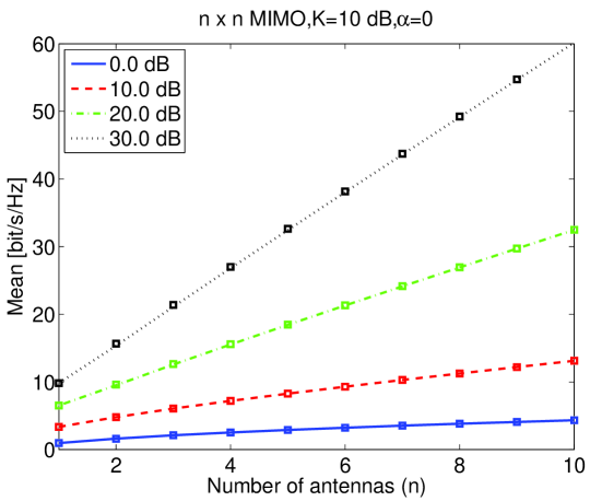
Refer to caption
Figure 1: Capacity mean versus number of antennas for different SNR’s.
Refer to caption
Figure 2: Capacity standard deviation versus number of antennas for different SNR’s.
Refer to caption
Figure 3: Capacity mean versus the TX to RX antenna ratio for different SNR’s.
Refer to caption
Figure 4: Capacity standard deviation versus the TX to RX antenna ratio for different SNR’s.
Refer to caption
Figure 5: Capacity mean versus the Rice factor K𝐾K (expressed in dB) for different SNR’s.
Refer to caption
Figure 6: Capacity standard deviation versus the Rice factor K𝐾K (expressed in dB) for different SNR’s.
Refer to caption
Figure 7: Capacity mean versus exponential spatial correlation base α𝛼\alpha for different SNR’s.
Refer to caption
Figure 8: Capacity standard deviation versus exponential spatial correlation base α𝛼\alpha for different SNR’s.
Refer to caption
Figure 9: Outage capacity versus number of antennas for different SNR’s.
Refer to caption
Figure 10: Outage capacity versus exponential spatial correlation base α𝛼\alpha for different SNR’s.