Two Fractal Overlap Time Series: Earthquakes and Market Crashes

Abstract

We find prominent similarities in the features of the time series for the (model earthquakes or) overlap of two Cantor sets when one set moves with uniform relative velocity over the other and time series of stock prices. An anticipation method for some of the crashes have been proposed here, based on these observations.

I Introduction

Capturing dynamical patterns of stock prices are major challenges both for epistemologists as well as for financial analysts CCB:book . The statistical properties of their (time) variations or fluctuations CCB:book are now well studied and characterized (with established fractal properties), but are not very useful for studying and anticipating their dynamics in the market. Noting that a single fractal gives essentially a time averaged picture, a minimal two-fractal overlap time series model was introduced CCB:Chakrabarti:1999 ; CCB:Pradhan:2003 ; CCB:Pradhan:2004 to capture the time series of earthquake magnitudes. We find that the same model can be used to mimic and study the essential features of the time series of stock prices.

II The two fractal-overlap model of earthquake

Let us consider first a geometric model CCB:Chakrabarti:1999 ; CCB:Pradhan:2003 ; CCB:Pradhan:2004 ; CCB:Bhattacharyya:2005 of the fault dynamics occurring in overlapping tectonic plates that form the earth’s lithosphere. A geological fault is created by a fracture in the earth’s rock layers followed by a displacement of one part relative to the other. The two surfaces of the fault are known to be self-similar fractals. In the model considered here CCB:Chakrabarti:1999 ; CCB:Pradhan:2003 ; CCB:Pradhan:2004 ; CCB:Bhattacharyya:2005 , a fault is represented by a pair of overlapping identical fractals and the fault dynamics arising out of the relative motion of the associated tectonic plates is represented by sliding one of the fractals over the other; the overlap $O$ between the two fractals represents the energy released in an earthquake whereas $\log O$ represents the magnitude of the earthquake. In the simplest form of the model each of the two identical fractals is represented by a regular Cantor set of fractal dimension $\log 2/\log 3$ (see Fig. 1). This is the only exactly solvable model for earthquakes known so far. The exact analysis of this model CCB:Bhattacharyya:2005 for a finite generation $n$ of the Cantor sets with periodic boundary conditions showed that the probability of the overlap $O$, which assumes the values $O=2^{n-k}(k=0,\ldots,n)$, follows the binomial distribution $F$ of $\log_{2}O=n-k$ CCB:Bhattacharyya:2006 :

$$\Pr\left(O=2^{n-k}\right)\equiv\Pr\left(\log_{2}O=n-k\right)$$ (3)

$$=\left(\begin{array}[]{c}n\\ n-k\end{array}\right)\left({1\over 3}\right)^{n-k}\left({2\over 3}\right)^{k}\equiv F(n-k).$$

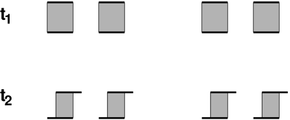
Figure 1: The overlap of two identical Cantor sets of dimension $\ln 2/\ln 3$ at generation $n=2$ as one moves over the other with uniform velocity. The total measure $O$ of the overlap (total shaded region) varies with time and are shown for two different time instances.

Since the index of the central term (i.e., the term for the most probable event) of the above distribution is $n/3+\delta$, $-2/3<\delta<1/3$, for large values of $n$ Eq. (3) may be written as

$$F\left({n\over 3}\pm r\right)\approx\left(\begin{array}[]{c}n\\ n\pm r\end{array}\right)\left({1\over 3}\right)^{{n\over 3}\pm r}\left({2\over 3}\right)^{{2n\over 3}\mp r}$$ (4)

by replacing $n-k$ with $n/3\pm r$. For $r\ll n$, we can write the normal approximation to the above binomial distribution as

$$F\left({n\over 3}\pm r\right)\sim{3\over\sqrt{2\pi n}}\exp{\left(-{9r^{2}\over 2n}\right)}$$ (5)

Since $\log_{2}O=n-k={n\over 3}\pm r$, we have

$$F\left(\log_{2}O\right)\sim{1\over\sqrt{n}}\exp{\left[-{\left(\log_{2}O\right)^{2}\over n}\right]},$$ (6)

not mentioning the factors that do not depend on $O$. Now

$$F\left(\log_{2}O\right)\mathrm{d}\left(\log_{2}O\right)\equiv G(O)\mathrm{d}O$$ (7)

where

$$G(O)\sim{1\over O}\exp\left[-{\left(\log_{2}O\right)^{2}\over n}\right]$$ (8)

is the log-normal distribution of $O$. As the generation index $n\to\infty$, the normal factor spreads indefinitely (since its width is proportional to $\sqrt{n}$) and becomes a very weak function of $O$ so that it may be considered to be almost constant; thus $G(O)$ asymptotically assumes the form of a simple power law with an exponent that is independent of the fractal dimension of the overlapping Cantor sets CCB:Bhattacharyya:2006 :

$$G(O)\sim{1\over O}\ \mathrm{for}\ n\to\infty.$$ (9)

III The Cantor set overlap time series

Figure 2: (a) The time series data of overlap size $O(t)$ for a regular Cantor set of dimension $\rm{ln}4/\rm{ln}5$ at generation $n=4$. (b) Cumulative overlap $Q^{o}(t)$ and (c) the variation of the cumulative overlap $Q^{o}_{i}(t)$ for the same series, where $Q$ is reset to zero after any big event of size greater than $\Delta=150$.

We now consider the time series $O(t)$ of the overlap set (of two identical fractals CCB:Pradhan:2004 ; CCB:Bhattacharyya:2005 ), as one slides over the other with uniform velocity. Let us again consider two regular cantor sets at finite generation $n$. As one set slides over the other, the overlap set changes. The total overlap $O(t)$ at any instant $t$ changes with time (see Fig. 2(a)). In Fig. 2(b) we show the behavior of the cumulative overlap CCB:Pradhan:2004 $Q^{o}(t)=\int_{0}^{t}O(\tilde{t})d\tilde{t}$. This curve, for sets with generation $n=4$, is approximately a straight line CCB:Pradhan:2004 with slope $(16/5)^{4}$. In general, this curve approaches a strict straight line in the limit $a\rightarrow\infty$, asymptotically, where the overlap set comes from the Cantor sets formed of $a-1$ blocks, taking away the central block, giving dimension of the Cantor sets equal to $\mathrm{ln}(a-1)/\mathrm{ln}a$. The cumulative curve is then almost a straight line and has then a slope $\left[(a-1)^{2}/a\right]^{n}$ for sets of generation $n$. If one defines a ‘crash’ occurring at time $t_{i}$ when $O(t_{i})-O(t_{i+1})\geq\Delta$ (a preassigned large value) and one redefines the zero of the scale at each $t_{i}$, then the behavior of the cumulative overlap $Q^{o}_{i}(t)=\int_{t_{i-1}}^{t}O(\tilde{t})d\tilde{t},\;\tilde{t}\leq t_{i}$, has got the peak value ‘quantization’ as shown in Fig. 2(c). The reason is obvious. This justifies the simple thumb rule: one can simply count the cumulative $Q^{o}_{i}(t)$ of the overlaps since the last ‘crash’ or ‘shock’ at $t_{i-1}$ and if the value exceeds the minimum value ($q_{o}$), one can safely extrapolate linearly and expect growth upto $\alpha q_{o}$ here and face a ‘crash’ or overlap greater than $\Delta$ ($=150$ in Fig. 2). If nothing happens there, one can again wait upto a time until which the cumulative grows upto $\alpha^{2}q_{o}$ and feel a ‘crash’ and so on ($\alpha=5$ in the set considered in Fig. 2).

IV The stock price time series

Figure 3: Data from New York Stock Exchange from January 1966 to December 1979: industrial index CCB:NYSE : (a) Daily closing index $S(t)$ (b) integrated $Q^{s}(t)$, (c) daily changes $\delta S(t)$ of the index $S(t)$ defined as $\delta S(t)=S(t+1)-S(t)$, and (d) behavior of $Q_{i}^{s}(t)$ where $\delta S(t_{i})>\Delta$. Here, $\Delta=-1.0$ as shown in (c) by the dotted line (from CCB:PFE ).

Figure 4: Data from New York Stock Exchange from January 1966 to December 1979: utility index CCB:NYSE : (a) Daily closing index $S(t)$ (b) integrated $Q^{s}(t)$, (c) daily changes $\delta S(t)$ of the index $S(t)$ defined as $\delta S(t)=S(t+1)-S(t)$, and (d) behavior of $Q_{i}^{s}(t)$ where $\delta S(t_{i})>\Delta$. Here, $\Delta=-0.530$ as shown in (c) by the dotted line.

We now consider some typical stock price time-series data, available in the internet. The data analyzed here are for the New York Stock Exchange (NYSE) Indices CCB:NYSE . In Fig. 3(a), we show that the daily stock price $S(t)$ variations for about $10$ years (daily closing price of the ‘industrial index’) from January 1966 to December 1979 (3505 trading days). The cumulative $Q^{s}(t)=\int_{0}^{t}S(t)dt$ has again a straight line variation with time $t$ (Fig. 3(b)). Similar to the Cantor set analogy, we then define the major shock by identifying those variations when $\delta S(t)$ of the prices in successive days exceeded a preassigned value $\Delta$ (Fig. 3(c)). The variation of $Q_{i}^{s}(t)=\int_{t_{i-1}}^{t_{i}}S(\tilde{t})d\tilde{t}$ where $t_{i}$ are the times when $\delta S(t_{i})\leq-1$ show similar geometric series like peak values (see Fig. 3(d)); see CCB:PFE .

We observed striking similarity between the ‘crash’ patterns in the Cantor set overlap model and that derived from the data set of the stock market index. For both cases, the magnitude of crashes follow a similar pattern — the crahes occur in a geometric series.

A simple ‘anticipation strategy’ for some of the crashes may be as follows: If the cumulative $Q_{i}^{s}(t)$ since the last crash has grown beyond $q_{0}\simeq 8000$ here, wait until it grows (linearly with time) until about $17,500$ ($\simeq 2.2q_{0}$) and expect a crash there. If nothing happens, then wait until $Q_{i}^{s}(t)$ grows (again linearly with time) to a value of the order of $39,000$ ($\simeq(2.2)^{2}q_{0}$) and expect a crash, and so on.

The same kind of analysis for the NYSE ‘utility index’, for the same period, is shown in Figs. 4.

V Earthquake magnitude time series

Unlike in the case of stock price time series where accurate data are easily available, the time series for earthquake magnitudes $M(t)$ at any fault involves considerably coordinated measurements and comparable accuracies are not easily achievable. Still from the available data, as in the case of stock market (where the integrated stock price $Q^{s}(t)$ shows clear linear variations with time and this fits well with that for the cumulative overlap $Q^{o}(t)$ for the fractal overlap model; see also CCB:EQbook ), the integrated earthquake magnitude $Q^{m}(t)=\int_{0}^{t}M(t)dt$ of the aftershocks does also show such prominent linear variations (see Fig. 5). We believe, the slopes of these linear $Q^{m}(t)$ vs. $t$ curves for different faults would give us the signature of the corresponding fractal structure of the underlying fault. It may be noted in this context, in our model, the slope becomes $[(a-1)^{2}/a]^{n}$ for an $n$th generation Cantor set, formed out of the remaining $a-1$ blocks having the central block removed.

Figure 5: Local earthquake data from US geological Survey Southern California catalogs. CCB:USGS : Top: Time series of successive quakes $M(t)$; Bottom: integrated $Q^{m}(t)$. The dataset is a record of quakes between 1 January 2003 to 31 March 2004, between depths 0 and 700 kms, between latitudes 32 N and 37 N and longitudes -122 W and -114 W.

VI Summary

Based on the formal similarity between the two-fractal overlap model of earthquake time series and of the stock market, we considered here a detailed comparison. We find, the features of the time series for the overlap of two Cantor sets when one set moves with uniform relative velocity over the other looks somewhat similar to the time series of stock prices. We analyze both and explore the possibilities of anticipating a large (change in Cantor set) overlap or a large change in stock price. An anticipation method for some of the crashes has been proposed here, based on these observations.

References

- (1) Sornette D (2003) Why Stock Markets Crash? Princeton Univ. Press, Princeton; Mantegna RN, Stanley HE (1999) Introduction to Econophysics. Cambridge Univ. Press, Cambridge
- (2) Chakrabarti BK, Stinchcombe RB (1999) Physica A 270:27-34
- (3) Pradhan S, Chakrabarti BK, Ray P, Dey MK (2003) Phys. Scr. T106:77-81
- (4) Pradhan S, Chaudhuri P, Chakrabarti BK (2004) in Continuum Models and Discrete Systems, Ed. Bergman DJ, Inan E, Nato Sc. Series, Kluwer Academic Publishers, Dordrecht, pp.245-250; cond-mat/0307735
- (5) Bhattacharyya P (2005) Physica A 348:199-215
- (6) Bhattacharyya P, Chatterjee A, Chakrabarti BK (2007) Physica A, 381:377-382
- (7) NYSE Daily Index Closes from http://www.unifr.ch/econophysics
- (8) Chakrabarti BK, Chatterjee A, Bhattacharyya P (2006) in Takayasu H (Ed) Practical Fruits of Econophysics, Springer, Tokyo, pp. 107-110; arxiv:physics/0510047.
- (9) Bhattacharyya P, Chakrabarti BK (Eds) (2006) Modelling Critical and Catastrophic Phenomena in Geoscience, Lecture Notes in Physics, vol. 705, Springer-Verlag, Heidelberg
- (10) U S Geological Survey, Southern California Catalogs, www.data.scec.org.