Strong tunable coupling between a superconducting charge and phase qubit

Abstract

We have realized a tunable coupling over a large frequency range between an asymmetric Cooper pair transistor (charge qubit) and a dc SQUID (phase qubit). Our circuit enables the independent manipulation of the quantum states of each qubit as well as their entanglement. The measurements of the charge qubit’s quantum states is performed by resonant read-out via the measurement of the quantum states of the SQUID. The measured coupling strength is in agreement with an analytic theory including a capacitive and a tunable Josephson coupling between the two qubits.

Interaction between two quantum systems induces entangled states whose properties have been studied since the 80’s for pairs of photons Dalibard_PRL82 , for atoms coupled to photons Raimond_RMP01 and for trapped interacting ionsLeibfried_RMP03 . In the last decade, quantum experiments were extended to macroscopic solid state devices opening the road for application within the field of quantum information. In superconducting circuits, theoretical proposals Buisson_00 ; Plastina_PRB03 ; Blais_PRA04 and experimental realizations on interacting quantum systems were put forward. In these systems coupling has been achieved between a quantum two-level system (qubit) and a resonatorChiorescu_Nature04 ; Wallraff_Nature04 ; Johansson_PRL06 as well as between two identical qubitsPashkin_Nature03 ; Berkley_Science03 ; McDermott_Science05 . In these pioneering circuits the interaction between the quantum systems was realized through a fixed capacitive or inductive coupling. The tunability of the coupling strength appears as an important issue to optimize the control of two or more coupled quantum systems. Indeed it enables to decouple the quantum systems for individual manipulations and to couple them when entanglement between the quantum states is needed. Recently different tunable couplings between two identical qubits have been proposed and measuredAverin_PRL03 ; Niskanen_Science07 ; Hime_Science06 ; Sillanpaa_Science07 ; Majer_Nature07 . In this Letter we report for the first time on a tunable composite coupling between a charge qubit, an asymmetric Cooper pair transistor (ACPT) and a phase qubit, a dc SQUID. In our circuit (see Fig.1) the coupling is composed of two independent terms, a fixed capacitive and a tunable Josephson part, leading to a tunability of the total coupling.

The dynamics of the current biased dc SQUID can be described by the Hamiltonian of an anharmonic oscillator: $\hat{H}_{S}=\frac{1}{2}h\nu_{p}(\hat{P}^{2}+\hat{X}^{2})-\sigma h\nu_{\rm p}\hat{X}^{3}$ where $\nu_{p}$ is the plasma frequency of the SQUID. Here $\hat{P}$ and $\hat{X}$ are the reduced charge and phase conjugate operatorsClaudon_PRL04 . In our case the anharmonicity prevents multi-plasmon excitation and therefore the system at low energy reduces to a two-level system with levels denoted by $|0\rangle$ and $|1\rangle$ corresponding respectively to the zero- and one-plasmon state. At low energies the SQUID Hamiltonian therefore reads $\hat{H}_{S}=h\nu_{S}\hat{\sigma}_{z}^{S}\,/2$ where $\hat{\sigma_{z}}$ is the Pauli matrix. The frequency between these two levels $\nu_{S}$ depends on the working point and is determined by the dc flux $\Phi_{S}$ through the SQUID loop and the bias current $I_{b}$. The ACPT can be described as a two-level system with quantum states denoted by $|-\rangle$ and $|+\rangle$ for respectively the ground and first excited state. The hamiltonian of the ACPT takes the form $\hat{H}_{T}=h\nu_{T}\hat{\sigma}_{z}^{T}\,/2$ where $\nu_{T}$ depends on the gate-induced charge $n_{g}$ and the phase difference $\delta$ across the transistor. We now turn to the coupling of both quantum systems in a circuit shown in Fig.1. As the ACPT is in parallel to the SQUID, both a Josephson and a capacitive coupling appear between these two quantum systems. The Josephson coupling results from the phase relation along the loop between the transistor bias and the closer SQUID junction. The capacitive coupling is explained by the charge displacement between the transistor and SQUID capacitance. The total coupling can be tuned in our circuit from about $1.2GHz$ down to $0.1GHz$.

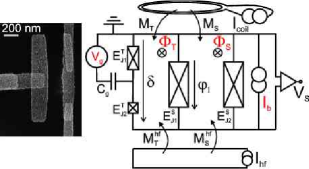
Figure 1: Electrical schematic of the coupled circuit. The working point is controlled by a dc gate voltage $V_{g}$, a current biased $I_{b}$ and the fluxes $\Phi_{T}$ and $\Phi_{S}$. The current $I_{coil}$ and $I_{hf}$ produces a flux on the SQUID and transistor through respectively the mutual $M_{S}$, $M_{T}$ and $M_{S}^{hf}$, $M_{T}^{hf}$. The high frequency (hf) line is also used to produce a $\mu$w flux pulse and a nanosecond flux pulse for the escape measurement of the SQUID. On the left side a SEM image of the asymmetry Cooper pair transistor.

.

The ACPT consists of a superconducting island connected by two Josephson junctions of different surfaces of about $0.02\ \mu$m² and $0.05\ \mu$m², respectively to the supercondcuting electrodes. The dc SQUID comprises two large Josephson junctions of $5\ \mu$m² area each, enclosing a $347\ \mu$m² superconducting loop. The ACTP and the SQUID Josephson junction closer to the ACPT realizes a second loop of $126\ \mu$m² surface. The coupled circuit is realized by a three angle shadow evaporation of aluminum with two different oxydations respectively for the SQUID junctions and the ACPT junctions. Measurements are performed in a dilution fridge at $T=30\>\text{mK}$. The microwave ($\mu$w) flux and charge-gate signal are guided by $50\>\Omega$ coax lines and $40dB$ attenuated at low temperature before reaching the circuit through a mutual inductance and the gate capacitance, respectively. The measurement of the quantum states of the circuits is performed by a nanosecond flux pulse which produces switching to the voltage state of the SQUIDClaudon_PRB07 .

We first study the individual resonant frequency of the SQUID and the ACPT (Fig. 2). Spectroscopy measurements of the SQUID are performed by a $\mu$w flux pulse followed by a nanosecond flux pulse. The escape probability shows a resonant peak associated with the transition $|0\rangle\rightarrow|1\rangle$ (inset (a) of Fig. 2). The SQUID resonance frequency $\nu_{S}$ can be tuned from 8GHz to more than 20GHz as a function of the bias current $I_{b}$ and the magnetic flux $\Phi_{S}$ in the SQUID loop. ¿From flux calibration, we obtain $M_{S}=0.13$ pH and $M_{S}^{hf}=1.58$ pH. From the measured resonance frequency $\nu_{S}$ the SQUID parameters such as $E_{J}^{S}$, $E_{C}^{S}$ and the total SQUID inductance $L$ can be determined with a precision better than $1\%$. We find a critical current of $I^{S}_{c}=1346nA$, a capacitance $C^{S}=0.227pF$ per junction, an inductance $L=190pH$ and an inductance asymmetry of $\eta=0.29$ between the two SQUID arms. These values are similar to typical parameters of previous samplesClaudon_PRB07 . When the SQUID’s working point frequency increases from 8GHz to 20GHz the resonance width changes from 200MHz to 20MHz. The finite width is consistent with a 10nA RMS current noise and a $1m\Phi_{0}$ RMS flux noiseClaudon_PRB06 . Rabi-like oscillations have been measured with a typical decay time of about 10ns and a relaxation time of about 30ns. These times are shorter in comparison to our previous SQUID sample. Moreover a high density of parasitic resonances is observed in the current sample (see Fig. 9 of Ref. Claudon_PRB07 ) which could explain these shorter times. The origin of these resonances is still not completely understood but has been already observed in other phase-qubits Cooper_PRL04 . All presented measurements have been done at working points where these parasitic resonances are not visible through spectroscopy measurements.

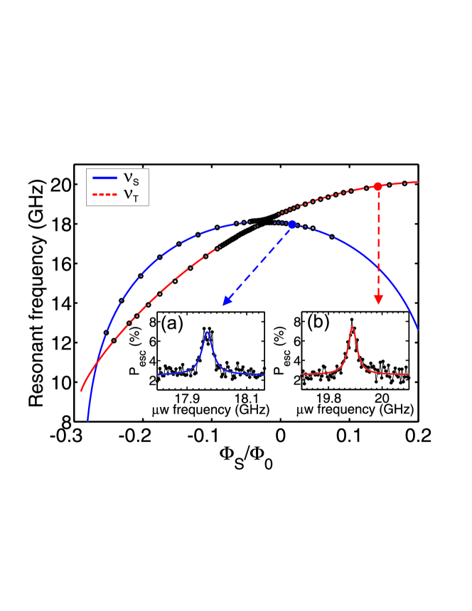
Figure 2: Experimental resonant frequency versus $\Phi_{S}$ for the coupled circuit with $I_{b}=1890$ nA and $n_{g}=1/2$. The blue and red solid lines are the fit using the uncoupled hamiltonians of the dc SQUID and the ACPT respectively. Inset: Escape probability of the SQUID versus frequency probing (a) the SQUID at $\Phi_{S}=0.02\ \Phi_{0}$ and (b) the ACPT at $\Phi_{S}=0.14\ \Phi_{0}$ (fitted by a lorentzian law).

The energy levels of the ACPT can be determined as well by escape probability measurements on the SQUID via resonant read out. We apply a $\mu$w signal of 1$\mu$s on the gate line at fixed frequency when the ACPT and the SQUID are off resonance. If the applied $\mu$w frequency matches the ACPT frequency the $|+\rangle$ level of the ACPT is populated. For the measurement a nanosecond flux pulse with a rise time of 2 ns drives the two systems adiabatically across the resonance where the coupling is about 1 GHz (see below). The initial state $|+,0\rangle$ is thereby transferred into the state $|-,1\rangle$ Buisson_PRL03 . Afterwards an escape measurement is performed on the SQUID (Inset b of Fig.2).

The ACPT resonant frequency as a function of $\delta$ at $n_{g}=1/2$ is shown in Fig. 3. Here $\delta$ is given by the relation $\delta=\varphi_{1}+L_{1}\,I_{c}^{S}sin(\varphi_{1})/\Phi_{0}-2\pi\Phi_{T}/\Phi_{0}$ where is $\Phi_{T}$ the dc flux inside the loop, $\phi_{1}$ the phase difference across the SQUID junction closer to the transistor and $L_{1}$ the inductance of the corresponding branch of the SQUID. In our set-up we have $M_{T}=0.047$ pH and $M_{T}^{hf}=0.35$ pH and $L_{1}=70$ pH. The qubit resonant frequency $\nu_{T}$ versus $\delta$ can be fitted within $1\%$ error by considering that the $|+\rangle$ and $|-\rangle$ states are superpositions of four charge states. The ACPT has two optimal working points for qubit manipulations. The one at ($n_{g},\delta$)=(1/2,0) was extensively studied in the Quantronium symmetric transistorVion_Science02 . The ($n_{g},\delta$)=(1/2,$\pi$) working point appears as a new optimal point created by the asymmetry of the transistor. The width of the resonance peak far from the optimal points is typically $40$ MHz while close to the two optimal points $\delta=0$ and $\delta=\pi$, it is typically around 20MHz. From the two extreme resonant frequencies $\nu_{T}=20.302$ GHz and $\nu_{T}=8.745$ GHz, the critical current of the two junctions can be deduced and we obtain $I^{T}_{c,1}=30.1nA$ and $I^{T}_{c,2}=12.3nA$. From the frequency spectrum $\nu_{T}$ versus the gate charge $n_{g}$, we find a total transistor capacitance of $C^{T}=2.9fF$ and a gate capacitance $C_{g}=29aF$. Fig.3a presents Rabi oscillations in the ACPT at the new optimal point ($n_{g},\delta$)=(1/2,$\pi$). The Rabi frequency follows a linear dependance on the $\mu$w amplitude as expected for a two-level quantum system. The two level system presents a long relaxation time of about $800ns$ (Fig. 3b).

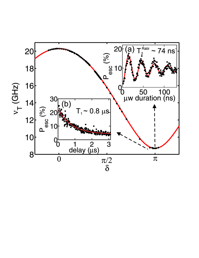
Figure 3: The ACPT energy versus $\delta$ at $n_{g}=0.5$ fitted by the ACPT hamiltonian. Inserts: Measurements at $\delta=\pi$. (a) Escape probability versus $\mu$w pulse duration for $-3dBm$ room temperature $\mu$w power. (b) Escape probability versus delay time between the $\mu$w and the measurement pulse fitted by an exponential decay (continuous line) giving $T_{1}=810ns$.

Hereafter we consider the case when the two qubits are in resonance ($\nu_{T}=\nu_{S}$). Fig. 4a shows the measured escape probability at the working point $I_{b}=1647$ nA and $\Phi_{S}=0.03\ \Phi_{0}$ for two different gate charges $n_{g}=1/2$ and $n_{g}\sim 1$ corresponding respectively to the in and off resonance case. Off resonance, the ACPT frequency being very much larger than the SQUID resonance, only one resonance peak is observed which corresponds to the $|1\rangle$ state excitation of the SQUID. At $n_{g}=1/2$ the resonance condition between the ACPT and the SQUID is satisfied for this working point. The coupling between the two systems leads to a splitting of the resonance peak of about $120$ MHz into two peaks corresponding to the two entangled states $|0,+\rangle\pm|1,-\rangle$. The resonance width is about four times thinner than the coupling strength which demonstrates clearly the strong coupling of the ACPT two-level system with the zero- and the one-plasmon state of the dc SQUID. In Fig. 4b, the escape probability versus $n_{g}$ and $\mu$w frequency is plotted at the same working point. Far from the resonance condition the value can be well estimated assuming two uncoupled circuits. In the vicinity of $n_{g}=1/2$, anti-level crossing occurs modifying the individual resonance frequency of the two circuits. In Fig. 4c, the escape probability versus $\Phi_{S}$ and $\mu$w frequency is measured at $n_{g}=1/2$ at a different working point. Anti-level crossing is clearly observed with a splitting of about $900$MHz. The width of the two resonances strongly depends on $\Phi_{S}$ and varies from $200$MHz to about $40$MHz as the crossing point is passed. This effect can be explained by the large difference of the resonance width of the SQUID and the ACPT around this working point.

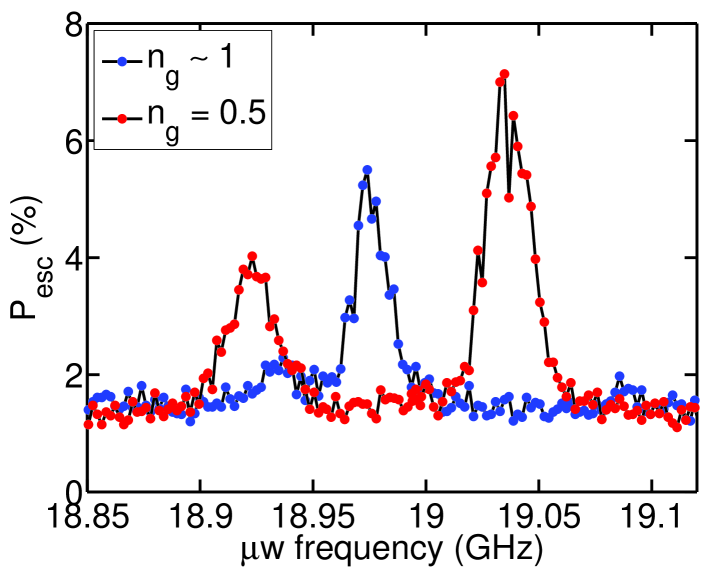
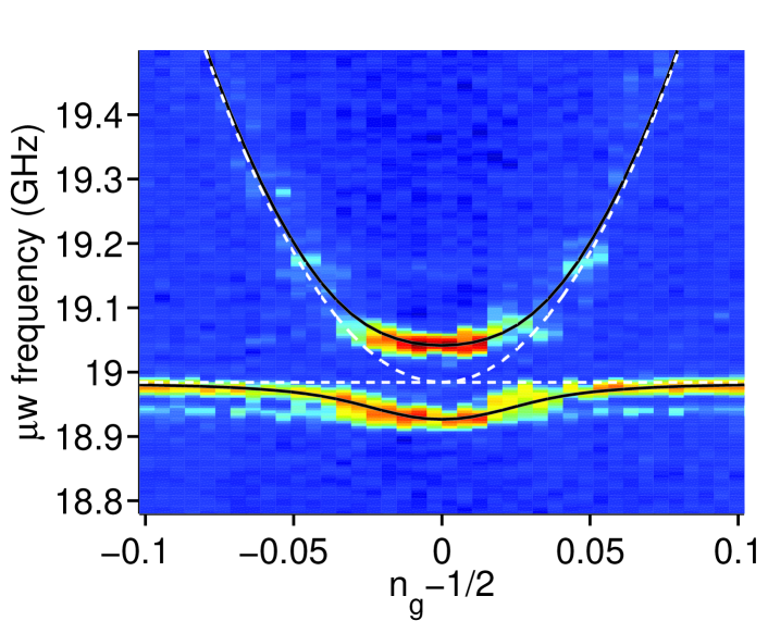
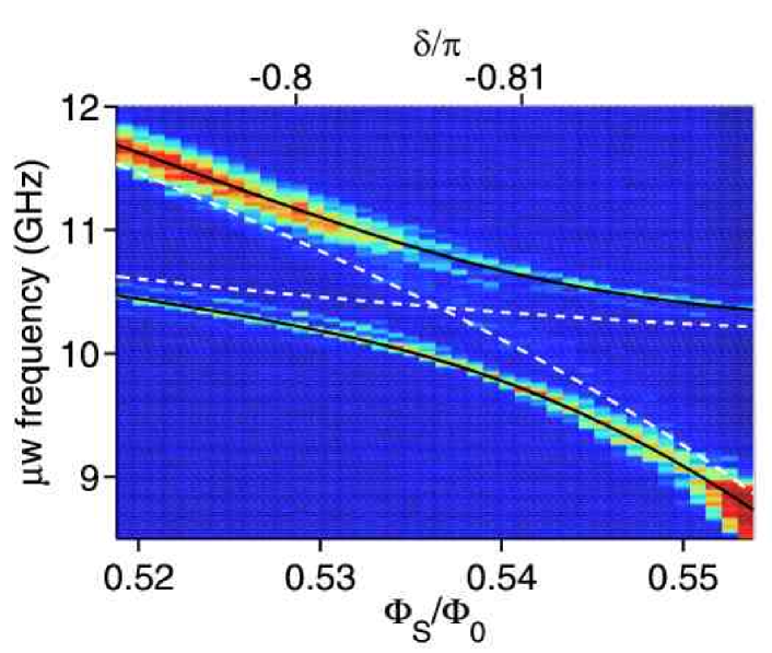
Figure 4: (a)Escape probability of the SQUID at the working point $I_{b}=1647$ nA, $\Phi_{S}=0.03\ \Phi_{0}$, $\delta=0.26\pi$. Blue curve: At $n_{g}\sim 1$ SQUID and ACPT are out off resonance ($\nu_{T}\sim 31.6$ GHz). Red curve: At $n_{g}=0.5$ the resonance condition is fulfilled leading to antilevel-crossing.(b) $P_{esc}$ versus $n_{g}$ and $\mu$w frequency at the working point $I_{b}=1647$ nA, $\Phi_{S}=0.03\ \Phi_{0}$ and $\delta=0.26\pi$. ( c) $P_{esc}$ versus $\Phi_{S}$($\delta$) and $\mu$w frequency at the working point $I_{b}=107$ nA and $n_{g}=1/2$. Blue color corresponds to small $P_{esc}$ , red color to large $P_{esc}$. Dashed and continuous lines correspond to uncoupled and coupled cases.

The coupling strength between the two qubits is measured at $n_{g}=1/2$ and at the working points where the resonance condition $\nu_{T}=\nu_{S}$ is satisfied. The frequency splitting is plotted versus the resonant frequency in Fig.5. The coupling is minimal at $\nu_{T}=20.3GHz$ and strongly increases with decreasing resonant frequency up to a maximum value of 1.2 GHz. Note that when the resonance frequency changes from 20.3 GHz down to 8.8 GHz the phase bias over the ACPT changes from $\delta=0$ to $\delta=\pi$. We find therefore nearly zero coupling at $\delta=0$ and a very strong coupling of 1.2 GHz at $\delta=\pi$.

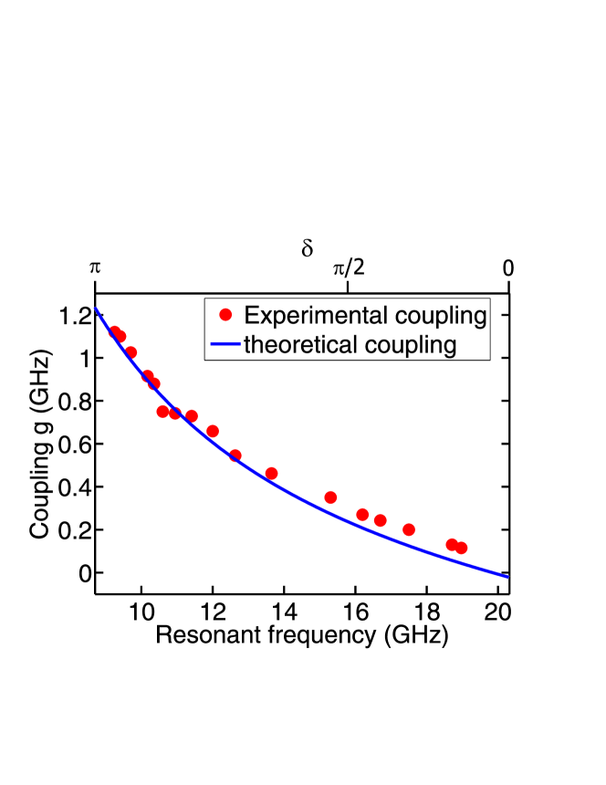
Figure 5: Coupling strength versus the frequency at the resonance condition between the two circuits at $n_{g}=1/2$. The points are experimental data and the continuous line is the theoretical prediction.

For the theoretical analysis we consider that the transistor $|-\rangle$ and $|+\rangle$ states are superpositions of two charge states and we neglect anharmonicity effects of the SQUID potential on the frequency $\nu_{S}$. We obtain the following analytical expression for the coupling strength at a gate charge of $n_{g}=1/2$: $H_{coupling}=(E_{c,c}/4)\sigma_{S}^{x}\sigma_{T}^{x}-E_{c,j}/2(\cos(\chi-\delta/2)\sigma_{S}^{y}\sigma_{T}^{y}+\sin(\chi-\delta/2)\sigma_{S}^{y}\sigma_{T}^{z}/2)$, where $E_{c,c}=(1-\lambda)\sqrt{E_{C}^{S}/h\nu_{p}}h\nu_{p}$ and $E_{c,j}=(1-\mu)\sqrt{E_{C}^{S}/h\nu_{p}}E^{T}_{j}$ with $\lambda=(C^{T}_{1}-C^{T}_{2})/(C^{T}_{1}+C^{T}_{2})$ and $\mu=(E^{T}_{J,1}-E^{T}_{J,2})/(E^{T}_{J,1}+E^{T}_{J,2}$) being the transistor capacitance and Josephson energy asymmetry, respectively. $E_{C}^{S}\approx e^{2}/2C^{S}$ with $C^{S}$ the SQUID capacitance, $E^{T}_{j}=E^{T}_{J,1}+E^{T}_{J,2}$ the transistor Josephson energy and $\tan(\chi)=-\mu\,\tan(\delta/2)$. The coupling contains two independent contributions: one related to the capacitance and the other one to the Josephson coupling of the ACPT. Close to resonance, slow dynamics dominates and the hamiltonian simplifies to a Jaynes-Cummings type Hamiltonian $H_{coupling}=\frac{1}{2}g(\sigma_{S}^{+}\sigma_{T}^{-}+\sigma_{S}^{-}\sigma_{T}^{+})$ where $g=(E_{c,c}/2-E_{c,j}\cos(\chi-\delta/2))$ and $\sigma_{S/T}^{+/-}$ creates or annihilates an excitation in the SQUID or the ACPT. At this point we stress that the coupling strength at $n_{g}=1/2$ depends only on the $\delta$ parameter. If we replace one of the transistor junctions by a pure capacitance ($E^{T}_{J,2}=0$) we obtain $E_{c,j}=0$ and we retrieve the capacitive coupling Buisson_00 calculated for a Cooper pair box coupled to a SQUID. For a symmetric transistor ($\lambda=\mu=0$) the charge and the Josephson coupling compensate each other, giving zero coupling for any value of the $\delta$ parameter. It is the asymmetry of the transistor which enables non zero coupling at the optimum point of the charge qubit. In particular, for the case that $\lambda=\mu$ - which is realized for a transistor containing two junctions having the same plasma frequency - the total coupling vanishes at $\delta=0$ but becomes non zero at the second optimum point at $\delta=\pi$. By assuming an asymmetry of $\mu=\lambda=41.9\%$ for our sample the coupling strength can be very well fitted without any other free parameters as can be seen in Fig. 5. The slight discrepancy can be explained by a small difference between $\lambda$ and $\mu$.

In conclusion, we have demonstrated strong tunable coupling between two superconducting qubits. Far from resonance our quantum circuit enables us to control the quantum dynamics of each qubit separately. At resonance we demonstrate entanglement between the quantum states of the charge and phase qubit which is consistent with the exchange of a single energy quantum. The measured coupling strength could be perfectly understood by an analytical coupling expression of the type Jaynes-Cumings Hamiltonian. The quantum state measurement of the charge-phase qubit has been performed via resonant readout by measuring the quantum state of the SQUID. Our result encourages the future development of quantum information processing in solid-state devices.

We thank for fruitful discussions. This work was supported by two ACI programs, by the EuroSQIP project and by the Institut de Physique de la Matière Condensée.

References

- (1) A. Aspect, J. Dalibard, G. Roger, Phys. Rev. Let. 49, 1804 (1982).
- (2) J. Raimond, M. Brune, and S. Haroche, Rev. Mod. Phys. 73, 565 (2001).
- (3) D. Leibfried, R. Blatt, C. Monroe, D. Wineland, Rev. Mod. Phys. 75, 565 (2003).
- (4) O. Buisson and F. W. J. Hekking, in Macroscopic quantum coherence and computing, p. 137, edited by D. Averin, B. Ruggiero, and P. Silvestrini (Kluwer Academic, New York, 2001).
- (5) F. Plastina and G. Falci, Phys. Rev. B67 224514 (2003)
- (6) A. Blais, R.-S. Huang, A. Wallraff, S. M. Girvin, and R. J. Schoelkopf, Phys. Rev. A 69, 062320 (2004).
- (7) I. Chiorescu, P. Bertet, K. Semba, Y. Nakamura, C. J. P. M. Harmans, and J. E. Mooij, Nature 431, 162 (2004);
- (8) A. Wallraff, D. I. Schuster, A. Blais, L. Frunzio, R.-S. Huang, J. Majer, S. Kumar, S. M. Girvin, and R. J. Schoelkopf, Nature 431, 162 (2004).
- (9) J. Johansson, S. Saito, T. Meno, H. Nakano, M. Ueda, K. Semba, H. Takayanagi , Phys. Rev. Lett. 96, 127006 (2006).
- (10) Yu. A. Pashkin, T. Yamamoto, O. Astafiev, Y. Nakamura, D. V. Averin, and J. S. Tsai, Nature 421, 823 (2003)
- (11) A. J. Berkley, H. Xu, R. C. Ramos, M. A. Gubrud, F. W. Strauch, P. R. Johnson, J. R. Anderson, A. J. Dragt, C. J. Lobb, and F. C. Wellstood, Science 300, 1548 (2003).
- (12) R. McDermott, R. W. Simmonds, M. Steffen, K. B. Cooper, K. Cicak, K. D. Osborn, S. Oh, D. P. Pappas, and J. M. Martinis, Science 307, 1299 (2005).
- (13) D. V. Averin and C. Bruder, Phys. Rev. Lett. 91, 057003 (2003).
- (14) A.O. Niskanen, K. Harrabi, F. Yoshihara, Y. Nakamura, S. Lloyd, and J. S. Tsai, Science 316, 723 (2007).
- (15) T. Hime, P.A. Reichardt, B. L. T. Plourde, T. L. Robertson, C.E Wu, A. V. Ustinov, J. Clarke, Science 314, 1427 (2006).
- (16) M. Sillanpaa, J. I. Park, R. W. Simmonds, Nature 449, 438 (2007).
- (17) J. Majer, J. M. Chow, J. M. Gambetta, Jens Koch, B. R. Johnson, J. A. Schreier, L. Frunzio, D. I. Schuster, A. A. Houck, A. Wallraff, A. Blais, M. H. Devoret, S. M. Girvin and R. J. Schoelkopf. Nature 449, 443 (2007).
- (18) D. Vion D, A. Aassime, A. Cottet, P. Joyez, H. Pothier, C. Urbina, D. Esteve, and M. H. Devoret, Science 296, 886 (2002);
- (19) J. Claudon, F. Balestro, F.W. J. Hekking, and O. Buisson, Phys. Rev. Lett. 93, 187003 (2004).
- (20) J. Claudon, A. Fay, E. Hoskinson, and O. Buisson, Phys. Rev. B 76, 024508 (2007).
- (21) J. Claudon, A. Fay, L.P. Lévy and O. Buisson, Phys. Rev. B 73, 180502 (2007).
- (22) K. B. Cooper, M. Steffeen, R. McDermott, R. W. Simmonds, S. Oh, D. A. Hite, D. P. Pappas, and J. M. Martinis, Phys. Rev. Lett. 93, 180401 (2004).
- (23) O. Buisson, F. Balestro, J. P. Pekola, and F. W. J. Hekking, Phys. Rev. Lett. 90, 238304 (2003).