Shear viscosity of liquid helium 4 above the $\lambda$ point

Abstract

In liquid helium 4, many features associated to Bose statistics have been masked by the strongly interacting nature of the liquid. As an example of these features, we examine the shear viscosity of liquid helium 4 above the $\lambda$ point. Applying the linear-response theory to Poiseuille’s formula for the capillary flow, the reciprocal of the shear viscosity coefficient $\eta$ is considered as a transport coefficient. Using the Kramers-Kronig relation, we relate a superfluid flow in a capillary with that in a rotating bucket, and express $1/\eta$ in terms of the susceptibility of the system. A formula for the kinematic shear viscosity $\nu$ is obtained which describes the influence of Bose statistics. Using this formula, we study the gradual fall of $\nu(T)$ from $3.7K$ to $T_{\lambda}$ in liquid helium 4 at 1 atm.

I Introduction

The shear viscosity of liquid helium 4 has been subjected to considerable experimental and theoretical studies. Well below the lambda temperature $T_{\lambda}$, various excitations of a liquid are strictly suppressed except for phonons and rotons. Hence, it is natural to assume that they are responsible for the shear viscosity appearing in the damping of an oscillating disc, or the drag of a rotating cylinder at $T<T_{\lambda}$. By regarding these phonons and rotons as a weakly interacting dilute Bose gas, the kinetic theory of gases properly describes the shear viscosity of liquid helium 4 at $T\ll T_{\lambda}$ kha .

For the shear viscosity above $T_{\lambda}$, however, the dilute-gas picture must not be applied, because the macroscopic condensate, which is the basis for the above picture, has not yet developed. Rather, we must deal with the influence of Bose statistics on the dissipation mechanism of a liquid. In an ordinary liquid flowing along x-direction, the shear viscosity causes the shear stress $F_{xy}$ between two adjacent layers at different velocities

$$F_{xy}=\eta\frac{\partial v_{x}}{\partial y},$$ (1)

where $\eta$ is the coefficient of shear viscosity. In the linear response theory, $\eta$ of a stationary flow is given by the following two-time correlation function of a tensor $J_{xy}(t)=-\sum_{i}(p_{i,x}p_{i,y}/m)$

$$\eta=\frac{1}{Vk_{B}T}\int_{0}^{\infty}dt<J_{xy}(0)J_{xy}(t)>.$$ (2)

In principle, $\eta$ of a liquid, and therefore the effect of Bose statistics on $\eta$ is obtained by calculating an infinite series of the perturbation expansion of Eq.(2) with respect to the particle interaction $U$ kad . At first sight, however, it seems to be a hopeless attempt, because the dissipation in a liquid is a complicated phenomenon allowing no simple explanation han jeo . In liquid helium 4, many features associated to Bose statistics have been masked by the strongly interacting nature of the liquid.

In this paper, we will go back to the original phenomenon which has been known from 1938. Superfluidity was first discovered in a flow through a channel and a flow through a capillary kap . In an ordinary flow through a capillary (a radius $a$ and a length $L$), the velocity distribution under the pressure difference $\Delta P$ has a form such as

$$v_{z}(r)=\frac{a^{2}-r^{2}}{4\eta}\frac{\Delta P}{L},$$ (3)

where $r$ is a radius in the cylindrical coordinates (Poiseuille flow. Fig.1). In the superfluid phase of liquid helium 4, even when the pressure difference vanishes ($\Delta P=0$), one observes a non-vanishing flow ($v_{z}(r)\neq 0$), hence $\eta=0$ in Eq.(3). Instead of Eq.(2), we will regard Poiseuille’s formula Eq.(3) as a linear-response relation. Without loss of generality, we may focus on a flow velocity at a single point, for example, $\mbox{\boldmath$v$}(r=0)$ on the axis of rotational symmetry (z-axis). We define a mass flow density $\mbox{\boldmath$j$}=\rho\mbox{\boldmath$v$}(r=0)$, and rewrite Eq.(3) as

$$\mbox{\boldmath$j$}=-\sigma a^{2}\frac{\Delta\mbox{\boldmath$P$}}{L},\qquad\sigma=\frac{\rho}{4\eta},$$ (4)

where $\sigma$ is the conductivity of a liquid in a capillary ($\rho$ is a density, and $\mbox{\boldmath$P$}=P\mbox{\boldmath$e$}_{z}$) cur . In general, when fluid particles strongly interact to each other, a fluid swiftly responds to the shear stress, thereby having a small coefficient of shear viscosity $\eta$. In Eq.(4), $\eta$ appears in the denominator of $\sigma$. If we apply the linear-response theory to the reciprocal $1/\eta$, we make a perturbation expansion of $1/\eta$ with respect to $U$. In this case, an increase of $U$ generally leads to an increase of $1/\eta$ and thereby a decrease of $\eta$ . The influence of $U$ on $\eta$ is naturally built into the formalism can .

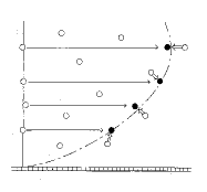
Figure 1: A flow through a capillary.

The change of the starting point from Eq.(2) to Eq.(4) opens a new possibility. Using the Kramers-Kronig relation, we will relate the frictionless capillary flow with the nonclassical flow in a rotating bucket. This method originated in studies of electron superconductivity fer . Between the above two forms of superfluidity in liquid helium 4, we find a parallel relationship to that between the electrical conduction and the Meissner effect in superconductivity. This analogy permits to express $1/\eta$ in terms of the susceptibility of the system, and enables to include the effect of Bose statistics into the perturbation expansion.

As an application of this method, we examine the gradual fall of $\eta(T)$ with decreasing temperature of liquid helium 4 from $3.7K$ to $T_{\lambda}$ in $1$ atm. It is often said that this $\eta(T)$ resembles $\eta(T)$ of a gas than a liquid in its magnitude and in its temperature dependence. But this expression is somewhat misleading, because the picture of a gas has no ground in this regime. Rather, we must consider this gradual fall of $\eta(T)$ as a property of the liquid under the strong influence of Bose statistics.

This paper is organized as follows. Section 2.A considers the shear viscosity of liquid helium 4 using Kramers-Kronig relation, and gives a formula for the kinematic shear viscosity $\nu(T)$. Section.2.B discusses the physical reason for the suppression of the shear viscosity by Bose statistics. Sec.3 examines the shear viscosity of liquid helium 4 above $T_{\lambda}$, and Sec.4 makes a comparison to experiments. Section.5 discusses some related problems.

II Shear viscosity of a Bose liquid

II.1 Formalism

For liquid helium 4, we use the following hamiltonian with the repulsive interaction $U$

$$H=\sum_{p}\epsilon(p)\Phi_{p}^{\dagger}\Phi_{p}+U\sum_{p,p^{\prime}}\sum_{q}\Phi_{p-q}^{\dagger}\Phi_{p^{\prime}+q}^{\dagger}\Phi_{p^{\prime}}\Phi_{p},\qquad(U>0),$$ (5)

where $\Phi_{p}$ denotes an annihilation operator of a spinless boson.

Let us generalize Eq.(4) to the case of the oscillatory pressure as follows

$$\mbox{\boldmath$j$}(\omega)=-\sigma(\omega)a^{2}\frac{\Delta\mbox{\boldmath$P$}(\omega)}{L}.$$ (6)

The conductivity spectrum $\sigma(\omega)$ in Eq.(6) must satisfy the following sum rule sum

$$\frac{1}{\pi}\int_{0}^{\infty}\sigma(\omega)d\omega=f(a),$$ (7)

where $f(a)$ is a function determined by fluid dynamics. Equation (7) is a form of the oscillator-strength sum rule in terms of fluid conductivity through a capillary. The Stokes equation gives an expression of $\sigma(\omega)$ and $f(a)$ (see Appendix.A).

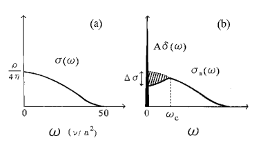
Figure 2: The change of the conductivity spectrum $\sigma(\omega)$ from (a) at $T>T_{\lambda}$ to (b) at $T<T_{\lambda}$. At $T>T_{\lambda}$, $\sigma(\omega)$ is given by the real part of Eq.(A5). At $T<T_{\lambda}$, the sharp peak with a half width $\omega_{s}$ and an area $A$ appears around $\omega=0$. $\omega_{c}$ is a frequency at the broad peak of $\sigma_{n}(\omega)$.

At $T<T_{\lambda}$, a frictionless flow appears in Eq.(6). Characteristic to the frictionless flow is the fact that in addition to the normal fluid part $\sigma_{n}(\omega)$, the conductivity spectrum $\sigma(\omega)$ has a sharp peak at $\omega=0$ (with a very small but finite half width $\omega_{s}$). Hence, one obtains

$$\mbox{\boldmath$j$}(\omega)=-\left[\sigma_{n}(\omega)+A\delta(\omega)\right]a^{2}\frac{\Delta\mbox{\boldmath$P$}(\omega)}{L},$$ (8)

where $\delta(\omega)$ is a simplified expression of the sharp peak at $\omega=0$, and $A$ is an area of this peak fer . Figure 2 schematically illustrates such a change of $\sigma(\omega)$ when the system passes $T_{\lambda}$. When $\sigma(\omega)$ has a form of $\sigma_{n}(\omega)+A\delta(\omega)$, $\eta$ in Eq.(4) is given by

$$\eta(T)=\frac{1}{4}\frac{\rho}{\sigma_{n}(0)+\displaystyle{\left(\frac{A}{\omega_{s}}\right)}}.$$ (9)

In view of Eq.(9), the sharpness of the peak at $\omega=0$ ($\omega_{s}\simeq 0$) leads to the disappearance of the shear viscosity ($\eta(T)\simeq 0$) at $T<T_{\lambda}$.

Let us generalize Eq.(6) so that it includes not only a mass flow responding in phase with $\Delta\mbox{\boldmath$P$}(\omega)$ but also a mass flow responding out of phase. $\sigma(\omega)$ in Eq.(6) is generalized to a complex number $\sigma_{1}+i\sigma_{2}$ as follows

$$\mbox{\boldmath$j$}(\omega)=-\left[\sigma_{1}(\omega)+i\sigma_{2}(\omega)\right]a^{2}\frac{\Delta\mbox{\boldmath$P$}(\omega)}{L},$$ (10)

where $\sigma(\omega)$ in Eq.(6) is replaced by $\sigma_{1}(\omega)$. Instead of $\Delta\mbox{\boldmath$P$}(t)$, we will use a fictitious velocity $\mbox{\boldmath$v$}(t)$ in Eq.(10). Applying the pressure gradient to a liquid is equivalent to assuming, as an external field, a velocity $\mbox{\boldmath$v$}(t)$ satisfying the equation of motion vec

$$\rho\frac{d\mbox{\boldmath$v$}(t)}{dt}=-\frac{\Delta\mbox{\boldmath$P$}(t)}{L}.$$ (11)

When replacing $\Delta\mbox{\boldmath$P$}(\omega)/L$ with $-i\rho\omega\mbox{\boldmath$v$}(\omega)$ in Eq.(10), the real and imaginary part of $\sigma(\omega)$ are interchanged,

$$\mbox{\boldmath$j$}(\omega)=\rho\left[-\omega\sigma_{2}(\omega)+i\omega\sigma_{1}(\omega)\right]a^{2}\mbox{\boldmath$v$}(\omega).$$ (12)

Equation (12) is a linear-response formula, in which $\mbox{\boldmath$j$}(\omega)$ and $\mbox{\boldmath$v$}(\omega)$ forms a perturbation energy such as $\mbox{\boldmath$j$}(\omega)\cdot\mbox{\boldmath$v$}(\omega)$ vel . The susceptibility $\chi(\omega)$ consists of a real part $-\omega\sigma_{2}(\omega)$ for the non-dissipative flow and an imaginary part $i\omega\sigma_{1}(\omega)$ for the dissipative one.

Causality requires that one observes a mass flow only after the pressure is applied. We obtain the following Kramers-Kronig relation for $-\omega\sigma_{2}(\omega)$ and $\omega\sigma_{1}(\omega)$ in Eq.(12)

$$\sigma_{1}(\omega^{\prime})=\frac{2}{\pi}\int_{0}^{\infty}d\omega\frac{\omega\sigma_{2}(\omega)}{\omega^{2}-\omega^{\prime 2}},$$ (13)

$$\omega^{\prime}\sigma_{2}(\omega^{\prime})=-\frac{2}{\pi}\int_{0}^{\infty}d\omega\frac{\omega^{2}\sigma_{1}(\omega)}{\omega^{2}-\omega^{\prime 2}}.$$ (14)

If one determines $\sigma_{2}(\omega)$ in the non-dissipative flow, one obtains $\sigma_{1}(\omega)$ using Eq.(13).

As a non-dissipative flow, we consider a flow in a rotating bucket. In fluid dynamics, the viscous dissipation in an incompressible fluid is estimated by the dissipation function

$$\Phi(\mbox{\boldmath$r$})=2\eta\left(e_{ij}-\frac{1}{3}e_{kk}\delta_{ij}\right)^{2},$$ (15)

($e_{ij}=(\partial v_{i}/\partial x_{j}+\partial v_{j}/\partial x_{i})/2$ is the shear velocity). Different flow patterns have different degrees of dissipation: For the Poiseuille flow Eq.(3), the dissipation function Eq.(15) is not zero at every $r$ except for $r=0$. Fluid particles in a capillary flow experience thermal dissipation not only at the boundary, but also inside of the flow. On the other hand, in a rotating bucket, a liquid makes the rigid-body rotation owing to its viscosity. Except at the boundary to the wall, there is no frictional force within a liquid, and the flow is therefore a non-dissipative one. (The velocity is a product of the radius and the rotational velocity $\Omega$ such as $\mbox{\boldmath$v$}_{d}(\mbox{\boldmath$r$})\equiv\mbox{\boldmath$\Omega$}\times\mbox{\boldmath$r$}$, for which Eq.(15) is zero at every $r$.)

The flow in a rotating bucket is formulated using the generalized susceptibility of the system $\chi(\mbox{\boldmath$r$},\omega)$ noz . When we assume $\mbox{\boldmath$v$}_{d}(\mbox{\boldmath$r$},t)=\mbox{\boldmath$\Omega$}\times\mbox{\boldmath$r$}e^{i\omega t}$ as a $\mbox{\boldmath$v$}(\omega)$ in Eq.(12), $\mbox{\boldmath$j$}(\mbox{\boldmath$r$},\omega)$ and $\mbox{\boldmath$v$}_{d}(\mbox{\boldmath$r$},\omega)$ form the perturbation energy like $\int dx\mbox{\boldmath$v$}_{d}\cdot\mbox{\boldmath$j$}$. Since the flow in a rotating bucket is a non-dissipative system, $\mbox{\boldmath$j$}(\mbox{\boldmath$r$},\omega)$ is a dynamical response of a liquid to the mechanical external field $\mbox{\boldmath$v$}_{d}(\mbox{\boldmath$r$},\omega)$, such as $\mbox{\boldmath$j$}(\mbox{\boldmath$r$},\omega)=\chi(\mbox{\boldmath$r$},\omega)\mbox{\boldmath$v$}_{d}(\mbox{\boldmath$r$},\omega)$. The influence of the wall motion propagates from the wall to the center along the radial direction, which is perpendicular to the particle motion driven by rotation. Hence, the flow in a rotating bucket is a transverse response described by the transverse susceptibility $\chi^{T}(q,\omega)$. In the right-hand side of Eq.(12), the real part $-\rho\omega\sigma_{2}(\omega)a^{2}$ is expressed as

$$-\rho a^{2}\omega\sigma_{2}(\omega)=\lim_{q\to 0}\chi^{T}(q,\omega).$$ (16)

Using Eq.(16) in the right-hand side of Eq.(13), we obtain $\sigma_{1}(\omega)$ for the capillary flow

$$\rho a^{2}\sigma_{1}(\omega^{\prime})=-\frac{2}{\pi}\int_{0}^{\infty}d\omega\frac{\lim_{q\to 0}\chi^{T}(q,\omega)}{\omega^{2}-\omega^{\prime 2}}.$$ (17)

Equation(17) has the following meaning. Quantum mechanics states that, in the decay from an excited state with an energy level $E$ to a ground state with $E_{0}$, the higher excitation energy $E$ causes the shorter relaxation time $\tau$. The time-dependent perturbation theory says

$$\frac{\hbar}{\tau}\simeq|E-E_{0}|.$$ (18)

In Eq.(17), the left-hand side includes the relaxation time $\tau$ as $\sigma_{1}=\rho/(4\eta)=\rho/(4G\tau)$ (see Appendix.B), whereas the right-hand side includes the excitation spectrum in $\chi^{T}(q,\omega)$. In this sense, Eq.(17) is a many-body theoretical expression of Eq.(18).

In the normal fluid phase, $\chi^{L}(q,\omega)=\chi^{T}(q,\omega)$ is satisfied at small $q$ and $\omega$, and one can replace $\chi^{T}(q,\omega)$ in Eq.(17) by $\chi^{L}(q,\omega)$ for a small $q$ and $\omega$ def . Hence, the conductivity $\sigma_{1n}(\omega)$ of the capillary flow in the normal fluid phase is given by

$$\rho a^{2}\sigma_{1n}(\omega^{\prime})=-\frac{2}{\pi}\int_{0}^{\infty}d\omega\frac{\lim_{q\to 0}\chi^{L}(q,\omega)}{\omega^{2}-\omega^{\prime 2}}.$$ (19)

In the superfluid phase, under the strong influence of Bose statistics, the condition of $\chi^{L}(q,\omega)=\chi^{T}(q,\omega)$ at $q\rightarrow 0$ is violated (see Sec.2.B). Consequently, one cannot replace $\chi^{T}(q,\omega)$ by $\chi^{L}(q,\omega)$ in Eq.(17). In addition to $\sigma_{1n}(\omega)$, one must separately consider the contribution of $\chi^{T}(q,\omega)-\chi^{L}(q,\omega)$. Hence, one obtains

$$\sigma_{1}(\omega^{\prime})=\sigma_{1n}(\omega^{\prime})+\frac{2}{\rho\pi a^{2}}\int_{0}^{\infty}d\omega\frac{\lim_{q\to 0}[\chi^{L}(q,\omega)-\chi^{T}(q,\omega)]}{\omega^{2}-\omega^{\prime 2}},$$ (20)

in which $\lim_{q\to 0}[\chi^{L}(q,\omega)-\chi^{T}(q,\omega)]$ corresponds to a superfluid component. In general, superfluidity is not rigid against external perturbations oscillating at not low frequencies: Above a certain $\omega_{0}$, $\lim_{q\to 0}[\chi^{L}(q,\omega)-\chi^{T}(q,\omega)]$ becomes zero. One can see $\sigma_{1}(\omega)$ of such a system using a simple example. We assume a constant $\lim_{q\to 0}[\chi^{L}(q,0)-\chi^{T}(q,0)]$ for $0\leq\omega\leq\omega_{0}$, and $0$ for $\omega_{0}<\omega$. In this case, we obtain

$$\sigma_{1}(\omega)=\sigma_{1n}(\omega)+\frac{2}{\rho\pi a^{2}}\lim_{q\to 0}[\chi^{L}(q,0)-\chi^{T}(q,0)]D_{\omega_{0}}(\omega).$$ (21)

where

$$D_{\omega_{0}}(\omega)=\frac{1}{2\omega}\ln|\frac{\omega_{0}^{2}}{\omega^{2}}-1|.$$ (22)

Figure.3 shows $D_{\omega_{0}}(\omega)$ for $\omega_{0}=1$. For every $\omega_{0}$, $D_{\omega_{0}}(\omega)$ resembles the $\delta(\omega)$-function. This simple example suggests that, for all probable forms of $\lim_{q\to 0}[\chi^{L}(q,\omega)-\chi^{T}(q,\omega)]$, the sharp peak around $\omega=0$ is a general feature of $\sigma_{1}(\omega)$. On comparing Eqs.(21) and (22) with Eq.(8), we obtain an expected form of $\sigma(\omega)$ for the superfluid flow, and $A=2\lim_{q\to 0}[\chi^{L}(q,0)-\chi^{T}(q,0)]/(\rho\pi a^{2})$. The half width $\omega_{s}$ of the peak in $\sigma_{1}(\omega)$ is determined by $\omega_{0}$ in $\chi^{L}-\chi^{T}$, and it gives us a measure for the rigidity of superfluidity.

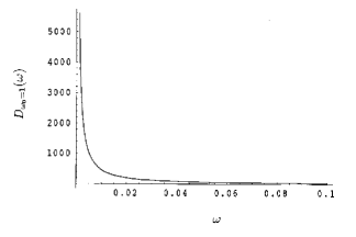
Figure 3: $D_{\omega_{0}}(\omega)$ for $\omega_{0}=1$.

When the system passes $T_{\lambda}$, $\sigma(\omega)$ changes from Fig.2(a) to 2(b) under the sum rule Eq.(7). The area $A$ of the sharp peak is equal to that of the shaded region in Fig.2(b). At $\omega=0$, the conductivity is enhanced by the sharp peak as $A/\omega_{s}$, but the original $\sigma(0)$ becomes $\sigma(0)-\Delta\sigma$ by the sum rule. We approximate the shaded region in Fig.2(b) by a triangle. (A broad peak of $\sigma_{n}(\omega)$ is located at $\omega_{c}$). We take into account the sum rule as $-\Delta\sigma\omega_{c}/2+A=0$, hence $\Delta\sigma=2A/\omega_{c}$. After all, the conductivity at $\omega=0$ becomes $[\sigma(0)-2A/\omega_{c}]+A/\omega_{s}$ at $T<T_{\lambda}$. Using this form of $\sigma(0)$ and the expression of $A$, one obtains $\eta=\rho/(4\sigma(0))$ as

$$\eta(T)=\left(\frac{\rho}{4}\right)\frac{1}{\sigma_{1n}(0)+\displaystyle{\frac{2}{\rho\pi a^{2}}\left(\frac{1}{\omega_{s}}-\frac{2}{\omega_{c}}\right)\lim_{q\to 0}[\chi^{L}(q,0)-\chi^{T}(q,0)]}}.$$ (23)

Here, we define the mechanical superfluid density $\hat{\rho_{s}}(T)\equiv\lim_{q\to 0}[\chi^{L}(q,0)-\chi^{T}(q,0)]$, which does not always agree with the conventional thermodynamical superfluid density $\rho_{s}(T)$. (By “thermodynamical”, we imply the quantity that remains finite in the $V\rightarrow\infty$ limit.) Using $\omega_{s}\ll\omega_{c}$ in Eq.(23), we obtain the following formula of the kinematic shear viscosity $\nu(T)=\eta(T)/\rho(T)$

$$\nu(T)=\frac{\nu_{n}}{1+\displaystyle{\frac{8}{\pi a^{2}\omega_{s}}\frac{\hat{\rho_{s}}(T)}{\rho}}\nu_{n}},$$ (24)

where $\nu_{n}$ is the kinematic shear viscosity in the normal fluid phase, and it satisfies $\sigma_{1n}(0)=\rho/(4\eta_{n})=1/(4\nu_{n})$ in Eq.(23). (The total density $\rho$ in Eq.(23) slightly and monotonically increases with decreasing temperature from $4.2K$ to $T_{\lambda}$ ker . Comparing Eq.(24) with (23), we see that $\nu(T)=\eta(T)/\rho(T)$ is a more appropriate quantity than $\eta(T)$ for describing the change of the system around $T_{\lambda}$.)

One notes the following features in the formula (24).

(1) $\nu(T)$ of a superfluid is expressed as an infinite power series of $\nu_{n}$, and the influence of Bose statistics appears in its coefficients. This result does not depend on a particular model of a liquid, but on the general argument. (The microscopic derivation of $\nu_{n}$ depends on the model, which is a subject of the liquid theory and beyond the scope of this paper.)

(2) Because of $\omega_{s}\simeq 0$, which characterizes the sharp peak in Fig.2(b), a small change of $\hat{\rho_{s}}(T)$ in the denominator of the right-hand side is strongly enhanced to an observable change of $\nu(T)$.

(3) The existence of $1/a^{2}$ in front of $\hat{\rho_{s}}(T)/\rho$ indicates that a frictionless superfluid flow appears only in a narrow capillary with a small radius $a$: A narrower capillary shows a clearer evidence of a frictionless flow.

II.2 Physical interpretation

There is a physical reason to expect that the shear viscosity of a Bose liquid falls off at low temperature. For the shear viscosity of a classical liquid, Maxwell obtained a simple formula $\eta=G\tau$ (Maxwell’s relation) using a physical argument max . ($G$ is the modulus of rigidity. $\tau$ is a relaxation time of the process in which the fluid motion relaxes the shear stress between adjacent layers in a flow. See Appendix.B). In the vicinity of $T_{\lambda}$, no apparent structural transformation is observed in liquid helium 4. Hence, $G$ may be a constant at the first approximation, and therefore the fall of the shear viscosity is attributed to a decrease of $\tau$. In view of Eq.(18), the decrease of $\tau$ suggests that the excitation energy $E$ increases owing to Bose statistics. The relationship between the excitation energy and Bose statistics dates back to Feynman’s argument on the scarcity of the low-energy excitation in liquid helium 4 fey1 , in which he explained how Bose statistics affects the many-body wave function in configuration space. To the shear viscosity, we will apply his explanation.

Consider a flow in Fig.1. White circles represent an initial distribution of fluid particles. The long thin arrows move white circles on a solid straight line to black circles on a one-point-dotted-line curve. (A viscous liquid shows such a spatial gradient of the velocity. The influence of adjacent layers in a flow propagates along a direction perpendicular to the particle motion. Hence, the excitation caused by the shear viscosity is a transverse excitation.) Let us assume that a liquid in Fig.1 is in the Bose-Einstein Condensation (BEC) phase, and the many-body wave function has permutation symmetry everywhere in a capillary. At first sight, these displacements by long arrows seem to be a large-scale configuration change, but they are reproduced by a set of slight displacements by short thick arrows from the initial particles. In contrast with the longitudinal displacement, the transverse displacement does not change the particle density in the large scale, and therefore, to any given particle after displacement, it is always possible to find a particle being close to that particle in the initial configuration log . In Bose statistics, owing to permutation symmetry, one cannot distinguish between two types of particles after displacement, one moved from the neighboring position by the short arrow, and the other moved from distant initial positions by the long arrow. Even if the displacement made by the long arrows is a large displacement in classical statistics, it is only a slight displacement by the short arrows in Bose statistics .

Let us imagine this situation in 3N-dimensional configuration space. The excited state made of slight displacements, which is a characteristic of Bose statistics, lies in a small distance from the ground state in configuration space. Since the wave function of the excited state is orthogonal to that of the ground state in the integral over configurations, the amplitude of the many-body wave function of the excited state must spatially oscillate around zero. Accordingly, it oscillates within a small distance in configuration space. The kinetic energy of the system is determined by the 3N-dimensional gradient of the many-body wave function in configuration space, and therefore this steep rise and fall of the amplitude raises the excitation energy of this wave function. The relaxation from such an excited state is a rapid process with a small $\tau$. This mechanism explains why Bose statistics leads to the small coefficient of shear viscosity $\eta=G\tau$.

When the system is at high temperature, the coherent wave function has a microscopic size. If a long arrow in Fig.1 takes a particle to a position beyond the coherent wave function including that particle, one cannot regard the particle after displacement as an equivalent of the initial one. The mechanism below $T_{\lambda}$ does not work for the large displacement extending over two different wave functions. Hence, the relaxation time $\tau$ changes to an ordinary long $\tau$, which is characteristic of a normal liquid ber .

III shear viscosity above $T_{\lambda}$

Figure 4 shows $\nu(T)$ of liquid helium 4 in the vicinity of $T_{\lambda}$ bar . One notes that $\nu(T)$ does not abruptly drops to zero at $T_{\lambda}$. Rather, after reaching a maximum value at 3.7K, it gradually decreases with decreasing temperature, and finally drops to zero at the $\lambda$-point. $\nu(T)$ of a classical liquid ($\nu_{n}$ in Eq.(24)) has the general property of increasing monotonically with decreasing temperature she . In Fig.4, $\nu$ above $3.7K$ seems to follow this property, whereas its gradual fall below $3.7K$ suggests $\hat{\rho_{s}}(T)\neq 0$ in Eq.(24) at $T_{\lambda}\leq T\leq 3.7K$ spe .

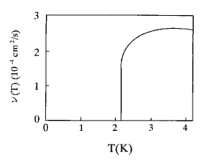
Figure 4: The temperature dependence of the kinematic shear viscosity $\nu(T)$ of liquid helium 4 obtained in Ref.bar .

In an ideal Bose gas, one knows $\hat{\rho_{s}}(T)=0$ at $T>T_{\lambda}$, hence obtains $\nu(T)=\nu_{n}$ at $T>T_{\lambda}$ in Eq.(24). This means that, without the interaction between particles, BEC is the necessary condition for the superfluid flow. To explain the gradual fall of $\nu(T)$ just above $T_{\lambda}$, we must obtain $\chi^{L}(q,\omega)-\chi^{T}(q,\omega)$ under the repulsive interaction $U$. The susceptibility is decomposed into the longitudinal and transverse part ($\mu,\nu=x,y,z$)

$$\chi_{\mu\nu}(q,\omega)=\frac{q_{\mu}q_{\nu}}{q^{2}}\chi^{L}(q,\omega)+\left(\delta_{\mu\nu}-\frac{q_{\mu}q_{\nu}}{q^{2}}\right)\chi^{T}(q,\omega).$$ (25)

For the later use, we define a term proportional to $q_{\mu}q_{\nu}$ in $\chi_{\mu\nu}$ by $\hat{\chi}_{\mu\nu}=(q_{\mu}q_{\nu}/q^{2})[\chi^{L}(q,\omega)-\chi^{T}(q,\omega)]$ for considering $\hat{\rho_{s}}(T)=\lim_{q\to 0}[q^{2}/(q_{\mu}q_{\nu})]\hat{\chi}_{\mu\nu}$. Under the repulsive interaction $\hat{H_{I}}(\tau)$, $\hat{\chi}_{\mu\nu}$ is derived from

$$<G|T_{\tau}J_{\mu}(x,\tau)J_{\nu}(0,0)|G>=\frac{\displaystyle{<0|T_{\tau}\hat{J}_{\mu}(x,\tau)\hat{J}_{\nu}(0,0)exp\left[-\int_{0}^{\beta}d\tau\hat{H}_{I}(\tau)\right]|0>}}{\displaystyle{<0|exp\left[-\int_{0}^{\beta}d\tau\hat{H}_{I}(\tau)\right]|0>}},$$ (26)

where $J_{\mu}(q,\tau)=\sum_{p,n}(p+q/2)_{\mu}\Phi_{p}^{\dagger}\Phi_{p+q}e^{-i\omega_{n}\tau}$, ($\beta=1/(k_{B}T),\tau=it$). Compared to an ordinary liquid, liquid helium 4 above $T_{\lambda}$ has a $10^{-3}$ times smaller coefficient of shear viscosity as shown in Fig.4. Although in the normal phase, it is already an anomalous liquid under the strong influence of Bose statistics. Hence, it seems natural to assume that, as $T\rightarrow T_{\lambda}$ in the normal phase, large but not yet macroscopic coherent wave functions gradually grow as a thermal equilibrium state, and suppress the shear viscosity lod .

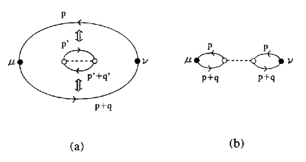
Figure 5: Exchange of particles in (a) between $J_{\mu}J_{\nu}$ (a large bubble) and a bubble excitation (an inner small one) yields (b).

Here, we summarize the result of Ref.koh , which formulates the interpretation in Sec.2B. Figure 5 illustrates the current-current response tensor $\hat{J}_{\mu}(x,\tau)\hat{J}_{\nu}(0,0)$ (a large bubble with $\mu$ and $\nu$) in the liquid: Owing to $exp(-\smallint\hat{H}_{I}(\tau)d\tau)$, scattering of particles frequently occurs as illustrated by an inner small bubble with a dotted line $U$. As the order of the perturbation increases, $\hat{J}_{\mu}(x,\tau)\hat{J}_{\nu}(0,0)$ in the vicinity of $T_{\lambda}$ gradually reveals a new effect due to Bose statistics: The large bubble $\hat{J}_{\mu}(x,\tau)\hat{J}_{\nu}(0,0)$ and the small bubble in Fig.5(a) form a coherent wave function as a whole com : When one of the two particles in the large bubble and in the small bubble have the same momentum ($p=p^{\prime}$), and when the other in both bubbles have another same momentum ($p+q=p^{\prime}+q^{\prime}$), Bose statistics forces us to include in the expansion a graph made by exchanging these particle. This exchange yields Fig.5(b), in which two bubbles with the same momenta are linked by the repulsive interaction. With decreasing temperature, the coherent wave function grows, and such an exchange of particles occurs many times. Furthermore, among possible physical processes, processes including $p=0$ particles get to play a more dominant role than others: In Fig.5, a bubble with $p=0$ corresponds to an excitation from the rest particle, and a bubble with $p=-q$ corresponds to a decay into the rest one. Taking only such processes and continuing these exchanges, one obtains $\hat{\chi}_{\mu\nu}(q,0)$ for $\hat{\rho_{s}}(T)$

$$\hat{\chi}_{\mu\nu}(q,0)=\frac{q_{\mu}q_{\nu}}{2}\frac{1}{V}\frac{F_{\beta}(q)}{1-UF_{\beta}(q)},$$ (27)

where

$$F_{\beta}(q)=\frac{(\exp(\beta[\Sigma-\mu])-1)^{-1}-(\exp(\beta[\epsilon(q)+\Sigma-\mu])-1)^{-1}}{\epsilon(q)}$$ (28)

is a positive and monotonically decreasing function of $q^{2}$, which approaches zero as $q^{2}\rightarrow\infty$. An expansion of $F_{\beta}(q)$ around $q^{2}=0$, $F_{\beta}(0)-bq^{2}+\cdots$ has a form such as

$$F_{\beta}(q)=\frac{\beta}{4\sinh^{2}\displaystyle{\left(\frac{|\beta[\mu(T)-\Sigma]}{2}\right)}}\left[1-\frac{\beta}{2}\frac{1}{\tanh\displaystyle{\left(\frac{|\beta[\mu(T)-\Sigma]|}{2}\right)}}\frac{q^{2}}{2m}+\cdots\right].$$ (29)

(a) With decreasing temperature, $\mu$ gradually approaches $\Sigma$. As $\mu-\Sigma\rightarrow 0$, $F_{\beta}(q)$ in Eq.(28) increases, and it creates a divergence in Eq.(27): This divergence first occurs at $q^{2}=0$, because $F_{\beta}(q)$ is a positive decreasing function of $q^{2}$. For a small $q$, $1-UF_{\beta}(q)$ in Eq.(27) is approximated as $[1-UF_{\beta}(0)]+Ubq^{2}$. As $\mu-\Sigma\rightarrow 0$, $UF_{\beta}(0)$ increases and finally reaches 1, that is,

$$U\beta=4\sinh^{2}\left(\frac{\beta[\mu(T)-\Sigma(U)]}{2}\right).$$ (30)

At this point, the denominator in Eq.(27) gets to begin with $q^{2}$, and $\hat{\chi}_{\mu\nu}(q,0)$ therefore has a form of $q_{\mu}q_{\nu}/q^{2}$ at $q\rightarrow 0$, the coefficient of which is $F_{\beta}(0)/(2VUb)$. By the definition of $\hat{\rho_{s}}(T)=\lim_{q\to 0}(q^{2}/q_{\mu}q_{\nu})\hat{\chi}_{\mu\nu}$, one obtains

$$\hat{\rho_{s}}(T)=\frac{1}{V}\frac{m}{\sinh|\beta[\mu(T)-\Sigma]|},$$ (31)

with the aid of Eqs.(29) and (30). Here, we call $T$ satisfying Eq.(30) the onset temperature $T_{on}$ of the nonclassical behavior.

(b) In the vicinity of $T_{\lambda}$, Eq.(30) is approximated as $U\beta=\beta^{2}[\mu(T)-\Sigma(U)]^{2}$ for a small $\mu-\Sigma$. This condition has two solutions $\mu(T)=\Sigma(U)\pm\sqrt{Uk_{B}T}$. The repulsive Bose system is generally assumed to undergo BEC as well as a free Bose gas. Hence, with decreasing temperature, $\mu(T)$ of repulsive Bose system should reach $\Sigma(U)$ at a finite temperature, during which course the system necessarily passes a state satisfying $\mu(T)=\Sigma(U)-\sqrt{Uk_{B}T}$. Consequently, $T_{on}$ is always above $T_{\lambda}$, and $\nu(T)$ deviates from $\nu_{n}$ just above $T_{\lambda}$ in Eq.(24).

(c) As $T$ approaches $T_{\lambda}$ from $T_{on}$, $\hat{\rho_{s}}(T)$ approaches $(m/V)[\exp(\beta[\mu(T)-\Sigma])-1]^{-1}$. This means that at $T=T_{\lambda}$, $\hat{\rho_{s}}(T_{\lambda})$ agrees with the conventional thermodynamical superfluid density $\rho_{s}(T_{\lambda})$, and it abruptly grows to a macroscopic number.

(d) At $T_{\lambda}<T<T_{on}$, Eq.(31) serves as an interpolation formula for $\hat{\rho_{s}}(T)$ pha .

IV Comparison to experiments

At an early stage in the study of superfluidity, $\eta(T)$ was measured by experiments using the capillary flow men tje zin . But early measurements have been superseded by that using more accurate techniques such as a vibrating wire goo wel bru . Above the $\lambda$ point, these different experimental methods give us quantitatively similar data on $\eta(T)$. Using these accumulated data, a precise curve of $\eta(T)$ and $\nu(T)$ above $T_{\lambda}$ was obtained by statistical analysis such as cubic spline fits bar . We will compare our formula with the results in Ref bar .

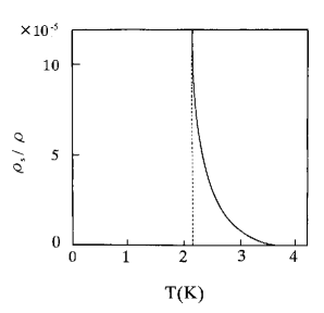
Figure 6: $\hat{\rho}_{s}(T)/\rho$ obtained by Eq.(32) using $\nu(T)$ in Fig.4.

(1) In Eq.(24), we assume $T_{on}=3.7K$ and $\nu_{n}=\nu(T_{on})$. We obtain $\hat{\rho}_{s}(T)/\rho$ by

$$\frac{8}{\pi a^{2}\omega_{s}}\frac{\hat{\rho}_{s}(T)}{\rho}=\nu(T)^{-1}-\nu(T_{on})^{-1}.$$ (32)

In the rotation experiment by Hess and Fairbank hes , the moment of inertia $I_{z}$ just above $T_{\lambda}$ is slightly smaller than the normal phase value $I_{z}^{cl}$ (see Sec.5.A). Using these data, Ref.koh roughly estimates $\hat{\rho}_{s}(T)/\rho$ as $\hat{\rho_{s}}(T_{\lambda}+0.03K)/\rho\cong 8\times 10^{-5}$, and $\hat{\rho_{s}}(T_{\lambda}+0.28K)/\rho\cong 3\times 10^{-5}$. The previous experiments in Ref.men tje zin differ in the capillary radius $a$. If we use a typical value $a\simeq 5\times 10^{-3}cm$, with these $\hat{\rho}_{s}(T)/\rho$ in Ref koh and $\nu(T)$ in Fig.4, we obtain a rough estimate of $\omega_{s}$ as $\omega_{s}\simeq 4\times 10^{-3}rad/s$. Figure 6 shows the temperature dependence of $\hat{\rho}_{s}(T)/\rho$ derived by using $\nu(T)$ (Fig.4) in Eq.(32). (The absolute value is adjusted to $\hat{\rho}_{s}/\rho$ at $T_{\lambda}+0.03K$ and $T_{\lambda}+0.28K$ in Ref koh . Since the precision of these values derived from currently available data is limited, the absolute value of $\hat{\rho}_{s}(T)/\rho$ in Fig.6 has a statistical uncertainty.)

(2) In Sec.3, we obtained the interpolation formula for $\hat{\rho}_{s}(T)/\rho$, Eq.(31). Here, we assume $\mu-\Sigma$ changes with temperature according to the formula

$$\mu(T)-\Sigma(U)=-\left(\frac{g_{3/2}(1)}{2\sqrt{\pi}}\right)^{2}k_{B}T_{\lambda}\left[\left(\frac{T}{T_{\lambda}}\right)^{3/2}-1\right]^{2},$$ (33)

($g_{a}(x)=\sum_{n}x^{n}/n^{a}$), where the particle interaction $U$ and the particle density $\rho$ of liquid helium 4 are renormalized to $T_{\lambda}=2.17K$. The temperature dependence of $\hat{\rho}_{s}(T)/\rho$ derived from Eqs.(31) and (33) bears a qualitative resemblance to $\hat{\rho}_{s}(T)/\rho$ in Fig.6. But, although remaining very small at $T_{\lambda}+0.2K<T<3.7K$, it abruptly grows at 2.3K, and reaches a macroscopic number at $T_{\lambda}$ (it resembles the shape of the letter $L$). Experimentally, however, as temperature decreases from 3.7K to $T_{\lambda}$, $\hat{\rho}_{s}(T)/\rho$ gradually grows as in Fig.6. This means that Eq.(31) is too simple to compare with the real system. With decreasing temperature, in addition to the particle with $p=0$, other particles having small but finite momenta get to contribute to the $1/q^{2}$ divergence of $\hat{\chi}_{\mu\nu}(q,0)$ as well. (In addition to Eq.(28), a new $F_{\beta}(q)$ including $p\neq 0$ also satisfies $1-UF_{\beta}(0)=0$ in Eq.(27).) The participation of $p\neq 0$ particles into $\hat{\rho_{s}}(T)$ is a physically natural phenomenon. For the repulsive Bose system, particles are likely to spread uniformly in coordinate space due to the repulsive force. This feature makes the particles with $p\neq 0$ behave similarly with other particles, especially with the particle having zero momentum. If they move at different velocities along the flow direction, the particle density becomes locally high, thus raising the interaction energy. This is a reason why many particles with $p\neq 0$ participate in a superfluid even above $T_{\lambda}$ den .

(3) For the rigidity of superfluidity, we used two types of phenomenological parameters in Sec.2. Among them, $\omega_{s}$ of the sharp peak in $\sigma_{1}(\omega)$ is useful for comparing the theory with experiments. The quantity which has a physically clear meaning, however, is $\omega_{0}$ in $\lim_{q\to 0}[\chi^{L}(q,\omega)-\chi^{T}(q,\omega)]$. As an example, we used a step function of $\omega$ with a width $\omega_{0}$. Its Hilbert transform $\sigma_{1}(\omega)$ in Eq.(22) shows a $\delta$-function-like peak with a width $\omega_{s}$ such as $\omega_{s}=10^{-3}\omega_{0}\sim 10^{-2}\omega_{0}$ in Fig.3. Since $\omega_{s}\cong 10^{-3}rad/s$, the critical frequency $\omega_{0}$ above which the condition of superfluidity $\lim_{q\to 0}\chi^{L}(q,\omega)\neq\lim_{q\to 0}\chi^{T}(q,\omega)$ is violated is $10^{-1}rad/s\sim 1rad/s$.

(4) Equations (30) and (33) with $T_{on}=3.7K$ gives us a rough estimate of $U$ as $U\sim 3.4\times 10^{-16}erg$, which is somewhat larger than the value obtained from the sound velocity using the Bogoliubov formula.

V Discussion

V.1 Superfluidity in the dissipative and the non-dissipative systems

On the onset mechanism of superfluidity, one can see physical differences between dissipative and non-dissipative flows. As an example of non-dissipative flows, we considered the flow in a rotating bucket in Sec.2, in which a quantity directly indicating the onset of superfluidity is the moment of inertia

$$I_{z}=I_{z}^{cl}\left(1-\frac{\hat{\rho_{s}}(T)}{\rho}\right),$$ (34)

where $I_{z}^{cl}$ is its classical value. Equation (34) and (24) have the following differences.

(a) In Eq.(34), $\hat{\rho_{s}}(T)$ appears as a correction to the coefficient of the linear term $I_{z}^{cl}$, whereas Eq.(24) has a form of infinite power series of $\nu_{n}$ and $\hat{\rho_{s}}(T)$. With decreasing temperature, the higher-order terms become dominant in Eq.(24).

(b) In Eq.(34), the change of $\chi^{L}-\chi^{T}$ affects $I_{z}$ without being enhanced, and therefore the small $\hat{\rho_{s}}(T)$ only slightly affects $I_{z}$ above $T_{\lambda}$ koh . In Eq.(24), the change of $\chi^{L}-\chi^{T}$ does not directly affect $\nu$, but through the dispersion integral as in Eq.(20). By this mechanism, a small change of the system leading to superfluidity is enhanced to an easily observable scale, which amplification mechanism does not appear in superfluidity in the non-dissipative systems.

(c) Equation (34) includes no phenomenological parameter, whereas Eq.(24) includes the parameter $\omega_{s}$ representing the measure of the rigidity of superfluidity. This feature is characteristic of superfluidity in the dissipative systems. The stability of a superfluid has been studied in the context of the critical velocity of the persistent current rep . To obtain $\omega_{s}$ or $\omega_{0}$, similar considerations are needed for the stability of a superfluid against oscillating perturbations such as the oscillating velocity $v(r)e^{i\omega t}$. This is a future problem.

Anomalously high thermal conductivity of liquid helium 4 at $T<T_{\lambda}$ is another example of superfluidity in the dissipative system. Heat flow $q$ is expressed as $q=-\kappa\nabla T$, where $\kappa$ is the coefficient of thermal conductivity. In the critical region above $T_{\lambda}$ ($T/T_{\lambda}-1<10^{-3}$), the rapid rise of $\kappa$ is observed. At $T=T_{\lambda}$, $\kappa$ jumps to an at least $10^{7}$ times higher value than $\kappa$ just above $T_{\lambda}$. In $T_{\lambda}<T<3.7K$, however, $\kappa$ does not show a symptom of its rise, in contrast with $\eta$ which shows a symptom of its fall in the same region kel . In the case of the capillary flow, we can assume the flow in a rotating bucket as a non-dissipative counterpart, whereas in the case of heat conduction, we do not know such a counterpart. Theoretically, the coefficient of thermal conductivity is expressed by a correlation function which has a formally similar form to that of the shear viscosity. But heat conduction is a transport phenomenon of energy. The scalar field (temperature field) has only a small variety of spatial distribution compared to the vector field (velocity field), and therefore heat conduction is always a dissipative phenomenon. Hence, we can not apply the formalism in this paper to the onset mechanism of the anomalous thermal conductivity. This formal difference between the shear viscosity and the thermal conductivity is consistent with the experimental difference between them at $T_{\lambda}<T<3.7K$.

V.2 Comparison to Fermi liquids

In liquid helium 3, the fall of the shear viscosity at $T_{c}$ is known as a parallel phenomenon to that of liquid helium 4. The formalism in Sec.2 is applicable to the shear viscosity of liquid helium 3 as well. For the behavior above $T_{c}$, however, there is a striking difference between liquid helium 3 and 4. The phenomenon occurring in fermions in the vicinity of $T_{c}$ is not a gradual growth of the coherent wave function, but a formation of the Cooper pairs from two fermions. (This difference evidently appears in the temperature dependence of the specific heat: $C(T)$ of liquid helium 3 above $T_{c}$ does not show a symptom of its rise.) Once the Cooper pairs are formed, they are composite bosons situated at low temperature and high density, and immediately jumps to the ESP or BW state. Hence, the shear viscosity of liquid helium 3 shows an abrupt drop at $T_{c}$ without a gradual fall above $T_{c}$.

In electron superconductivity, the fluctuation-enhanced conductivity $\sigma^{\prime}$ is observed above $T_{c}$ (see the text by M.Tinkham in fer ). In bulk superconductors, however, the ratio of $\sigma^{\prime}$ to the normal conductivity $\sigma_{n}$ is about $10^{-5}$ at the critical region, and zero outside of this region. Practically, it is unlikely that thermal fluctuations create a large change of $\sigma$ at temperatures outside of the critical region.

V.3 Velocimetry technique

Since the discovery of superfluidity in liquid helium 4, a lot of measurements have been done, but there is so little direct experimental information about the flow patterns. Among various visualization techniques used in ordinary liquids, particle image velocimetry (PIV), which records the motion of micrometre-scale solid particles suspended in the fluid as tracer particles, recently becomes available in superfluid helium 4. Until now, this technique has been mainly used for the study of turbulent flows don van , but it has the potential to give us more information. The quantity which directly indicates the onset of superfluidity in dissipative system is the change of the conductivity spectrum $\sigma(\omega)$. In view of the gradual decrease of $\eta$ above $T_{\lambda}$, the sharp peak at $\omega=0$ and the corresponding change from $\sigma(\omega)$ to $\sigma_{n}(\omega)$ in Fig.2 must already appear at $T>T_{\lambda}$. To confirm this prediction, under the slowly oscillating pressure, time-resolved measurement of the oscillating flow velocity $\mbox{\boldmath$v$}(\mbox{\boldmath$r$},t)$ is necessary. Such an experiment must be performed in a thin capillary with an inner radius of $10^{-2}\sim 10^{-1}$ mm. If the PIV experiment is performed under such conditions and the data of $\mbox{\boldmath$v$}(r=0,t)$ is Fourier-transformed, the change of $\sigma(\omega)$ in Fig.2 will be observed. Since quantized vortices are absent in the capillary flow, tracer particles interact only with the normal fluid part and trace its velocity poo . Hence, in Fig.2(b) only the change from $\sigma(\omega)$ to $\sigma_{n}(\omega)$ will be observed. The quantity $A$ in Eq.(8) is equal to the area of the shaded region $\sigma(\omega)-\sigma_{n}(\omega)$ in Fig.2(b). Using thus obtained $A$, one can determine $\omega_{s}$ by comparing the experimental data of $\eta(T)$ with Eq.(9). Furthermore, using $\pi a^{2}A=2\hat{\rho}_{s}(T)/\rho$, one will obtain a new estimate of $\hat{\rho}_{s}(T)/\rho$ at $T>T_{\lambda}$. Such an experiment may be a difficult one, but it will provide us valuable information.

Appendix A Conductivity spectrum $\sigma(\omega)$

The Stokes equation under the oscillatory pressure gradient $\Delta Pe^{i\omega t}/L$ is written in the cylindrical polar coordinate as follows

$$\frac{\partial v}{\partial t}=\nu\left(\frac{\partial}{\partial r^{2}}+\frac{\partial}{r\partial r}\right)v+\frac{\Delta Pe^{i\omega t}}{\rho L}.$$ (35)

The velocity has the following form

$$v(r,t)=\frac{\Delta Pe^{i\omega t}}{i\omega\rho L}+\Delta v(r,t),$$ (36)

with the boundary condition of $v(a,t)=0$. $\Delta v(r,t)$ satisfies

$$\frac{\partial\Delta v(r,t)}{\partial t}=\nu\left(\frac{\partial}{\partial r^{2}}+\frac{\partial}{r\partial r}\right)\Delta v(r,t),$$ (37)

and therefore $\Delta v(r,t)$ has a solution written by the Bessel function $J_{0}(i\lambda r)$ with $\lambda=(1+i)\sqrt{\omega/(2\nu)}$. Hence,

$$v(r,t)=\frac{\Delta Pe^{i\omega t}}{i\omega\rho L}\left(1-\frac{J_{0}(i\lambda r)}{J_{0}(i\lambda a)}\right).$$ (38)

At $r=0$, the conductivity spectrum $\sigma(\omega)$, which is given by $\rho v(0,t)=\sigma(\omega)a^{2}\Delta Pe^{i\omega t}/L$, has the following form

$$\sigma(\omega)=\frac{1}{i\omega a^{2}}\left(1-\frac{1}{J_{0}\left[ia(1+i)\displaystyle{\sqrt{\frac{\omega}{2\nu}}}\right]}\right).$$ (39)

The real part of Eq.(A5) gives a curve of $\sigma(\omega)$ in Fig.2(a) (Re $\sigma(0)=\rho/(4\eta)$), and determines $f(a)\propto a^{-2}$ in Eq.(7). ($\nu$ disappears in $\int\sigma(\omega)d\omega$.) Im $\sigma(\omega)$ gives an expression of $\sigma_{2}(\omega)$ in Eq.(10), but gives no concrete form of $\sigma_{2}(\omega)$ in Eq.(16), because it is derived from the phenomenological equation with dissipation like the Stokes equation.

Appendix B Maxwell’s relation

Consider shear transformation of a solid and of a liquid. In a solid, shear stress $F_{xy}$ is proportional to a shear angle $\phi$ as $F_{xy}=G\phi$, where $G$ is the modulus of rigidity. The value of $G$ is determined by dynamical processes in which vacancies in a solid move to neighboring positions over the energy barriers. As $\phi$ increases, $F_{xy}$ increases as follows,

$$\frac{dF_{xy}}{dt}=G\frac{d\phi}{dt}.$$ (40)

In a liquid, the motion of a fluid changes the relative positions of particles, reducing the shear stress $F_{xy}$ to a certain value. Presumably, the rate of such relaxations is proportional to the magnitude of $F_{xy}$, and one obtains

$$\frac{dF_{xy}}{dt}=G\frac{d\phi}{dt}-\frac{F_{xy}}{\tau},$$ (41)

where $\tau$ is a relaxation time. In the stationary flow after relaxation, $F_{xy}$ remains constant, and one obtains

$$G\frac{d\phi}{dt}=\frac{F_{xy}}{\tau}.$$ (42)

Figure.7 shows two particles 1 and 2, each of which starts at $(x,y)$ and $(x,y+\Delta y)$ simultaneously and moves along the $x$-direction. Assume that there is velocity gradient $v_{x}(y)$ along $y$ direction. After $\Delta t$ has passed, they (1’ and 2’) are at a distance of $\Delta v_{x}\Delta t$ along the $x$-direction. The shear angle increases from zero to $\Delta\phi$ as a result, which satisfies $\Delta v_{x}\Delta t=\Delta y\Delta\phi$ as depicted in Fig.7. Hence, we obtain

$$\frac{\partial v_{x}}{\partial y}=\frac{d\phi}{dt}.$$ (43)

Substituting Eq.(B4) into Eq.(B3), and comparing it with Eq.(1), one obtains $\eta=G\tau$ (Maxwell’s relation).

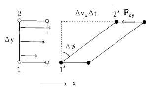
Figure 7: In a liquid flowing along the $x$-direction, owing to the velocity gradient along the $y$-direction, a small rectangular part of a liquid is deformed to a parallelogram.

References

- (1) L.D.Landau and I.M. Khalatonikov, Zh.Eksp.Teor.Fiz.19, 637, 709(1949), in Collected papers of L.D.Landau, (edited by D.ter.Haar, Pergamon, London, 1965).
- (2) L.P.Kadanoff and P.C.Martin, Ann.Phys. 24, 419(1963), P.C.Hoenberg and P.C.Martin, Ann.Phys. 34, 291(1965).
- (3) In the short time scale, the mechanism of the shear viscosity in a liquid is similar to that in a solid, and is therefore a highly inhomogeneous process at the molecular level: The modulus of rigidity is determined by the motion of vacancy as in a solid. (As a text, J.P.Hansen and I.R.McDonald, Theory of Simple Liquids, 3rd ed, (Academic Press, London, 2006)).
- (4) Using Eq.(2), of model is calculated beyond the one-loop level in the context of the relativistic heavy ion collision by S.Jeon, Phy.Rev.D.52, 3591(1995), E.Wang and U.Heinz, Phys.Lett.B. 52, 208(1999). These results describe the shear viscosity of a strongly interacting dense gas. For a liquid, however, the anisotropic particle interaction with the hard core must be introduced in calculations.
- (5) P.Kapitza, Nature.141, 74(1938), J.F.Allen and A.D.Misener, Nature.141, 75(1938)
- (6) As a response to , at another point is possible, but it results in the same form of .
- (7) To derive the decrease of from the increase of in Eq.(2), delicate cancellation of higher-order terms is needed in the perturbation expansion.
- (8) Just after the advent of BCS model, an attempt was made to relate the electrical conductivity (more precisely, the micro-wave absorption spectrum) with the penetration depth in the Meissner effect by R.A.Ferrell and R.E.Glover, Phy.Rev.109, 1398(1958), and by M.Tinkham and R.A.Ferrell, Phy.Rev.2, 331(1959). (As a text, M.Tinkham Introduction to superconductivity, 2nd ed, (McGraw-Hill, New York, 1996)). Whereas the electrical conduction is a dissipative phenomenon, the Meissner effect is a non-dissipative one, and is an analogue in superconductivity to the nonclassical flow in a rotating bucket noz .
- (9) R.Kubo, J.Phys.Soc.Japan.12, 570(1957).
- (10) In Ref fer , the definition of the vector potential plays the role of Eq.(11).
- (11) in the right-hand side of Eq.(12) is a fictitious velocity when the system would obey Eq.(11) of the non-interacting system, whereas included in of the left-hand side is a real velocity in the interacting system.
- (12) As a review, P.Nozieres, in Quantum Fluids (ed by D.E.Brewer), 1 (North Holland, Amsterdam, 1966), G.Baym, in Mathematical methods in Solid State and Superfluid Theory (ed by R.C.Clark and G.H.Derrick), 121 (Oliver and Boyd, Edingburgh, 1969)
- (13) We use in the transverse response such as conductivity despite of being a longitudinal susceptibility satisfying , which non obvious situation is explained by the replaceability of by in Eq.(19).
- (14) E.C.Kerr, J.Chem.Phys.26, 511(1957), and E.C.Kerr and R.D.Taylor, Ann.Phys. 26, 292(1964).
- (15) J.C.Maxwell, Phil.Trans.Roy.Soc.157, 49(1867) in The scientific papers of J.C.Maxwell, (edited by W.D.Niven, Dover, New York, 2003) Vol.2, 26.
- (16) R.P.Feynman, in Progress in Low Temp Phys. 1, (ed C.J.Gorter), 17 (North-Holland, Amsterdam, 1955).
- (17) For the longitudinal displacement, the large-scale inhomogeneity occurs in the particle density, and therefore it is not always possible to find such particles as in the transverse one.
- (18) The structural characteristic of liquids is irregular and only slightly different arrangements of molecules. The energies of these similar structures differ only slightly to each other. In the decays from one of these arrangements to others, the small leads to the long of a normal liquid.
- (19) C.F.Barenghi, P.J.Lucas, and R.J.Donnelly, J.Low.Temp.Phys.44, 491(1981)
- (20) In a classical liquid, is inversely proportional to the rate of processes in which vacancies in a liquid propagate from one point to another over the energy barriers. With decreasing temperature, this rate decreases. The liquid therefore gets to slowly respond to perturbations, and its increases.
- (21) This hypothesis is consistent with the specific heat of liquid helium 4, which shows a symptom of its rise at .
- (22) London stressed that the essence of superfluidity is not the absence of viscosity, but the occurrence of . (F.London Superfluid, John Wiely and Sons, New York, 1954 Vol.2, 141.) Although this remark is correct, it does not rule out the possibility that, behind the substantial decrease of above , is locally realized by the intermediate-sized coherent wave function. Since ordered motions of many particles are necessary for , we cannot attribute to the short-lived random fluctuations koh . (R.Bowers and K.Mendelssohn discussed a similar view on the nature of the decrease of above men .)
- (23) S.Koh, Phy.Rev.B.74, 054501(2006).
- (24) It is possible that more complex diagrams than a bubble exchange particles with the tensor . While it is difficult to estimate an infinite sum of these diagrams, it adds only a small correction.
- (25) R.A.Farrell, N.Menyhard, H.Schmidt, F.Schwabl and P.Szepfalusy, Ann.Phys. 47, 565(1968) considered the nonlocal superfluid density. This quantity, influenced by the phase fluctuation of the order parameter, only slightly deviates from the conventional within the range of . Our at is a different concept from this one.
- (26) R.Bowers and K.Mendelssohn, Proc.Roy.Soc.Lond.A.204, 366(1950)
- (27) H.Tjerkstra, Physica.19, 217(1953)
- (28) K.N.Zinoveva, Zh.Eksp.Teor.Fiz.34, 609(1958) [Sov.Phys-JETP.7, 421(1958)]
- (29) J.M.Goodwin, PhD Thesis, University of Washington (1968)
- (30) B.Welber, Phy.Rev.119, 1816(1960), B.Welber and D.C.Hammer, Phys.Lett.15, 233(1965), B.Welber and G.Allen, Phys.Lett.33A, 213(1970).
- (31) L.Bruschi, G.Mazzi, M.Santini and G.Torzo, J.Low.Temp.Phys.29, 63(1977)
- (32) G.B.Hess and W.M.Fairbank, Phy.Rev.19, 216(1967)
- (33) The total is a sum of each over different momenta. To avoid the rise of the repulsive interaction energy, fluid particles moving along the flow direction participate in . Hence, the density of states for this sum is not proportional to . Rather, the one-dimensional momenta along the flow direction leads to a constant density of states.
- (34) J.S.Langer and J.D.Reppy, in Progress in Low Temp Phys. 6, (ed C.J.Gorter), ch1 (North-Holland, Amsterdam, 1970).
- (35) L.J.Challis and J.Wilks, in Proceedings of the Symposium on Solid and Liquid (Ohio State University, Ohio, 1957). J.F.Kerrisk and W.E.Keller, Phy.Rev.177, 341(1969).
- (36) R.J.Donnelly,A.N.Karpetis, J.J.Niemela, K.R.Sreenivasan, W.F.Vinen and C.M.White, J.Low.Temp.Phys. 126, 327(2002),
- (37) T.Zhang, D.Celik and S.W.Van Sciver, J.Low.Temp.Phys. 134, 985(2004), T.Zhang and S.W.Van Sciver, J.Low.Temp.Phys. 138, 865(2005)
- (38) D.R.Poole, C.F.Barenghi, Y.A.Sergeev and W.F.Vinen, Phy.Rev.B.71, 064514(2005).