Data Assimilation for Wildland Fires
Ensemble Kalman filters in coupled atmosphere-surface models

December 2007, Revised January 2009

Wildfires represent a growing and costly hazard to society, particularly as homeowners build further into the wildland urban interface. Rather than a simple tactical response to put out a reported ignition, the sheer magnitude of areas engulfed in flames and intensity of the fires in fire prone areas such as southern California call for a strategic approach with forecasting tools to anticipate and mitigate fire behavior. Such tools do not currently exist.

A wildland fire is a complex multiscale process affected by nonlinear scale-dependent interactions with other Earth processes. Physical processes contributing to the fire occur over a wide range of scales. While the characteristic scales of weather processes range over 5 orders of magnitude from the hundred-km scale of large weather systems to the m-scale of small-scale effects and eddies, the chemical reactions associated with the thermal decomposition of fuel and combustion occur at scales of centimeters or less to produce flamelengths up to $60$-m tall. Firelines travel with average speeds on the order of a fraction of a m/s, while producing bursts of flame that travel at 50 m/s, and chemical reactions occur on the order of seconds or less. The wind and buoyancy produced by the fire are among the extremes of atmospheric phenomena. Weather is the major external factor that affects fire behavior, and two way interaction of fire and the atmosphere is essential – fires are known to dramatically influence the weather in their vicinity. The fire interacts with the atmosphere dynamics through fluxes of momentum, water vapor, and heat, and with the soil through moisture and heat retention.

Data do not come as exact coefficients and initial and boundary conditions for the model variables. Instead, various quantities only indirectly linked to the model variables are measured at discrete points spread over time and space, and the data are burdened with errors. Available data include fuel distribution maps, gridded atmospheric state from larger-scale weather models with assimilated weather data, point measurements from weather stations and fire sensors, two-dimensional airborne infrared imagery of the fire, and maps of fire extent produced by field personnel. The meteorological data are too sparse to resolve mesometeorological ($2$–$20$-km scale) features.

A computational model can capture only a select fraction of the significant mechanisms in the wildland fire process. Even if an accurate model existed, the data are not complete and accurate enough to make an accurate prediction possible. Also, one challenge of modeling is to estimate the accuracy of a forecast; a forecast has little value without additional information on what confidence level may be placed on it. Therefore, it is natural to consider statistics-based data assimilation methods. These methods include parameter and state estimation. Then the state of the model is the probability distribution of possible wildfire scenarios and the data are entered as data likelihood, which combines the information about the values of the measurements and the probability distribution of measurement errors. The data assimilation methods considered here proceed in analysis cycles. In each cycle, the model state is advanced in time, then new data are injected at the end of the cycle by combining the probability distribution of the state with the data likelihood.

However, the evolution of fire is highly nonlinear and the ignition is sharp or even discontinuous on the model scale. Statistical variability in additive corrections to the state may cause spurious ignitions, and additive corrections are not adequate to make changes to the location of the fire. Probability distribution of the fire state can be multimodal and centered around the burning and not burning states at any given point in space. The whole fire state may concentrate around more than one distinct scenario, such as whether or not the fire jumps a road.

Classical data assimilation methods, such as statistical interpolation, 3DVAR, and 4DVAR [1] represent probability distributions only by the mean and the covariance. But only the normal distribution is completely determined by the mean and the covariance, so the strong non-Gaussian character of fire makes the use of those methods questionable. The complexities of the model and sharp nonlinearities rule out adjoint methods, such as 3DVAR and 4DVAR, which are developed for atmospheric models, where the adjoint code can be produced by reversing the order of certain loops. Another option are ensemble methods. Although an ensemble can, in principle, represent a strongly non-Gaussian distribution, the EnKF [2] formulas are based on the assumption that the ensemble is a sample from a Gaussian distribution. Particle filters [3] also use an ensemble, and do not make the Gaussian assumption. However, particle filters are known to require a large ensemble size, which grows fast for high-dimensional problems. This requirement makes them generally unsuitable for problems with more than a handful of variables, in particular for fire models, which have millions of gridpoints, with several model variables associated with each gridpoint.

The goal of this article is to develop nontraditional ensemble Kalman filter methods for the forecast of the behavior of wildland fires. The ultimate goal is to estimate the state of the fire from available data and deliver a short-term prediction faster than real time taking into account the interactions between the fire and the atmosphere. Although fire is a complicated process, simple deterministic models that run fast can capture its essential behavior. Two such models are presented, a reaction-diffusion model based on simplified chemical kinetics [4], and a new level-set implementation of a semi-empirical fire propagation model [5] coupled with the Weather Research and Forecasting (WRF) atmospheric model [6]. The fire models are combined with two enhanced versions of the EnKF. The regularized EnKF [7] incorporates an assumption that the physical fields are (mostly) smooth, thus helping to prevent large variations in temperature and spurious ignition. The morphing EnKF [8] exploits methods of image processing to combine spatial and amplitude corrections to the state.

I How Should Wildland Fires Be Modeled?

In order to be faster than real time, fire models need to strike a balance between fidelity and fast execution. This article considers only two simplified 2D models for a fire in a layer just above the ground; see “Wildland Fire Modeling” for other approaches. Both models here are posed in the horizontal $\left(x_{1},x_{2}\right)$ plane, have a single vertical layer, and can be coupled with the atmosphere using the same variables. Their state variables and equations, however, are different.

The first model consists of the differential equations of chemical kinetics with two physical variables, the fuel temperature and the fuel mass. The speed of propagation of the fire is a property of the solution of the system of differential equations and thus it is determined by the coefficients of the equations only indirectly. In spite of its simplicity, this model captures naturally a number of fire phenomena, such as fire jumping a fuel break due to heat transfer across the break or fire being extinguished by increasing the heat outflow. On the other hand, the coefficients of the model are hard to calibrate to the observed fire behavior and the model requires a very fine grid and a very small time step to resolve the nonlinear effects in the leading edge of the fire, which is essential for correct fire propagation.

The second model is semi-empirical and it postulates the fire propagation speed normal to the fireline as a function of wind and terrain slope, and assumes an exponential decay of fuel from the time of ignition. Thus, the fire propagation speed can be input directly from known fire behavior for various fuels. The model can run on a relatively coarse grid, with the mesh step dictated only by the desired resolution of the shape of the fire region. The model has been validated on laboratory data and a number of forest fires. However, the model does not capture gradual changes in fire behavior, which would have to be implemented by ad-hoc modifications. The temperature or the fire intensity are not variables of this model and the heat produced is only a function of the time from ignition and of the fuel properties.

Although both models can be in principle coupled with an atmospheric model, we have implemented the coupling only for the semi-empirical model. These two models are representatives of the physics-based and semi-empirical approaches in wildfire modeling, respectively. Although a coupling of the two fire models could be considered, this was not done in the work presented, and either one or the other are used separately.

I-A Reaction-diffusion equations model

Consider a model consisting of a layer of fuel with concentration $F=F\left(x,t\right)$ ($kg/m^{2}$), $x=\left(x_{1},x_{2}\right)$ (m), and temperature $T=T\left(x,t\right)$ (K). The fuel is assumed to burn at the relative rate $r\left(T\right)$ $\left(\text{1/s}\right)$, dependent only on the temperature. The balance of heat in the fuel layer is described by the partial differential equation

$$c\frac{\partial T}{\partial t}=\nabla\cdot\left(k\nabla T\right)-(\overrightarrow{v}+\gamma\nabla z)\cdot\nabla T+\underbrace{AF\,r\left(T\right)-\overbrace{C\left(T-T_{a}\right)}^{H}}_{h\left(T\right)},$$ (1)

where $\nabla=\left(\frac{\partial}{\partial x_{1}},\frac{\partial}{\partial x_{2}}\right)$ is the gradient, $\cdot$ is the dot product, $c$, $k$, $A$, and $C$ are coefficients generally dependent on $x$ and $y$, $\overrightarrow{v}=\overrightarrow{v}\left(x,t\right)$ is the wind speed, and $\gamma\nabla z$ is the correction for the gradient of the terrain elevatin $z$ (since fire moves faster uphill). The term $c\frac{dT}{dt}$ is the heat flux (J/m²s) which is absorbed in the fuel and changes the fuel layer’s temperature. The diffusion term $\nabla\cdot\left(k\nabla T\right)$ models the heat transfer by short range radiation and air mixing, which causes the fire to spread between neighboring fuel particles (such as twigs and branches). The advection term $\overrightarrow{v}\cdot\nabla T$ is the heat flux due to wind. The external heat flux $h\left(T\right)$ consists of the heat flux $AFr\left(T\right)$, generated by burning the fuel, minus the heat flux

$$H=C\left(T-T_{a}\right),$$ (2)

escaping to the atmosphere at the ambient temperature $T_{a}$ according to the Newton’s law of cooling. The change in the fuel supply due to the burning is described by the fuel balance equation

$$\frac{dF}{dt}=-F\,r(T),$$ (3)

which is a collection of independent ordinary differential equations associated with the surface points $\left(x_{1},x_{2}\right)$. The reaction rate is taken to be

$$r\left(T\right)=De^{-B/(T-T_{a})},$$ (4)

where $B$ and $D$ are coefficients. The reaction rate (4) has the form of the Arrhenius reaction rate from chemical kinetics except for the offset $T_{a}$, which is to guarantee that the reaction rate is zero at the ambient temperature. Although the model (1)–(4) is simple, its solutions exhibit qualitative behaviors characteristic of combustion, known from chemical kinetics and the theory of reaction-diffusion equations [9, 10].

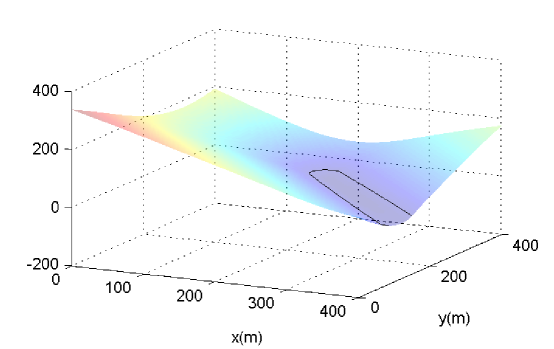
Neglecting for the moment the change in the fuel supply $F$, (1) has three equilibria, which are given by the zeros of the function $h\left(T\right)$ (Fig. 1). The smallest zero is the ambient temperature, where there is no reaction and no heat flux to the atmosphere. This smallest zero is a stable equilibrium because the derivative $h^{\prime}\left(T_{a}\right)<0$. The middle zero is the ignition temperature $T_{i}$, which is an unstable equilibrium, $h^{\prime}\left(T_{i}\right)>0$. At the ignition temperature, the heat generated by the reaction balances the heat escaping to the atmosphere, but a small increase of the temperature above $T_{i}$ creates a positive heat flux, which increases the temperature further, thus leading to the development of fire. The temperature climbs toward the largest zero of $h$, but then decreases as the fuel burns off following (3).

Solutions of the system (1)–(4) exhibit propagating combustion waves, at least for coefficients in certain ranges. At the leading edge of the combustion wave, the diffusion term spreads the heat into not-yet-ignited fuel and increases its temperature. Once the temperature is high enough for the heat generated by the reaction to overcome the heat loss, the temperature increases quickly and we say that the fuel ignites. The fuel then burns off and cools down, creating the trailing edge of the combustion wave. As a result, the combustion wave moves into yet-unburned fuel and leaves behind fuel burned down to a quantity no longer sufficient to sustain the reaction.

Unfortunately, taking coefficients from the physical and chemical properties of the fuel and expecting to obtain the correct combustion wave speed is hopeless. The reason is that coefficients are a homogenized form of unknown microscale data and many important physical processes are not modeled at all. For example, the model ignores the effect of the disappearance of fuel on the total heat capacity $c$ of the fuel layer, storage of the heat in the ground, the chemical kinetics of intermediate products of combustion, the fine scale fire dynamics on the surface and in the interior of the wood, and evaporation of moisture. Fortunately, suitable coefficients can be identified from observed macroscopic behavior of the fire. In [4], the coefficients are determined from temperature profile measured by a stationary sensor passed over by a moving combustion wave, and from the measured speed of the combustion wave (Fig. 2). Combustion wave speed is also called the fire spread rate.

The model (1)–(4) is discretized by standard finite difference techniques, with a sufficiently fine mesh to resolve the ignition region and upwinding of the advection term for stability. Ignition is achieved by an initial condition with a temperature well over the ignition temperature in a given ignition region, at least several meshcells large.

The computation visualized in Fig. 2 was done with mesh step size $2$ m on an interval $1000$ m long and time step $0.01$ s. A realistic fire model may require a domain size $10$ km by $10$ km, resulting in $50$ million variables. Mosaic character of fire makes the use of local mesh refinement difficult. Some fuels, such as grass, exhibit a reaction region only cm wide, thus requiring a mesh step of the order of $0.1$ m or less, which would result in models with more than $10^{11}$ variables.

I-B Fireline propagation model

The semi-empirical fire propagation model imposes the fire spread rate directly, replaces the leading edge of the combustion wave by instantaneous ignition, and replaces the fuel depletion rate by an imposed one.

Consider fire burning in the area $\Omega=\Omega\left(t\right)$ in the $\left(x_{1},x_{2}\right)$ plane, with the boundary $\Gamma=\Gamma\left(t\right)$, called the fireline, and with outside normal $\overrightarrow{n}=\overrightarrow{n}(x,t)$, $x\in$ $\Gamma\left(t\right)$. The time of ignition $t_{i}\left(x\right)$ at a point $x=\left(x_{1},x_{2}\right)\in$ $\Omega\left(t\right)$ is defined as the time when the point is at the fireline, $x\in\Gamma\left(t_{i}\left(x\right)\right)$.

The model postulates that the fireline evolves with a given spread rate $S=S\left(x,t\right)$ in the normal direction. The spread rate is a function of the is the components of the wind $\overrightarrow{v}$ and the terrain gradient $\nabla z$ in normal direction $\overrightarrow{n}$ to the fireline,

$$S=S\left(\overrightarrow{v}\cdot\overrightarrow{n},\nabla z\cdot\overrightarrow{n}\right)$$

as [5, 11]

$$S=\left\{\begin{tabular}[c]{ll}$0,$&if $\widetilde{S}<0,$\\ $S_{\max},$&if $\widetilde{S}>S_{\max},$\\ $\widetilde{S},$&otherwise,\end{tabular}\right.\widetilde{S}=\min\left\{B_{0},R_{0}+\phi_{W}+\phi_{S}\right\},$$ (5)

where $R_{0}$ is the spread rate in the absence of wind, $\phi_{W}=a\left(\overrightarrow{v}\cdot\overrightarrow{n}\right)^{b}$is the wind correction, $\phi_{S}=d\nabla z\cdot\overrightarrow{n}$ is the terrain correction, $a$, $b$, and $d$ are given coefficients, and $B_{0}$ is the backing rate, that is the minimal fire spread rate even against the wind. A small backing rate of spread must be specified, since fires are known to creep upwind on their upwind edge due to radiation.

In the burning area, the model postulates that the fuel decreases exponentially from the ignition time,

$$F(x,t)=\left\{\begin{tabular}[c]{ll}$F_{0}\left(x\right)e^{-\left(t-t_{i}\left(x\right)\right)/W\left(x\right)},$&if $x\in\Omega\left(t\right)$,\\ $F_{0}\left(x\right),$&otherwise,\end{tabular}\ \ \ \ \ \right.$$ (6)

where $F_{0}\left(x\right)$ is the initial fuel supply and $W\left(x\right)$ is the time constant of the fuel. The heat flux from the fire to the atmosphere is given by the amount of fuel burned,

$$H=-A\left(x\right)\frac{d}{dt}F\left(x,t\right)=\left\{\begin{tabular}[c]{ll}$A\left(x\right)F_{0}\left(x\right)\frac{e^{-\left(t-t_{i}\left(x\right)\right)/W\left(x\right)}}{W\left(x\right)},$&if $x\in\Omega\left(t\right),$\\ $0,$&otherwise.\end{tabular}\ \ \ \ \ \right.$$ (7)

The coefficients $R_{0}$, $S_{\max}$, $a$, $b$, $W$, and $A$, which characterize the fuel, are determined from laboratory experiments.

This model is developed in [5], where a tracer scheme is used to advance the fireline. Tracer schemes do well when advecting the shape of the fire in a wind, but require complicated code for numerous special cases when the topology of the fireline changes, such as when fire fronts merge. Also, tracer schemes are not well suited for data assimilation. Changing the location of a fireline represented by tracers requires a special, complicated code, and the state of the model cannot be adjusted by making corrections to gridded arrays, as is usual in data assimilation methods.

Hence, another implementation of the propagation of the fireline by the level set method is considered. The level set method evolves a function $\psi=\psi\left(x,t\right)$, called the level set function, such that the burning area is $\Omega\left(t\right)=\left\{x:\psi\left(x,t\right)<0\right\}$ and the fireline is the level set

$$\Gamma(t)=\left\{x:\psi\left(x,t\right)=0\right\}.$$

The level set function satisfies the differential equation

$$\frac{\partial\psi}{\partial t}+S\left(x\right)\left\|\nabla\psi\right\|=0,$$ (8)

which is solved numerically. The state of the model consists of the level set function $\psi$ and the ignition time $t_{i}$, given as their values on grid nodes. The remaining fuel is determined from the ignition time by (6), but it could be alternatively maintained as a separate variable instead of the time of ignition, which might have some advantages in data assimilation.

For further details, see “Level set-based wildland fire model.” Since all quantities are mesh arrays and additive changes to their values are meaningful, the state can be modified by data assimilation methods in the usual manner.

I-C Coupling fire and weather models

The fire model can be either a physical formulation such as (1) – (4) or a semi-empirical formulation like (5) – (8). So far, we have implemented the coupling with the semi-empirical model only. In either case, the fire model takes as input the horizontal wind velocity $\overrightarrow{v}$ and it outputs the heat flux $H$, given by (2) or (7). The Rothermel formula (5) was originally developed from laboratory measurements assuming undisturbed external wind near the fire. In a two-way coupled model, undisturbed winds are not available due to the feedback of the fire onto the atmosphere. Instead, the horizontal wind velocity at a small distance behind the fireline should be used. The fire mesh is generally finer than the atmospheric mesh, so the wind is interpolated to the nodes of the fire mesh, and the heat flux is aggregated over the cells of the fire mesh that make up one cell of the atmospheric mesh.

In [5], the Clark-Hall atmospheric code [12] is coupled with the semi-empirical model (5) – (8), implemented by a tracer scheme. This code can nest and refine meshes from synoptic scale ($10^{2}$ km) to fire scale ($10$ m) horizontally and also refine meshes vertically; however, the tracer scheme is not suitable for data assimilation, and export and import of the state, needed for data assimilation, is not supported. In contrast, the Weather Research and Forecasting code (WRF, [6]) coupled with the semi-empirical fire model implemented by the level set method is used in the current work. WRF is a standard for weather forecasting, it supports distributed memory execution, and provides import and export of the state for data assimilation.

For the physical fire model (1) – (4), the state is the temperature $T$ and the fuel supply $F$. The state of the semi-empirical fire model (5) – (8) is the level set function $\psi$ and the ignition time $t_{i}$, which records the level set function history. At the beginning of an atmospheric time step, the wind is interpolated from the atmospheric mesh to the nodes of the fire mesh. The fire model is then advanced one or more internal time steps to the end of the atmospheric time step. The maximum time step in the fire model is limited by the stability restriction of the numerical scheme. In the computations reported here, the time step for the atmospheric model was short enough for the fire model, so only one time step of the fire model was done. After advancing the fire model, the total heat flux $H$ generated over the atmospheric time step is inserted in the atmospheric model. The heat flux is split into sensible heat flux (a transfer of heat between the surface and air due to the difference in temperature between them) and latent heat flux (the transfer of heat due to the phase change of water between liquid and gas) in the proportion given by the fuel type and its moisture. A difficulty is that it is not possible to apply a heat flux directly as a boundary condition to an atmospheric model on the derivatives of the corresponding physical field (air temperature or water vapor contents) because the atmospheric codes used here do not support flux boundary conditions. The atmospheric codes use numerical methods explicit in time, and imposing a flux boundary condition with an explicit timestepping method directly would add all heat or vapor influx into a boundary layer one cell thick, requiring diffusion and convection in later time steps to transport the heat further into the domain. Thus, the flux would result in a large non-physical change in temperature or vapor concentration in the boundary layer, and its effect would be resolved only over a number of time steps, progressing only one mesh cell away from the boundary in every time step. Implicit timestepping methods do not suffer from such ill effect, because the global problem solved in each time step forces all physical fields to be in balance at the end of the time step. Therefore, an empirical procedure is used, and the flux is inserted by modifying the temperature and water vapor concentration over a depth of many cells, with exponential decay away from the boundary. This decay mimics the distribution of temperature and water vapor fields arising from the vertical flux divergence, which is supported by infrared observations of the dynamics of crown fires in [13].

A typical horizontal mesh size for WRF for weather modeling is about $1$ km, based on the spatial scales needed for modeling clouds, although the numerical approximations of the dynamical equations support finer resolution. WRF supports refinement by nested meshes. The finest atmospheric mesh interfaces with the fire. However, meshes can be nested only horizontally, so even the finest mesh still goes from the surface of the Earth all the way to the top of the model domain, which is an unnecessary computational expense.

The recommended time step in WRF is proportional to the finest atmospheric mesh step, and is $1$ s for the mesh step of $1$ km. However, the need for fire resolution demands a finer fire mesh, and a correspondingly finer atmospheric mesh to capture properly the feedback of the winds on the shape of the fire. In the computational experiments reported in this paper, we have used fire mesh step size $6$ m on a $420$ by $420$ grid, and horizontal the atmospheric mesh step size $60$ m, on a $42$ by $42$ atmospheric mesh, for a $2,400$ m by $2,400$ m physical domain. The atmospheric mesh had $41$ horizontal layers from the Earth surface to the top at $1,500$ m, graded so that the thickness of the lowest atmospheric mesh was $25$ m. The time step of the atmospheric model was dictated by its stability restrictions; however, $250$ ms was observed to be sufficient rather than the $60$ ms that would be recommended. The dimension of the state vector, including both the fire and the atmosphere states, was $875,404$. The complete state, as exported by WRF, contains many constant arrays, and is about $20$ times bigger. A more realistic fire model may easily require a domain $30$ km by $30$ km, since fires have been known to spread that far. Still with $41$ horizontal layers, such problem would have about $525$ by $525$ nodes on the atmospheric mesh and $5250$ by $5250$ nodes on the fire mesh. The dimension of the state vector would be about $1.4\cdot 10^{8}$. The code runs in single precision with $4$ bytes per floating point number, giving the size of the state vector about $500$ MB and the complete WRF state about $10$ GB.

WRF is usually run as a hierarchy of coupled models on nested grids to bridge the scales between a global atmospheric forecast and the microscale model in the area of interest. A nested model that would incorporate mesoscale weather effects of the fire would require an additional, coarser grid, over a larger area, approximately doubling the state size.

II High-performance implementation of the EnKF

In this section, we describe the base EnKF method before our modifications specific to the fire application, and its parallel implementation. We use the EnKF method from [16], which involves randomized data and full data error covariance. Since the number of degrees of freedom in the model state as well as the number of data points is large and the code needs to run much faster than real time, efficient massively parallel implementation is essential. This section is based on [14], where more details can be found. We start by recalling the Kalman filter formulas.

II-A The Kalman formulas as Bayesian update for Gaussian distributions

Let $\mathbf{x}$ denote the $n$-dimensional state vector of a model, and assume that it has Gaussian probability density function (pdf) $p(\mathbf{x})$ with mean $\mathbf{\mu}$ and covariance $Q$. This probability distribution, called the prior, was evolved in time by running the model and now is to be updated to account for new data. Given state $\mathbf{x}$, the data $\mathbf{d}$ are assumed to have Gaussian distribution $p\left(\mathbf{d}|\mathbf{x}\right)$, called data likelihood, with covariance $R$ and mean $H\mathbf{x}$. The matrix $H$ is called an observation matrix. The value $H\mathbf{x}$ is what the value of the data would be for the state $\mathbf{x}$ in the absence of data errors, and the data covariance describes an estimate of the data errors; that is, the state should satisfy (in statistical sense) the observation equation

$$H\mathbf{x}=\mathbf{d}.$$ (9)

The pdf of the state and the data likelihood are combined to give the new probability density of the system state $\mathbf{x}$ conditional on the value of the data $\mathbf{d}$ (the posterior) by the Bayes theorem

$$p\left(\mathbf{x}|\mathbf{d}\right)=\frac{p\left(\mathbf{y}|\mathbf{d}\right)p(\mathbf{y})}{\int p\left(\mathbf{z}|\mathbf{d}\right)p(\mathbf{z})d\mathbf{z}}.$$

The data $\mathbf{d}$ is fixed once it is received, so denote the posterior state by $\mathbf{\hat{x}}$ instead of $\mathbf{x}|\mathbf{d}$ and the posterior pdf by $p\left(\mathbf{\hat{x}}\right)$. By algebraic manipulations, one can show [15] that the posterior pdf is also Gaussian with the posterior mean $\mathbf{\hat{\mu}}$ and covariance $\hat{Q}$ given by the Kalman update formulas

$$\mathbf{\hat{\mu}}=\mathbf{\mu}+K\left(\mathbf{d}-H\mathbf{\mu}\right),\quad\hat{Q}=\left(I-KH\right)Q,$$

where

$$K=QH^{\mathrm{T}}\left(HQH^{\mathrm{T}}+R\right)^{-1}$$

is called the Kalman gain matrix.

II-B The EnKF as a Monte Carlo approximation

Suppose $\mathbf{x}_{1},\ldots,\mathbf{x}_{N}$ is a random sample from the prior and the matrix $X$ consists of $\left[\mathbf{x}_{1},\ldots,\mathbf{x}_{N}\right]$ as columns, $X=\left[\mathbf{x}_{1},\ldots,\mathbf{x}_{N}\right]=\left[\mathbf{x}_{i}\right]$. Replicate the data $\mathbf{d}$ into an $m\times N$ matrix $D=\left[\mathbf{d}_{1},\ldots,\mathbf{d}_{N}\right]=\left[\mathbf{d}_{i}\right]$ so that each column $\mathbf{d}_{i}$ consists of the data vector $\mathbf{d}$ plus a random vector from the $n$-dimensional normal distribution with zero mean and covariance matrix $R$. Then the columns of

$$\hat{X}=X+K(D-HX)$$ (10)

form a random sample from the posterior distribution. The EnKF consists of the Bayesian step (10) with the following approximations. First, the mean and the covariance of the pdf of the prior are replaced by the sample mean and covariance computed from the ensemble. Furthermore, the ensemble members are really not a random sample, because they are not independent – the EnKF ties them together in every Bayesian step. With these approximations, the EnKF posterior ensemble is

$$X^{a}=X+CH^{T}\left.\underbrace{\left(HCH^{T}+R\right)}_{P}\right.^{-1}(D-HX),$$ (11)

where

$$C=\frac{AA^{T}}{N-1},\quad A=X-\frac{1}{N}\left(X\mathbf{e}_{N\times 1}\right)\mathbf{e}_{1\times N},$$ (12)

and $\mathbf{e}$ denotes the matrix of all ones of the indicated size. From (12), it follows that $C=XM$ for some matrix $M$. Consequently, the posterior ensemble consists of linear combinations of the prior ensemble.

II-C Efficient parallel implementation of EnKF formulas

Note that since $R$ is a covariance matrix, it is always positive semidefinite, and typically positive definite and well conditioned. Then $P^{-1}$ exists and (11) can be implemented efficiently by the Choleski decomposition. Equations (11) – (12) are the same as in [16]. There are versions of EnKF [2] which use the sample covariance of the perturbed data, and the inverse then needs to be replaced by a pseudoinverse, computed by the Singular Values Decomposition (SVD). SVD is an iterative algorithm and much more expensive than a direct method involving only matrix multiplication and Choleski decomposition. However, additional efficiency in SVD-based methods may be gained by using a reduced rank pseudoinverse, i.e., dropping small singular values [2]. In contrast, the implementation discussed here consists of straightforward linear algebra, it does not change the mathematical algorithm from [16], and it does not involve any tolerances that might need to be tuned by the user.

For a large number $m$ of data points, such as in the assimilation of gridded data or images, the Choleski decomposition of the matrix $P$ becomes a bottleneck, as it requires $O\left(m^{3}\right)$ operations. A better way is possible when the data error covariance matrix $R$ is diagonal (which is the case when the data errors are uncorrelated an doften satisfied in practice), or at least cheap to decompose (such as block diagonal or banded due to limited covariance distance). Using the Sherman-Morrison-Woodbury formula [21]

$$(R+UV^{T})^{-1}=R^{-1}-R^{-1}U(I+V^{T}R^{-1}U)^{-1}V^{T}R^{-1}$$

with $U=\frac{1}{N-1}HA$ and $V=HA$ gives

$$P^{-1} =\left(R+\frac{1}{N-1}HA\left(HA\right)^{T}\right)^{-1}$$

$$=R^{-1}\left[I-\frac{1}{N-1}\left(HA\right)\left(I+\left(HA\right)^{T}R^{-1}\frac{1}{N-1}\left(HA\right)\right)^{-1}\left(HA\right)^{T}R^{-1}\right],$$ (13)

which requires only the solutions of systems with the matrix $R$ (assumed to be cheap) and of a system of size $N$ with $m$ right-hand sides. When $R$ is diagonal, the evaluation of (11) with (13) costs $O\left(N^{3}+mN^{2}+nN^{2}\right)$ operations, which is suitable both for a large number $n$ of the degrees of freedom of the state and a large number $m$ of data points. Instead of computing the inverse of a matrix and multiplying by it, it is much better (several times cheaper, more accurate, and standard practice) to compute the Choleski decomposition of the matrix and implement the multiplication by the inverse as solution of a linear system with many simultaneous right-hand sides [17].

When $R$ is diagonal, it is also possible to assimilate the data points sequentially, since then the observations are independent, but level 3 operations (matrix-matrix, that is, many vectors at a time) are more efficient than repeated level 2 matrix-vector operations on one vector at a time.

Since the EnKF formulas are written as matrix algebra with dominant Level 3 (dense matrix-matrix) operations [17], they are suitable for efficient implementation using software packages such as LAPACK [18] on serial and shared memory computers and ScaLAPACK [19] on distributed memory computers. Such implementations have the advantage that they keep the high-performance computing and methodological issues separate. In particular, they do not change the mathematical method, unlike, e.g., [20], where parallelism is achieved by modifying the EnKF based on the spacial locality of the unknowns.

Finally, it is inconvenient to construct and operate with the matrix $H$ explicitly; instead, we wish to evaluate a function $h(x)$ of the form

$$h(\mathbf{x})=H\mathbf{x+f},$$ (14)

where $H$ and $\mathbf{f}$ are fixed but unknown, and instead of (9), use the observation equation $h(\mathbf{x})=\mathbf{d}^{\prime}$, where $\mathbf{d=}$ $\mathbf{d}^{\prime}-\mathbf{f}$. The function $h$ is called the observation function or, in the inverse problems context, the forward operator. The value of $h(\mathbf{x})$ is what the value of the data $\mathbf{d}^{\prime}$ would be for the state $\mathbf{x}$ assuming the measurement is exact. It is easy to see that $H$ occurs in (11), (12), and (13) only in the expressions $HA$ and $HX-D$, which is obtained by random perturbations of the columns $H\mathbf{x}_{i}-\mathbf{d}$. But the columns of the matrix-matrix product $HA$ and the residuals $H\mathbf{x}_{i}-\mathbf{d}$ can be evaluated by calling $h$ once on every ensemble member

$$\left[HA\right]_{i} =H\mathbf{x}_{i}-H\frac{1}{N}\sum_{j=1}^{N}\mathbf{x}_{j}=h\left(\mathbf{x}_{i}\right)-\frac{1}{N}\sum_{j=1}^{N}h\left(\mathbf{x}_{j}\right),$$

$$H\mathbf{x}_{i}-\mathbf{d} =H\mathbf{x}_{i}-\left(\mathbf{d}^{\prime}-\mathbf{f}\right)=h\left(\mathbf{x}_{i}\right)-\mathbf{d}^{\prime}.$$

Such approach is commonly used for a nonlinear observation function, such as the position of a hurricane vortex [22]. Essentially, this approach approximates the observation function by the linear interpolation from its values at the ensemble members.

II-D EnKF in a high-performance computing environment

Our parallel implementation uses a distributed memory parallel linear algebra software layer built on top of ScaLAPACK. The ensemble is intepreted by the linear algebra software as a distributed matrix. Each column is the state vector of one ensemble member, and each process has one or more columns in its memory. ScaLAPACK then operates on the ensemble like on any other distributed matrix. The distribution of the intermediate matrices in the computations is determined by the requirements of ScaLAPACK, and it is not limited to column distribution. Correct distributions must be used for parallel scalability of the linear algebra algorithms, i.e., to speed up the computations optimally with the number of processors. For example, parallel scalability of Choleski decomposition in ScaLAPACK requires a decomposition into approximately square tiles.

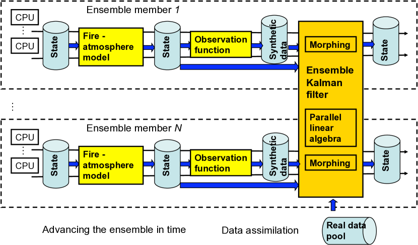
The analysis cycles are run in a shell script loop. Each ensemble member state is maintained in a separate files. The model, the EnKF code, and the evaluation of the observation function are in separate executables, which communicate by files. Each ensemble member runs on a separate group of processors, and the EnKF running on all processors ties them together (Fig. 3).

Running the EnKF and the simulations as a single parallel application with data passed in memory only is also possible, as done [24] for the standalone reaction-diffusion equation fire model. However, running the EnKF and the simulations separately affords more flexibility, does not force integration of the codes into a single executable, and allows for natural checkpointing and restart of the data assimilation scheme.

For efficiency, on computer clusters with local filesystems on nodes, the files with the state of a member should be kept in local files on the nodes used to advance that member. Some computer systems, such as IBM BlueGene, have a single high-performance file system, designed for massively parallel access, with multiple independent high-speed links from subsets of nodes. In that case, simulations running on separate groups of nodes can access their files on the common filesystem without interference with each other.

III Assimilation of data into fire models

Wildfire data is often sparse in space and time and innacuracies in the models and the initial conditions are inevitable. So, the model state can differ significantly from the data that is being assimilated. Yet, the simulation must recover and continue. Thus, an important quality of data assimilation methods is their ability to make large corrections to the state without breaking the assimilation method or the model.

The EnKF applied to either fire model described above fails quickly [4, 8]. One reason is that errors in fire simulations often involve an inaccurate location of the fire. The task of the EnKF to find the best fit to the data is then futile, because the EnKF makes amplitude corrections rather than position corrections.

Another aspect of the failure of the EnKF that the EnKF is based on the assumption that all probability distributions involved are at least approximately Gaussian. While the location of the fire may have an error distribution that is approximately Gaussian, this phenomenon is certainly not the case for the value of the state (such as the temperature) at a given point. Instead, the probability distribution of the state at a given point near the fireline is concentrated around the burning and the not burning states.

Finally, fire models are irreversible and non dissipative, and, consequently, they behave quite differently from the usual atmospheric and oceanic models that EnKF is applied to. The mode of failure of the EnKF for both models is similar. Statistical variability of the EnKF corrections causes spurious fires, which continue burning and may even grow instead of conveniently going away like, e.g., spurious plumes in pollution models, which dissipate readily. In physics based models, such as the reaction-diffusion model described above, the EnKF corrections result in nonphysical states, which cause the model to break down.

III-A Regularized EnKF

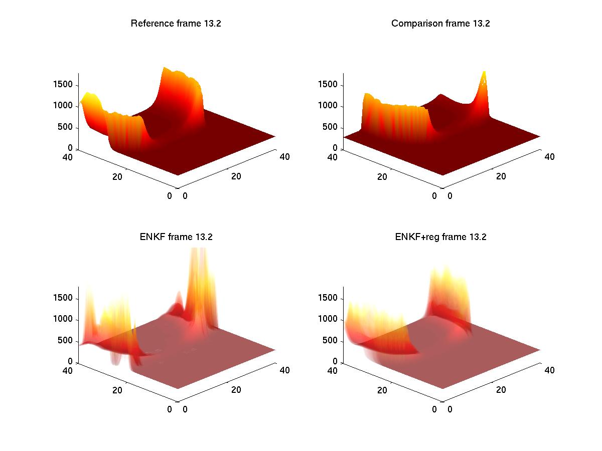
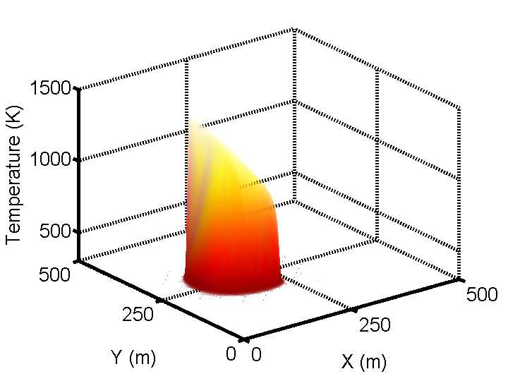
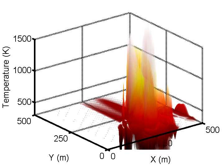
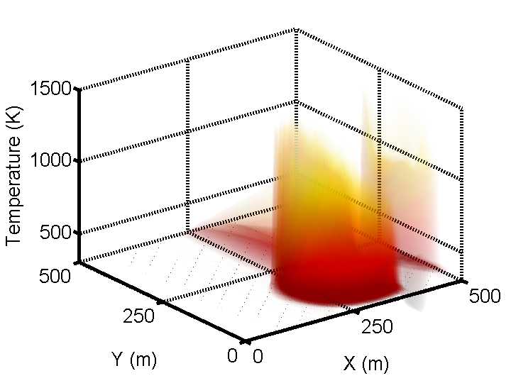
The nonphysical states from the EnKF analysis step in the physics based model are characterized by the values of the physical fields out of bounds, such as the spikes in the temperature field in the lower left panel in Fig. 4. Therefore, it is natural to consider penalizing the large nonphysical values, hoping to stabilize the computation. This approach was tried, but without much success, because the nonphysical values are not all that different from valid ones. However, the spatial gradients in the spikes in the state from EnKF are much larger than the gradients normally seen in a physically reasonable solution. Thus, the regularized EnKF [7] was developed which penalizes large changes in spatial gradients in the Bayesian update. One possible implementation is to add a penalty term involving the norm of the spatial gradients of the solution to the objective function in the minimization formulation of EnKF, much like Tikhonov regularization for ill-posed problems. However, the regularization can be implemented simply by adding an artificial observation $\bigtriangledown u=\bigtriangledown\bar{u}$ to EnKF, where $u$ is one of the fields in model state (such as the temperature), $\bigtriangledown$ is the spatial gradient, computed by finite differences, and $\bar{u}$ is the same field in the mean of the forecast ensemble. The amount of penalty is controlled by the error covariance for the observation; smaller error covariance means stronger penalization of large changes in the gradient. Because the added observation is independent of other data in the Bayesian update, it is easily implemented by running the EnKF formulas twice, thus requiring very little new code.

The regularization technique does have a stabilizing effect on the simulations in the ensemble (Fig. 4), but finding the proper value of the penalty constant is tricky and the regularization does not improve much the ability of the EnKF to track the data. The posterior ensemble is made out of linear combinations of the prior ensemble, and if a reasonably close location and shape of the fire cannot be found between the linear combinations, the data assimilation is simply out of luck, and the ensemble cannot approach the data. From that point on, the ensemble evolves essentially without regard to the data.

III-B Morphing EnKF

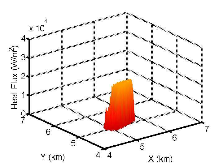
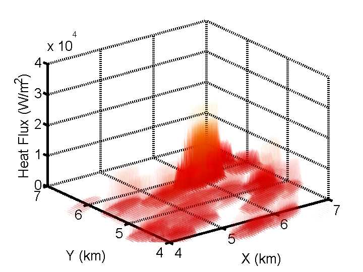
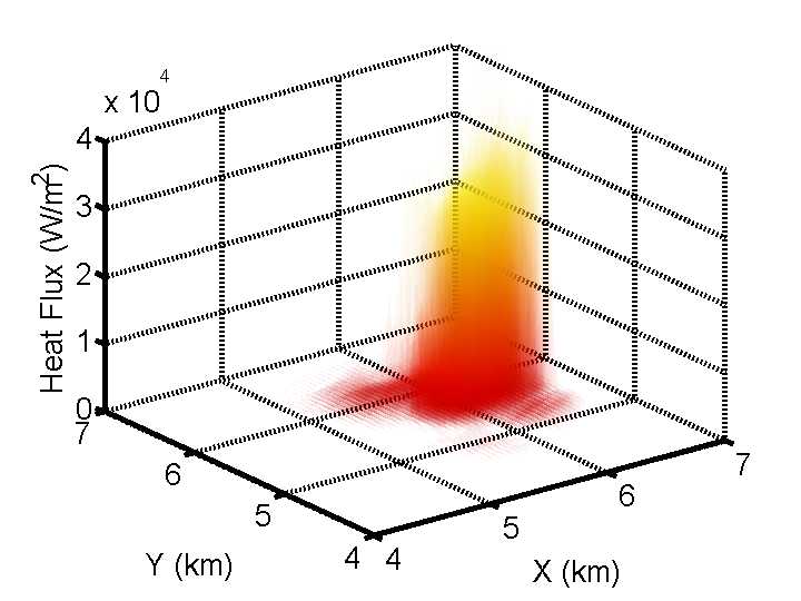
A level set fire spread model makes it possible to manipulate the location of the fire easily by changing the level function just like any other physical field. Yet, the hope that the level set representation of the fire region would be all that would be needed for a succesful fire data assimilation did not pan out: the EnKF causes a number of spurious fires even with the level set model, as seen in the lower left panel in Fig. 7.

There is clearly a need to adjust the simulation state by a change of position explicitly rather than by an additive correction. We use techniques from image processing for this purpose. Moving and stretching one given image to become another given image is known as registration [25]. Classical registration methods require a user to pick which points are to be transformed into which points, but fully automatic methods now exist. Once the two images are registered, one can easily create intermediate images, which is known as morphing. The intermediate images can be created in such a way that they can be used instead of linear combinations of states in EnKF. The resulting method [8] provides both additive and position correction combined in a natural manner. Related methods in the literature include transformation of the space by a low-order polynomial mapping [26] and solving a differential equation to find an alignment mapping as a preprocessing to an additive correction [27, 28].

The basic ingredient in the morphing EnKF is automatic registration, borrowed from image processing. Consider two functions $u_{0}$, $u_{1}$, representing the same physical field, such as the temperature, or the level set function, from two states of a wildfire model. The functions are represented by gridded arrays on the fire problem domain, and considered interpolated away from grid nodes. Let $x=\left(x_{1},x_{2}\right)$ be coordinates of a point in the fire problem domain on the surface of the Earth. The registration problem is to find a mapping $T$ $:x\mapsto T\left(x\right)$ such that the change of variable $x\mapsto x+T\left(x\right)$ transforms $u_{0}$ into a function approximately equal to $u_{1}$, $u_{0}\left(x+T\left(x\right)\right)$ $\approx u_{1}\left(x\right)$. This process can be written in the compact form

$$u_{1}\approx u_{0}\circ\left(I+T\right)\text{ on }D,$$ (15)

where $\circ$ denotes the composition of mappings, and $I:x\mapsto x$ is the identity mapping. The mapping $I+T$ is called the registration mapping, and the mapping $T$ is called warping. The reason for writing the registration mapping as $I+T$ is that the zero warping $T=0$ is the neutral element of the operation of addition, and so linear combinations of warpings have a meaningful interpretation as blends of the warpings.

To avoid unnecessarily large warping, $T$ must be as close to zero and as smooth as possible

$$T\approx 0,\quad\nabla T\approx 0,$$ (16)

where $\nabla T$ denotes the matrix of the first derivatives (the Jacobian matrix) of $T$. In addition, we require that the registration mapping $I+T$ is one-to-one, so that the inverse $\left(I+T\right)^{-1}$ exists. For a fully automatic method to construct such a mapping $T$, see “Image registration.” The mapping $T$ is represented by its values on the grid and interpolated away from the grid points.

Once the registration mapping $I+T$ is found, one can construct intermediate functions $u_{\lambda}$ between $u_{0}$ and $u_{1}$ by the morphing formula [8]

$$u_{\lambda}=\left(u+\lambda r\right)\circ\left(I+\lambda T\right),\quad 0\leq\lambda\leq 1,$$ (17)

where

$$r=u_{1}\circ\left(I+T\right)^{-1}-u_{0}.$$ (18)

The original functions $u_{0}$ and $u_{1}$ are recovered by choosing in (17) $\lambda=0$ and $\lambda=1$. The formula (17) blends naturally the change in position and value. It is more complicated and expensive than alternatives, such as $u_{\lambda}=u_{0}\circ\left(I+\lambda T\right)$, which modifies the position only, or $u_{\lambda}=u_{0}\circ\left(I+\lambda T\right)+\lambda\left(u_{1}-u_{0}\circ\left(I+T\right)\right)$, which combines value and position correction but the value correction is always in a fixed place. However, the results obtained with (18) are much more satisfactory, and the inverse mapping can be evaluated by a fast inverse interpolation: if $y_{i}$ are grid nodes and $x_{i}=\left(I+T\right)y_{i}$, then $y=\left(I+T\right)^{-1}x$ is obtained by interpolating the values of $y_{i}$ on the nonuniform grid formed by $x_{i}$.

The morphing EnKF works by transforming the member states into extended states $\left[r,T\right]$ consisting of additive and position components that encode the difference of the member from some base state $u_{0}$. The EnKF formulas are then run on the extended states $\left[r,T\right]$. Afterwards, the extended states are converted back by (17) and advanced in time. The base state $u_{0}$ can be created by taking the average of the extended states $\left[r,T\right]$ after the EnKF update, transforming back, and advancing in time. Alternatively, the base state can be chosen as one of the ensemble members, or, for short simulation times, the base state may be fixed as the initial state that the ensemble was created from.

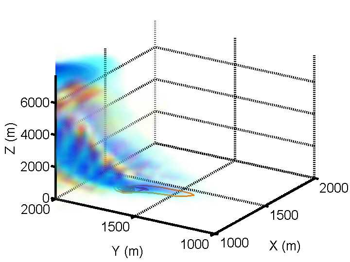
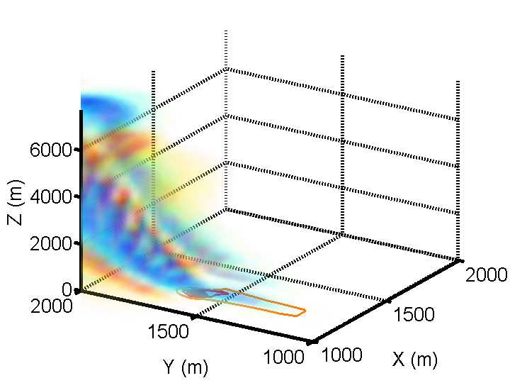
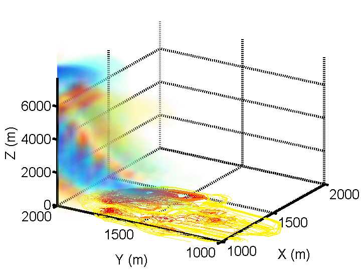
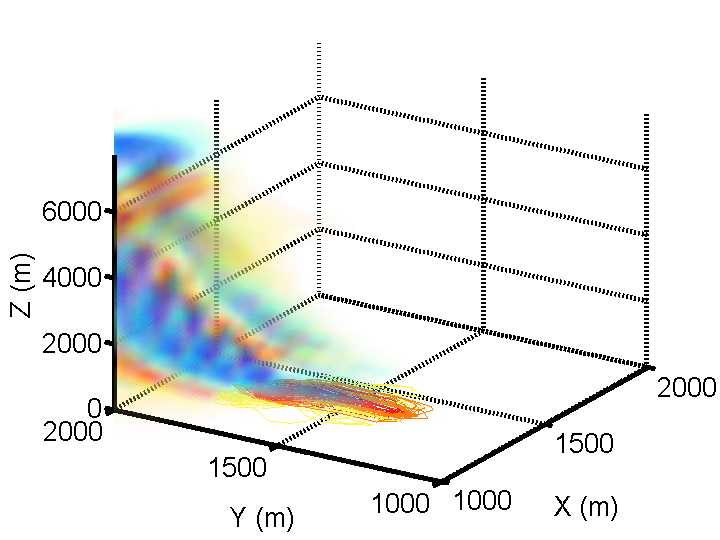
The morphing EnKF has been demonstrated to be capable of making a large correction in the state and tracking the data in an accurate and stable manner for the reaction-diffusion model (Fig. 6) as well as for the level set-based fireline propagation model (Fig. 7) alone or coupled with an atmosphere model (Fig. 8).

IV Conclusion

Two wildland fire models and methods for assimilating data in those models are presented. The EnKF is implemented in a distributed-memory high-performance computing environment. Data assimilation methods are developed combining EnKF with Tikhonov regularization to avoid nonphysical states and with the ideas of registration and morphing from image processing to allow large position corrections. The data assimilation methods can track the data even in the presence of the large correction, and avoid divergence. The methods can assimilate gridded data, but the assimilation of station data and steering of data acquisition is left to future developments.

A semi-empirical fire spread model is implemented by the level set model and coupled with the Weather Research Forecasting (WRF) model. The coupled fire-atmosphere code is distributed with the WRF download as of Spring 2009, and it is also available directly from the authors.

V Acknowledgments

This work is a part of an effort to build a Dynamic Data Driven Application System (DDDAS) [29] for wildland fire prediction, funded by the National Science Foundation (NSF). This research was partially supported by NSF grants CNS-0325314, CNS-0324910, CNS-0719641, DMS-0623983, ATM-0835579, and ATM-0835598, and by the National Center for Atmospheric Research (NCAR) Faculty Fellowship.

Computer time on IBM BlueGene/L supercomputer was provided by NSF MRI Grants CNS-0421498, CNS-0420873, and CNS-0420985, NSF sponsorship of the NCAR, the University of Colorado, and a grant from the IBM Shared University Research (SUR) program.

The authors would like to thank Craig Douglas, Deng Li, Wei Li, and Adam Zornes from the University of Kentucky for their contributions to the software infrastructure that some of the codes used here are built on, John Michalakes from NCAR for his assistance with WRF, and Ned Patton from NCAR for providing his prototype code for interfacing an earlier fireline propagation model with WRF.

VI Author Information

Jan Mandel is Professor of Mathematical and Statistical Sciences and Adjunct Professor of Computer Science and Engineering at the University of Colorado Denver, Denver, CO, and visiting scientist at the National Center for Atmospheric Research, Boulder, CO, email Jan.Mandel@cudenver.edu. He received his PhD in Numerical and Approximate Methods from the Charles University, Prague, Czech Republic, in 1983. He has developed domain decomposition and multilevel iterative solvers for large problems of equations from finite elements. He is interested in high-performance computing, wildfire modeling, and the development and probabilistic analysis of data assimilation methods.

Jonathan D. Beezley is a PhD student of Applied Mathematics at the University of Colorado Denver and visiting graduate student at the National Center for Atmospheric Research, Boulder, CO. He is interested in ensemble filters, parallel software, and image registration.

Janice L. Coen is a project scientist at the National Center for Atmospheric Research, Boulder, CO. She received a PhD in Geophysical Sciences from the University of Chicago in 1992. Her interests are in mesoscale meteorology and wildland fire behavior. She has developed components of a coupled atmosphere-fire model and led the implementation of an operational weather forecasting system for the United Arab Emirates.

Minjeong Kim is a PhD student of Applied Mathematics at the University of Colorado Denver. She is interested in numerical schemes for level set methods and in wildfire modeling by partial differential equations.

Figure 1: An example of reaction heat balance function $h(T)$ from modified Arrhenius reaction dynamics with cooling (1). The three zeros of the function, in increasing order, are the ambient temperature $T_{a}$, the auto-ignition temperature $T_{i}$, and the high burning temperature $T_{c}$. For the temperature $T$ between $T_{a}$ and $T_{i}$, the heat produced by the reaction is less than the heat loss by cooling. Once the $T$ higher than the $T_{i}$, but less than $T_{c}$, the reaction heat is more than the heat loss by cooling, and fire results. Thus, $T_{i}$ is unstable equilibrium. Since the heat loss by cooling grows linearly with the temperature but the reaction rate is bounded, for high enough temperature, $T>T_{c}$, the heat loss by cooling prevails. Reproduced from [4].

Figure 2: Measured and computed temperature as the fire passes over a sensor in a fixed location. The measured time-temperature profile (dash line) in a grass wildland fire is digitized from [30]. The computed computed profile (solid line) is obtained from a simulation by a numerical solution of the reaction-diffusion equations (1) – (4). The model was ignited by raising the temperature in a subinterval, then two waves develop traveling away from the ignition and eventually stabilize. The computed profile shows such wave, traveling to the left. Reproduced from [4].

Figure 3: Parallel ensemble management scheme. In each cycle, all ensemble members are advanced in time, each member by a separate run of the simulation code. The simulation code is a parallel application, which executes on a collection of processors, both for speed and distribution of the memory use. When enough processors are available, some or all ensemble members are advanced concurrently. After all ensemble members are advanced in time, the value of the observation function is evaluated for each ensemble member and the EnKF code is started on all available nodes. The EnKF code loads the state of the ensemble members and the values of the observation function from the files, reads the data to be assimilated from data files, and performs the analysis calculations using high-performance parallel linear algebra. The modified states of ensemble members are written to files and the cycle repeats.

Figure 4: Example of the effect of regularization by penalization of large change in gradients by the Bayesian update on propagation of fire. Circular spreading fire hits a fuel break in the middle of the domain. The horizontal axes are distance in m. The vertical axis is temperature in K. False color is generated from the temperature with shading for depth perception. The reference solution is the simulated data. In the comparison solution, the fire was started from intentionally incorrect location. The ENKF panel is the result of data assimilation after 13 cycles. The ENKF+reg panel is the ensemble after data assimilation after 13 cycles with regularization imposed in each cycle. The ensembles have 100 members and they are visualized as superposition of transparent images of their members. The observation function was the temperature field on the whole grid. Both ensembles succeed in moving toward the data, but the regularized ensemble avoids the non-physical artefacts, such as extremely small and large temperatures.

$\lambda=0$	$\lambda=0.25$	$\lambda=0.5$	$\lambda=0.75$	$\lambda=1$

Figure 5: Morphing of two solutions of a reaction-diffusion equation system (1) – (4) used in a wildfire simulation. The states with $\lambda=0$ and $\lambda=1$ are given. The intermediate states with $0<\lambda<1$ are created automatically by the morphing algorithm (17). The horizontal plane is the earth surface. The vertical axis and the color map are the temperature. The morphing algorithm combines the values as well as the positions. Reproduced from [8].

(a)	(b)
(c)	(d)

Figure 6: The morphing EnKF applied to the reaction-diffusion model (1) – (4). False color is generated from the temperature with shading for depth perception. The reference solution (a) is the simulated data. The initial ensemble was created by a random perturbation of the comparison solution (b), where the fire was ignited at an intentionally incorrect location. The standard ENKF panel (c) is the result of data assimilation of the temperature field after running the model for 500 seconds. The morphing EnKF panel (d) is the ensemble with the image registration against the temperature field at the time of ignition, and applied to both the temperature and the fuel supply. The ensembles have 25 members each and they are visualized as superposition of transparent images of their members. The observation function was the temperature field on the whole grid. The standard EnKF ensembles diverges from the data, while the morphing EnKF ensemble keeps closer to the data.

(a)	(b)
(c)	(d)

Figure 7: The morphing EnKF applied to the fireline propagation model. False color is the output heat flux with shading for depth perception. The reference solution (a) is the simulated data. The initial ensemble was created by a random perturbation of the comparison solution (b), where the fire was ignited at an intentionally incorrect location. The standard ENKF panel (c) is the result of data assimilation of the time from ignition after running the model for 1000 seconds. The morphing EnKF panel (d) is the result with image registration determined from the time from ignition and applied to all of the model variables. The ensembles have 25 members each and they are visualized as superposition of transparent images of heat fluxes of their members. The registration was done on the atmospheric grid with the fire heat flux as the observation function, but the atmospheric model was not used. The standard EnKF ensembles diverges from the data, while the morphing EnKF ensemble keeps closer to the data.

(a)	(b)
(c)	(d)

Figure 8: The morphing EnKF applied to the fireline propagation model coupled with WRF. False color and contour on the horizontal plane is the output heat flux. The volume shading is the vorticity of the atmosphere where red and blue shades represent positive and negative vorticity, respectively. A contour plot of the heat flux due to the fire is shown on the x-y plane. The reference solution (a) is the simulated data. The initial ensemble was created by a random perturbation of the comparison solution (b), with the fire ignited at an intentionally incorrect location. The standard ENKF (c) and the morphing EnKF (d) were applied after 15 minutes. The ensembles have 25 members each. Shown are the mean vorticity and the superposition of the heat fluxes in ensemble members. The registration was done on the atmospheric grid with the fire heat flux as the observation function. The standard EnKF ensembles diverges from the data, while the morphing EnKF ensemble keeps closer to the data.

Sidebar - Wildland Fire Modeling

The purpose of wildland fire modeling is to understand and ultimately predict fire behavior in order to increase safety of firefighters and the public, to reduce risk and minimize damage, and to protect ecosystems, watersheds, and air quality.

VI-A What is fire modeling?

The process of fire modeling aims to reproduce and anticipate properties of fire behavior and fire effects. Fire behavior includes the rate of spread of the flaming front (the interface between burning and unburned fuel), the heat release rate which is related to the burning intensity, as well as specific phenomena such as the bending forward of the fire front, transition from surface to crown fires, and extreme fire activity such as firewhirls. Fire effects which include ecological and hydrological effects on the landscape, such as the percentage of forest fuel consumed in prescribed fires, mortality suffered by trees, or the quantity of smoke produced for health impacts.

Three environmental factors affect wildland fire behavior: weather, fuel characteristics, and topography. Fuel factors include the type, moisture, size, shape, amount, and arrangement. Topography factors include the orientation toward the sun, the slope, and features such as narrow canyons and barriers such as creeks, roads, and unburnable fuel. Of the three environmental factors, weather (including factors such as wind, temperature, relative humidity, and precipitation) is the most rapidly changing. Weather phenomena that bring changes such as cold fronts, foehn winds, thunderstorm downdrafts, sea and land breezes, and diurnal slope winds can be particularly dangerous, since they can suddenly change the fire’s direction and behavior. Weather also influences wildfires through the other factors of fuel and topography, by controlling the fuel moisture through precipitation, RH, and winds, and by complicating the fire-accelerating effect of slopes with topographically-induced accelerations. These factors are not independent. Weather and terrain combine to produce topographic effects such as downslope windstorms (called Santa Annas, foehn winds, East winds, depending on the geographic location), the weather influences fuel moisture as dry winds or precipitation increases or decreases evaporation of moisture and therefore the fuel moisture, and fuel properties may vary with topography as plant density varies with elevation or aspect with respect to the sun. Although weather can influence wildfire behavior through many pathways, it has long been recognized that fires “create their own weather”. That is, the heat and moisture created by the fire feed back into the atmosphere, creating intense winds that drive the fire’s behavior, sometimes overwhelming the effect of ambient winds.

VI-B Approaches to fire modeling

Wildland fire models span a vast range of complexity, from simple cause and effect principles to the most physically complex presenting a difficult supercomputing challenge that cannot hope to be solved faster than real time. Conceptual models from experience and intuition from past fires can be used to anticipate the future. Many semi-empirical fire spread equations as in [11], [S1], and [S2] and [S3] for Australasian fuel complexes have been developed for quick estimation of fundamental parameters of interest such as fire spread rate, flame length, and fireline intensity of surface fires at a point for specific fuel complexes, assuming a representative point-location wind and terrain slope. Based on the work in [S4] and [S5] the quasi-steady equilibrium spread rate calculated for a surface fire on flat ground in no-wind conditions was calibrated using data of piles of sticks burned in a flame chamber/wind tunnel to represent other wind and slope conditions for the fuel complexes tested. A simplified physically-based two-dimensional fire spread model based upon conservation laws that use radiation as the dominant heat transfer mechanism and convection, which represents the effect of wind and slope was developed in [S6]. Two-dimensional fire growth models such as FARSITE [S7] and Prometheus, the Canadian wildland fire growth model designed to work in Canadian fuel complexes, have been developed that apply such semi-empirical relationships and others regarding ground-to-crown transitions to calculate fire spread and other parameters along the surface. Certain assumptions must be made in models such as FARSITE and Prometheus to shape the fire growth for example, Prometheus and FARSITE use the Huygens principle of wave propagation. A set of equations that can be used to propagate (shape and direction) a fire front using an elliptical shape was developed in [S8]. Although more sophisticated applications use a three-dimensional numerical weather prediction system to provide inputs such as wind velocity to one of the fire growth models listed above, the input was passive and the feedback of the fire upon the atmospheric wind and humidity are not accounted for.

More complex physical models join computational fluid dynamics models with a wildland fire component and allow the fire to feed back upon the atmosphere. These models include NCAR’s Coupled Atmosphere-Wildland Fire-Environment (CAWFE) model developed in [S9], Los Alamos National Laboratory’s FIRETEC developed in [S10], and the WUI (Wildland Urban Interface) Fire Dynamics Simulator (WFDS) [S11] and, to some degree, the two-dimensional model PIF97 [S12, S13]. These tools have different emphases and have been applied to better understand the fundamental aspects of fire behavior, such as fuel inhomogeneities on fire behavior [S10], feedbacks between the fire and the atmospheric environment as the basis for the universal fire shape [S14, 5], and are beginning to be applied to wildland urban interface house-to-house fire spread at the community-scale. The cost of added physical complexity is a corresponding increase in computational cost, so much so that a full three-dimensional explicit treatment of combustion in wildland fuels by direct numerical simulation (DNS) at scales relevant for atmospheric modeling does not exist, is beyond current supercomputers, and does not currently make sense to do because of the limited skill of weather models at spatial resolution under $1$ km. Consequently, even these more complex models parameterize the fire in some way, for example, [S15, S16] use [11] to calculate local fire spread rates using fire-modified local winds. And, although FIRETEC and WFDS carry prognostic conservation equations for the reacting fuel and oxygen concentrations, the computational grid cannot be fine enough to resolve the reaction rate-limiting mixing of fuel and oxygen, so approximations must be made concerning the subgrid-scale temperature distribution or the combustion reaction rates themselves. These models also are too small-scale to interact with a weather model, so the fluid motions use a computational fluid dynamics model confined in a box much smaller than the typical wildfire. The limitations on fire modeling are not entirely computational. At this level, the models encounter limits in knowledge about the composition of pyrolysis products and reaction pathways, in addition to gaps in basic understanding about some aspects of fire behavior such as fire spread in live fuels and surface-to-crown fire transition.

Thus, while more complex models have value in studying fire behavior and testing fire spread in a range of scenarios, from the application point of view, FARSITE and Palm-based applications of BEHAVE have shown great utility as practical in-the-field tools because of their ability to provide estimates of fire behavior in real time. While the coupled fire-atmosphere models have the ability to incorporate the ability of the fire to affect its own local weather, and model many aspects of the explosive, unsteady nature of fires that cannot be incorporated in current tools, it remains a challenge to apply these more complex models in a faster-than-real-time operational environment. Also, although they have reached a certain degree of realism when simulating specific natural fires, they must yet address issues such as identifying what specific, relevant operational information they could provide beyond current tools, how the simulation time could fit the operational time frame for decisions (therefore, the simulation must run substantially faster than real time), what temporal and spatial resolution must be used by the model, and how they estimate the inherent uncertainty in numerical weather prediction in their forecast. These operational constraints must be used to steer model development.

Sidebar - Level Set-Based Wildland Fire Model

VI-C Curve propagation by the level set method

Consider a curve $\Gamma=\Gamma\left(t\right)$ in $\mathbb{R}^{2}$ evolving with the speed $S\left(x,t\right)$ in the normal direction. The level set method represents the curve as the level set

$$\Gamma=\left\{x:\psi\left(x,t\right)=0\right\}$$

of a function $\psi$, called a level set function, and converts the evolution of the curve into a differential equation for the level set function, which is then solved numerically. In applications, the curve $\Gamma$ is closed, and we choose that the inside of the curve is given by $\psi<0$. Because $\psi=0$ on $\Gamma$, the component of $\nabla\psi$ in the tangent direction is zero, and so $\nabla\psi$ has the normal direction to $\Gamma$. Thus, we can also use the level set function $\psi$ to compute the normal to the curve $\Gamma$ by

$$\overrightarrow{n}=\frac{\nabla\psi}{\left\|\nabla\psi\right\|},$$

where $\left\|\cdot\right\|$ is the Euclidean norm.

To derive an equation to evolve the level set function, consider a point $x=x\left(t\right)\in\Gamma\left(t\right)$. Then $\psi\left(x\left(t\right),t\right)=0$, and from the chain rule

$$0 =\frac{d}{dt}\psi\left(x,t\right)$$

$$=\frac{\partial\psi}{\partial t}+\underbrace{\nabla\psi}_{\left\|\nabla\psi\right\|\overrightarrow{n}}\cdot\frac{\partial x}{\partial t}$$

$$=\frac{\partial\psi}{\partial t}+\left\|\nabla\psi\right\|\underbrace{\overrightarrow{n}\cdot\frac{\partial x}{\partial t}}_{S\left(x\right)}.$$

Thus, the level set function is governed by the partial differential equation, called the level set equation [S17] [S18, Ch. 1]

$$\frac{\partial\psi}{\partial t}+S\left(x\right)\left\|\nabla\psi\right\|=0.$$

Note that the level set equation requires propagation speed $S\left(x\right)$ to be defined at all points $x$, not just on the curve $\Gamma$, even if the curve propagation itself depends only on the speed $S$ given on $\Gamma$.

One example of the level set function is the signed distance function

$$\psi\left(x\right)=\pm\operatorname*{dist}(x,\Gamma),$$

with $-$ inside and $+$ outside of $\Gamma$. The signed distance function is characterized by $\left\|\nabla\psi\right\|=1$. Ideally, $\psi$ should be equal or close to the signed distance function for numerical stability, but this property is in general not preserved when advancing the level set equation in time.

Since in the wildland fire model here always $S\geq 0$, the level set function does not increase with time and the fire area cannot decrease (Fig. S1).

VI-D Numerical solution of the level set equation

The spread rate $S$ is defined by the Rothermel formula (5) at every point, not only the fireline. Thus, the fuel data and wind over the whole domain can be used to propagate the level set function, avoiding the problem how to extend the speed from the fireline. The level set equation is discretized on a rectangular grid rectangular mesh with spacing $\left[\triangle x_{1},\triangle x_{2}\right]$. To advance the model in time, the Runge-Kutta method of order $2$ (Heun’s method) is used,

$$\psi^{n+1/2}=\psi^{n}+\Delta tF\left(\psi^{n}\right),\quad\psi^{n+1}=\psi^{n}+\Delta t\left(\left(1-\alpha\right)F\left(\psi^{n}\right)+\alpha F\left(\psi^{n+1/2}\right)\right),\quad\alpha=\frac{1}{2}.$$

The right-hand side $F$ is a discretization of the term $-S\left\|\nabla\psi\right\|$ with upwinding and artificial viscosity,

$$F\left(\psi\right)=-S\left(\overrightarrow{v}\cdot\overrightarrow{n},\nabla z\cdot\overrightarrow{n}\right)\left\|\overline{\nabla}\psi\right\|+\varepsilon\triangle\psi,\quad\overrightarrow{n}=\nabla\psi/\left\|\nabla\psi\right\|,$$

where $\overline{\nabla}\psi=\ \left[\overline{\nabla}_{1}\psi,\overline{\nabla}_{2}\psi\right]$ is the upwinded approximation of the gradient of $\psi$ by the Godunov method [S19, p. 58],

$$\overline{\nabla}_{1}\psi=\left\{\begin{tabular}[c]{ll}$\nabla_{1}^{-}\psi$,&if $\nabla_{1}^{-}\psi\geq 0$ and $\nabla_{1}^{-}\psi+\nabla_{1}^{+}\psi\geq 0,$\\ $\nabla_{1}^{+}\psi$,&if $\nabla_{1}^{+}\psi\leq 0$ and $\nabla_{1}^{-}\psi+\nabla_{1}^{+}\psi<0$,\\ $0$,&otherwise,\end{tabular}\ \ \right.$$

where $\nabla_{1}^{+}\psi$ and $\nabla_{1}^{-}\psi$ are the right and the left one-sided numerical derivatives

$$\nabla_{1}^{+}\psi\left(x_{1},x_{2}\right) =\frac{\psi\left(x_{1}+\triangle x_{1},x_{2}\right)-\psi\left(x_{1},x_{2}\right)}{\triangle x_{1}},$$

$$\nabla_{1}^{-}\psi\left(x_{1},x_{2}\right) =\frac{\psi\left(x_{1},x_{2}\right)-\psi\left(x_{1}-\triangle x_{1},x_{2}\right)}{\triangle x_{1}},$$

and similarly for $\nabla_{2}^{+}\psi$ and $\nabla_{2}^{-}\psi$. Further,

$$\nabla\psi=\left[\frac{\nabla_{1}^{+}\psi+\nabla_{1}^{-}\psi}{2},\frac{\nabla_{2}^{+}\psi+\nabla_{2}^{-}\psi}{2}\right]$$

is the gradient by central differences, $\varepsilon$ is the scale-free artificial viscosity ($\varepsilon=0.4$ in the computations here), and

$$\triangle\psi=\left(\nabla_{1}^{+}\psi-\nabla_{1}^{-}\psi+\nabla_{2}^{+}\psi-\nabla_{2}^{-}\psi\right)$$

is the scaled five-point Laplacian of $\psi$. The wind velocity $\overrightarrow{v}\left(x\right)$ can be evaluated at $x-d\overrightarrow{n}$ instead, i.e., at the fireline, the winds are taken from the distance $d$ behind the fireline.

The use of a numerically stable scheme that includes upwinding, such as the Godunov scheme above in the norm of the gradient, is required; when the gradient there is approximated by standard central differences, the numerical method fails quickly. However, it seems better to use central differences in the computation of the normal $\overrightarrow{n}$.

The reason for using Heun’s method is not accuracy but conservation. In numerical computations, the second time derivative of the level set function tends be negative, $\partial^{2}\psi/\partial^{2}t<0$, and so the explicit Euler method ($\alpha=0$ above) tends to systematically overestimate $\psi$ and thus fire propagation slows down or stops altogether. Similarly, the choice $\alpha=1$ tends to systematically underestimate $\psi$. Heun’s method ($\alpha=1/2$) as the average of the two behaves reasonably well.

VI-E Boundary conditions

Before computing the one-sided differences up to the boundary, the level set function is extrapolated to one layer of nodes beyond the boundary. However, the extrapolation is not allowed to decrease the value of the level set function under the value at the boundary. For example, when $\left(n,k\right)$ is the last node in the domain in the direction $x_{1},$ the extrapolation

$$\psi_{n+1,k}=\max\left\{\psi_{nk}+\left(\psi_{nk}-\psi_{n-1,k}\right),\psi_{nk},\psi_{n-1,k}\right\},$$

is used, and similarly in other cases. This modification of the finite difference method serves to avoid numerical instabilities at the boundary. The extrapolation at the boundary effectively implements a free boundary condition. Without the stabilization, a decrease of the level set function at boundary node, e.g., due to nonhomogeneity of the fuel, would be amplified by the extrapolation, and, in combination with the effect of the Godunov formula, might cause large negative spikes to develop at the boundary.

VI-F Updating ignition time

The ignition time $t_{i}$ in the strip that the fire has moved over in one timestep is computed by linear interpolation from the level set function. Suppose that the point $x$ is not burning at the time $t$ but it is burning at the time $t+\triangle t$, that is, $\psi\left(x,t\right)>0$ and $\psi\left(x,t+\triangle t\right)\leq 0$. The ignition time $t_{i}\left(x\right)$ at the point $x$ satisfies $\psi\left(x,t_{i}\right)=0$. Approximating $\psi$ linearly in $t$, we have

$$\frac{\psi\left(x,t\right)}{t_{i}\left(x\right)-t}\approx-\frac{\psi\left(x,t+\triangle t\right)}{t_{i}\left(x\right)-\left(t+\triangle t\right)},$$

which gives

$$t_{i}(x)\approx t+\frac{\psi\left(x,t\right)\triangle t}{\psi\left(x,t\right)-\psi\left(x,t+\triangle t\right)}.$$

VI-G Computation of fuel burned

The fuel burned and thus the heat generated are then computed by numerical quadrature over each fire mesh cell from the postulated exponential fuel decay (6). This is a challenging task because the numerical quadrature needs to be able to handle two extreme cases. When the fuel burns slowly relative to the time the fireline takes to cross the cell, the integrand is well approximated by a linear function and the proportion of the fuel burned is related to the volume of the burning area. On the other hand, when the fuel burns quickly relative to the time step and the fireline moves slowly relative to the mesh step size, the fuel burned in one timestep is related to the area of a strip through which the fireline travels during the time step, and asymptotically to the length of the fireline in the cell.

The level set function $\psi$ and the ignition time $t_{i}$ are interpolated to the corners of subcells that form at least twice finer grid. On each subcell $C$, the fuel fraction burned

$$\frac{1}{\operatorname*{area}\left(C\right)}{\displaystyle\iint\limits_{x\in C:\psi\left(x\right)\leq 0}}\left(1-e^{-\frac{t-t_{i}}{T}}\right)dx_{1}dx_{2}$$

is approximated from the values $\psi$ and $t_{i}$ at the corners of the subcell. The fraction of the cell that is burning is approximated by

$$\operatorname*{area}\left\{x\in C:\psi\left(x\right)\leq 0\right\}\approx\beta=\frac{1}{2}\left(1-\frac{\sum_{k=1}^{4}\psi_{k}}{\sum_{k=1}^{4}\left|\psi_{k}\right|}\right),$$

where $\psi_{1},\ldots,\psi_{4}$ are the values of the level set function at the corners of the subcell. The approximation is exact in several important cases: No part of the cell is on fire, all $\psi_{k}\geq 0$ and at least one $\psi_{k}>0$, then $\beta=0$; the whole cell is on fire, all $\psi_{k}\leq 0$ and at least one $\psi_{k}<0$, then $\beta=1$; or the values $\psi_{k}$ define a linear function and the fireline crosses the cell diagonally or it is aligned with one coordinate direction.

Next, replace the time from ignition on the subcell corners by zero whenever the level set function is positive (then the corner cannot be on fire), and compute the approximate fraction of the fuel burned as $\beta\left(1-e^{-t_{a}/W}\right)t_{a}$, where $W$ is the time constant of the fuel in the cell and $t_{a}$ is the average of the modified time from ignition on the subcell corners. This computation is a second-order quadrature formula when the whole cell is burning, accurate when no part of the cell is burning, and it provides a natural transition between the two. Also, the calculation is accurate asymptotically when the fuel burns slowly and the approximation $\beta$ of the burning area is exact. However, a rigorous investigation of the accuracy of the quadrature is beyond the scope of this paper.

VI-H Ignition

The model is initialized with no fire by choosing the level set function $\psi\left(x\right)=1$. If a given ignition time $t_{0}$ falls within the time step, then the level set function is multiplied by a function that is negative in the fire region, before entering the time step. For ignition in a circle of radius $r$ around a point $y$, the level set function $\psi\left(x\right)$ is replaced by

$$\left(\left\|x-y\right\|-r\right)\psi\left(x\right),$$

Ignition within radius $r$ of a more general object, such as a line $L$, is implemented by replacing the level set function by

$$\left(d\left(x,L\right)-r\right)\psi\left(x\right)$$

where $d\left(x,L\right)$ is the Euclidean distance of the point $x$ from $L$. To avoid discretization artefacts, the ignition radius should be several mesh sizes large.

The ignition time on newly ignited nodes is currently set to the current time $t_{0}$. Alternatively, the ignition time could be initialized to

$$t_{i}\left(x\right)=t_{0}+R_{0}\left(\left\|x-x_{0}\right\|-s\right),\quad\left\|x-x_{0}\right\|\leq s,$$

which gives the time of ignition $t_{0}$ at the boundary of the circle and $t_{0}-R_{0}s$ at the center.

VI-I Related work

One problem with level set methods is that they do not guarantee the a-priori conservation of the shape or volume of the level set even in a uniform constant velocity field. Because of the numerical dispersion inherent in upwinding schemes, the shape of level set function flattens up and the level set may either grow too much or decrease and eventually vanish. Also, details of the level set get smeared, and the level set gets seriously distorted, e.g., in a rotational velocity field. For this reason, high-order essentially non-oscillatory (ENO) finite differences in space and high-order Runge-Kutta methods in time are recommended [S17] [S18, Ch. 1] and indeed required in, e.g., the code from [S21]. In addition, sophisticated approaches have been developed to improve the conservation of the level set, such as the hybrid particle level set method [S22], quadrature-free discontinuous Galerkin method [S23], and flux-based level set method [S24].

However, the condition that the fire always spreads forward by a minimum backing rate $B_{0}\geq 0$, and thus the level set function can only decrease, appears to prevent numerical artefacts in the fire model. The much simpler Godunov upwinding and the second-order Runge-Kutta method along with the stabilizations described above are sufficient in the computations reported here.

In [S20], the narrow band level set method with velocity extension from the nearest point on the fireline was used to implement the fireline propagation model from [S21]. The model postulates different spread rates at the head and the flanks of a fire and it does not consider the fuel balance or a coupling with the atmosphere. The narrow band level set method maintains only the values of the level set function in a band along the fireline. It can save a large number of operations and it may reduce the tendency of level set methods to distort the fire area, because the pieces of the level set function emanating from different parts of the fireline do not need to be reconciled globally. However, a narrow band level set method does not seem to be as suitable for data assimilation, it does not fit naturally in the framework of geophysical codes, which operate on rectangular arrays, and the level set method as described above seems to be satisfactory.

Sidebar - Image Registration

Moving and stretching one given image to become another given image is known in image processing as registration [25]. The procedure outlined here can do that fully automatically, without a human intervention.

Given function $u$ and $v$ on a domain $D$, the registration problem can be formulated as

$$v\approx u\circ\left(I+T\right)\text{ on }D.$$

At the same time, we wish that $T$ and $\bigtriangledown T$ are not unnecessarily large. These requirements naturally lead to a construction of the mapping $T$ by optimization

$$J(T)=\|v-u\circ\left(I+T\right)\|+C_{1}\|T\|+C_{2}\|\bigtriangledown T\|\rightarrow\min_{T},$$

where $\|\cdot\|$ are suitable norms. We choose the $L^{1}\left(D\right)$ norms, $\|v\|=\int_{D}\left|v\right|dx$, evaluated by simple numerical integration. To define $\|T\|$ and $\|\bigtriangledown T\|$, we add the norms of the entries of the vector function $T$ and the matrix function $\bigtriangledown T$.

The optimization formulation tries to balance the conflicting objectives of good approximation by the registered image, and as small and smooth warping as possible. The objective function $J(T)$ is in general not a convex function of $T$, and there can be many local minima. For example, a local minimum may occur when some small part of $u$ and $v$ matches, while the overall match is still not good.

The optimization problem for the mapping $T$ is solved by the algorithm from [S25] with some modifications. The method proceeds by building the mapping $T$ on a nested hierarchy of meshes, starting with a coarse mesh that divides the domain $D$ into just four rectangular cells. The mapping $T$ is interpreted as the movement of grid nodes, and the nodes are moved one at a time to minimize a coarse version of $J\left(T\right)$. For each node, a mesh of a number of possible locations is constructed, all locations on the mesh are tested, then the location with the smallest value of $J(T)$ is selected and further improved by a standard descent method. In the coarse version of $J\left(T\right)$, the mapping $T$ is interpolated from the nodes of the current grid, and the functions $u$ and $v$ are smoothed by a convolution to smear fine features and allow a more global match. The resulting mapping is then interpolated to a mesh that is twice finer, and the process continues. See [8] for further details.

Figure S1: The fireline and level set function for a circular fire propagating in constant wind. The fire is in the area where the level set function is negative. The black contour is the fireline. The fire starts at the back of the domain and propagates diagonally until it leaves the domain.

References

- [1] E. Kalnay, Atmospheric Modeling, Data Assimilation and Predictability. Cambridge University Press, 2003.
- [2] G. Evensen, Data assimilation: The ensemble Kalman filter. Berlin: Springer, 2007.
- [3] A. Doucet, N. de Freitas, and N. Gordon, Eds., Sequential Monte Carlo in Practice. Springer, 2001.
- [4] J. Mandel, L. S. Bennethum, J. D. Beezley, J. L. Coen, C. C. Douglas, M. Kim, and A. Vodacek, “A wildland fire model with data assimilation,” Mathematics and Computers in Simulation, vol. 79, pp. 584–606, 2008.
- [5] T. L. Clark, J. Coen, and D. Latham, “Description of a coupled atmosphere-fire model,” Intl. J. Wildland Fire, vol. 13, pp. 49–64, 2004.
- [6] WRF Working Group, “Weather Research Forecasting (WRF) Model,” 2005, http://www.wrf-model.org.
- [7] C. J. Johns and J. Mandel, “A two-stage ensemble Kalman filter for smooth data assimilation,” Environmental and Ecological Statistics, vol. 15, pp. 101-110, 2008.
- [8] J. D. Beezley and J. Mandel, “Morphing ensemble Kalman filters,” Tellus, vol. 60A, pp. 131–140, 2008.
- [9] D. A. Frank-Kamenetskii, Diffusion and heat exchange in chemical kinetics. Princeton University Press, 1955.
- [10] P. Grindrod, The theory and applications of reaction-diffusion equations: Patterns and waves., 2nd ed., Oxford University Press, 1996.
- [11] R. C. Rothermel, “A mathematical model for predicting fire spread in wildland fires,” January 1972, USDA Forest Service Research Paper INT-115.
- [12] T. L. Clark and W. D. Hall, “On the design of smooth, conservative vertical grids for interactive grid nesting with stretching,” J. Appl. Meteor., vol. 35, pp. 1040–1046, 1996.
- [13] J. L. Coen, S. Mahalingam, and J. W. Daily, “Infrared imagery of crown-fire dynamics during FROSTFIRE,” J. Appl. Meteor., vol. 43, pp. 1241–1259, 2004.
- [14] J. Mandel, “Efficient implementation of the ensemble Kalman filter,” CCM Report 231, University of Colorado Denver, 2006. [Online]. Available: http://www.math.cudenver.edu/ccm/reports/rep231.pdf
- [15] B. D. O. Anderson and J. B. Moore, Optimal filtering. Englewood Cliffs, N.J.: Prentice-Hall, 1979.
- [16] G. Burgers, P. J. van Leeuwen, and G. Evensen, “Analysis scheme in the ensemble Kalman filter,” Monthly Weather Review, vol. 126, pp. 1719–1724, 1998.
- [17] G. H. Golub and C. F. V. Loan, Matrix Computations. Johns Hopkins Univ. Press, 1989, second Edition.
- [18] E. Anderson, Z. Bai, C. Bischof, S. Blackford, J. Demmel, J. Dongarra, J. Du Croz, A. Greenbaum, S. Hammarling, A. McKenney, and D. Sorensen, LAPACK Users’ Guide, 3rd ed. Philadelphia, PA: Society for Industrial and Applied Mathematics, 1999.
- [19] J. Dongarra and L. S. Blackford, “Scalapack tutorial,” in Applied Parallel Computing: Industrial Computing and Optimization (Proceedings of the Third Int. Workshop PARA’96, Lyngby, Denmark), J. Wasniewski, J. Dongarra, K. Madsen, and D. Olsen, Eds. Heidelberg: Springer Verlag, 1996, pp. 204–215, http://www.netlib.org/utk/papers/scalapack-tutorial.ps.
- [20] C. L. Keppenne and M. M. Rienecker, “Initial testing of a massively parallel ensemble Kalman filter with the Poseidon isopycnal ocean general circulation model,” Monthly Weather Review, vol. 130, pp. 2951–2965, 2002.
- [21] W. W. Hager, “Updating the inverse of a matrix,” SIAM Rev., vol. 31, no. 2, pp. 221–239, 1989.
- [22] Y. Chen and C. Snyder, “Assimilating vortex position with an ensemble Kalman filter,” Monthly Weather Review, vol. 135, pp. 1828–1845, 2007.
- [23] J. L. Anderson, “Data Assimilation Research Testbed – DART,” http://www.image.ucar.edu/DAReS/DART/, 2007.
- [24] J. Mandel, J. D. Beezley, L. S. Bennethum, J. L. C. Soham Chakraborty, C. C. Douglas, J. Hatcher, M. Kim, and A. Vodacek, “A dynamic data driven wildland fire model,” in Computational Science-ICCS 2007: 7th International Conference, ser. Lecture Notes in Computer Science, Y. Shi, G. D. van Albada, P. M. A. Sloot, and J. J. Dongarra, Eds. Springer, 2007, vol. 4487, pp. 1042–1049.
- [25] L. G. Brown, “A survey of image registration techniques,” ACM Computing Surveys, vol. 24, no. 4, pp. 325–376, 1992.
- [26] G. D. Alexander, J. A. Weinman, and J. L. Schols, “The use of digital warping of microwave integrated water vapor imagery to improve forecasts of marine extratropical cyclones,” Monthly Weather Review, vol. 126, pp. 1469–1496, 1998.
- [27] W. G. Lawson and J. A. Hansen, “Alignment error models and ensemble-based data assimilation,” Monthly Weather Review, vol. 133, pp. 1687–1709, 2005.
- [28] S. Ravela, K. A. Emanuel, and D. McLaughlin, “Data assimilation by field alignment,” Physica D, vol. 230, pp. 127–145, 2007.
- [29] F. Darema, “Dynamic data driven applications systems: A new paradigm for application simulations and measurements,” in Computational Science-ICCS 2004: 4th International Conference, ser. Lecture Notes in Computer Science, M. Bubak, G. D. van Albada, P. M. A. Sloot, and J. J. Dongarra, Eds. Springer, 2004, vol. 3038, pp. 662–669.
- [30] R. Kremens, J. Faulring, and C. C. Hardy, “Measurement of the time-temperature and emissivity history of the burn scar for remote sensing applications,” Paper J1G.5, Proceedings of the 2nd Fire Ecology Congress, Orlando FL, American Meteorological Society, 2003.
- [S1] Forestry Canada Fire Danger Group, Development and structure of the Canadian Forest Fire Behavior Prediction System. Ottawa, ON: Forestry Canada, Science and Sustainable Development Directorate, 1992, information Report ST-X-3.
- [S2] I. R. Noble, G. A. V. Bary, and A. M. Gill, “Mcarthur’s fire danger meters expressed as equations,” Australian Journal of Ecology, vol. 5, pp. 201–203, 1980.
- [S3] N. P. Cheney, J. S. Gould, and W. R. Catchpole, “The influence of fuel, weather, and fire shape variables on fire-spread in grasslands,” International Journal of Wildland Fire, vol. 3, pp. 31–44, 1993.
- [S4] W. L. Fons, “Analysis of fire spread in light fuels,” Journal of Agricultural Research, vol. 72, pp. 93–121, 1946.
- [S5] H. W. Emmons, “Fire in the forest,” Fire Research Abstracts and Reviews, vol. 5, p. 163, 1963.
- [S6] M. I. Asensio and L. Ferragut, “On a wildland fire model with radiation,” Int. J. Numer. Meth. Engrg., vol. 54, pp. 137–157, 2002.
- [S7] M. A. Finney, “FARSITE: Fire area simulator-model development and evaluation,” 1998, res. Pap. RMRS-RP-4, Ogden, UT: U.S. Department of Agriculture, Forest Service, Rocky Mountain Research Station. 47 p., http://www.farsite.org.
- [S8] G. D. Richards, “Numerical simulation of forest fires,” Internat. J. Numer. Methods Engrg., vol. 25, no. 2, pp. 625–633, 1988.
- [S9] J. L. Coen, “Simulation of the Big Elk Fire using using coupled atmosphere-fire modeling,” International J. of Wildland Fire, vol. 14, no. 1, pp. 49–59, 2005.
- [S10] R. Linn, J. Reisner, J. J. Colman, and J. Winterkamp, “Studying wildfire behavior using FIRETEC,” Int. J. of Wildland Fire, vol. 11, pp. 233–246, 2002.
- [S11] W. Mell, M. A. Jenkins, J. Gould, and P. Cheney, “A physics-based approach to modelling grassland fires,” Intl. J. Wildland Fire, vol. 16, pp. 1–22, 2007.
- [S12] J.-L. Dupuy and M. Larini, “Fire spread through a porous forest fuel bed: A radiative and convective model including fire-induced flow effects,” International J. of Wildland Fire, vol. 9, no. 3, pp. 155–172, 1999.
- [S13] B. Porterie, D. Moryan, J. Loraud, and M. Larini, “A multiphase model for predicting line fire propagation,” in Forest Fire Research: Proceedings 3rd International Conference on Forest Fire Research and 14th Conference on Fire and Forest Meteorology, Louso, Coimbra, Portugal, 16–18 November, 1998, D. X. Viegas, Ed. Associação para o Desenvolvimento da Aerodinamica Industrial, 1998, vol. 1, pp. 343–360.
- [S14] J. L. Coen, T. L. Clark, and D. Latham, “Coupled atmosphere-fire model simulations in various fuel types in complex terrain,” in 4th. Symp. Fire and Forest Meteor. Amer. Meteor. Soc., Reno, Nov. 13-15, 2001, pp. 39–42.
- [S15] T. L. Clark, M. A. Jenkins, J. Coen, and D. Packham, “A coupled atmospheric-fire model: Convective Froude number and dynamic fingering,” Intl. J. of Wildland Fire, vol. 6, pp. 177–190, 1996.
- [S16] ——, “A coupled atmospheric-fire model: Convective feedback on fire line dynamics,” J. Appl. Meteor, vol. 35, pp. 875–901, 1996.
- [S17] S. Osher and J. A. Sethian, “Fronts propagating with curvature-dependent speed: algorithms based on Hamilton-Jacobi formulations,” J. Comput. Phys., vol. 79, no. 1, pp. 12–49, 1988.
- [S18] J. A. Sethian, Level set methods and fast marching methods, 2nd ed., ser. Cambridge Monographs on Applied and Computational Mathematics. Cambridge: Cambridge University Press, 1999, vol. 3.
- [S19] S. Osher and R. Fedkiw, Level set methods and dynamic implicit surfaces, ser. Applied Mathematical Sciences. New York: Springer-Verlag, 2003, vol. 153.
- [S20] V. Mallet, D. E. Keyes, and F. E. Fendell, “Modeling wildland fire propagation with level set methods,” Computers & Mathematics with Applications, to appear.
- [S21] F. E. Fendell and M. F. Wolff, “Wind-aided fire spread,” in Forest fires, behavior and ecological effects, E. A. Johnson and K. Miyanishi, Eds. San Diego, CA: Academic Press, 2001, pp. 171–223.
- [S22] D. Enright, F. Losasso, and R. Fedkiw, “A fast and accurate semi-Lagrangian particle level set method,” Comput. & Structures, vol. 83, no. 6-7, pp. 479–490, 2005.
- [S23] E. Marchandise, J.-F. Remacle, and N. Chevaugeon, “A quadrature-free discontinuous Galerkin method for the level set equation,” J. Comput. Phys., vol. 212, no. 1, pp. 338–357, 2006.
- [S24] P. Frolkovič and K. Mikula, “Flux-based level set method: a finite volume method for evolving interfaces,” Appl. Numer. Math., vol. 57, no. 4, pp. 436–454, 2007.
- [S25] P. Gao and T. W. Sederberg, “A work minimization approach to image morphing,” The Visual Computer, vol. 14, no. 8-9, pp. 390–400, 1998.